Landscape Classification with Deep Neural Networks


1
School of Earth Sciences & Environmental Sustainability, Northern Arizona University, Flagstaff, AZ 86011, USA
2
Pacific Coastal and Marine Science Center, U.S. Geological Survey, Santa Cruz, CA 95060, USA
*
Author to whom correspondence should be addressed.
Geosciences 2018, 8(7), 244; https://doi.org/10.3390/geosciences8070244
Submission received: 18 June 2018
/
Revised: 27 June 2018
/
Accepted: 28 June 2018
/
Published: 2 July 2018
Abstract
:The application of deep learning, specifically deep convolutional neural networks (DCNNs), to the classification of remotely-sensed imagery of natural landscapes has the potential to greatly assist in the analysis and interpretation of geomorphic processes. However, the general usefulness of deep learning applied to conventional photographic imagery at a landscape scale is, at yet, largely unproven. If DCNN-based image classification is to gain wider application and acceptance within the geoscience community, demonstrable successes need to be coupled with accessible tools to retrain deep neural networks to discriminate landforms and land uses in landscape imagery. Here, we present an efficient approach to train/apply DCNNs with/on sets of photographic images, using a powerful graphical method called a conditional random field (CRF), to generate DCNN training and testing data using minimal manual supervision. We apply the method to several sets of images of natural landscapes, acquired from satellites, aircraft, unmanned aerial vehicles, and fixed camera installations. We synthesize our findings to examine the general effectiveness of transfer learning to landscape-scale image classification. Finally, we show how DCNN predictions on small regions of images might be used in conjunction with a CRF for highly accurate pixel-level classification of images.
1. Introduction
1.1. The Growing Use of Image Classification in the Geosciences
There is a growing need for fully-automated pixel-scale classification of large datasets of color digital photographic imagery to aid in the analysis and interpretation of natural landscapes and geomorphic processes. The task of classifying natural objects and textures in images of landforms is increasingly widespread in a wide variety of geomorphological research [1,2,3,4,5,6,7], providing the impetus for the development of completely automated methods to maximize speed and objectivity. The task of labeling image pixels into discrete classes is called object class segmentation or semantic segmentation, whereby an entire scene is parsed into object classes at the pixel level [8,9].
There is a growing trend in studies of coastal and fluvial systems for using automated methods to extract information from time-series of imagery from fixed camera installations [10,11,12,13,14,15,16], UAVs [17,18,19], and other aerial platforms [20]. Fixed camera installations are designed for generating time-series of images for the assessment of geomorphic changes in dynamic environments. Many aerial imagery datasets are collected for building digital terrain models and orthoimages using structure-from-motion (SfM) photogrammetry [21,22]. Numerous complementary or alternative uses of such imagery and elevation models for the purposes of geomorphic research include facies description and grain size calculation [23,24], geomorphic and geologic mapping [25,26], vegetation structure description [27,28], physical habitat quantification [29,30], and geomorphic/ecological change detection [31,32,33]. In this paper, we utilize and evaluate two emerging themes in computer vision research, namely deep learning and structured prediction, that, when combined, are shown to be extremely effective in application to pattern recognition and semantic segmentation of highly structured, complex objects in images of natural scenes.
1.2. Application of Deep Learning to Landscape-Scale Image Classification
Deep learning is the application of artificial neural networks with more than one hidden layer to the task of learning and, subsequently recognizing patterns in data [34,35]. A class of deep learning algorithms called deep convolutional neural networks (DCNNs) are extremely powerful at image recognition, resulting in a massive proliferation of their use [36,37] across almost all scientific disciplines [38,39]. A major advantage to DCNNs over conventional machine learning approaches to image classification is that they do not require so-called ‘feature-engineering’ or ‘feature extraction’, which is the art of either transforming image data so that they are more amenable to a specific machine learning algorithm, or providing the algorithm more data by computing derivative products from the imagery, such as rasters of texture or alternative color spaces [6,12,40]. In deep learning, features are automatically learned from data using a general-purpose procedure. Another reputed advantage is that DCNN performance generally improves with additional data, whereas machine learning performance tends to plateau [41]. For these reasons, DCNN techniques will find numerous applications where automated interpretation and quantification of natural landforms and textures are used to investigate geomorphological questions.
However, many claims about the efficacy of DCNNs for image classification are largely based upon analyses of conventional photographic imagery of familiar, mostly anthropogenic objects [6,42], and it has not been demonstrated that this holds true for the image classification of natural textures and objects. Aside from the relatively large scale, images of natural landscapes collected for geomorphological objectives tend to be taken from the air or at high vantage, with a nadir (vertical) or oblique perspective. In contrast, images that make up many libraries upon which DCNNs are trained and evaluated tend to be taken from ground level, with a horizontal perspective. In addition, variations in lighting and weather greatly affect distributions of color, contrast, and brightness; certain land covers change appearance due to changing seasons (such as deciduous vegetation); and geomorphic processes alter the appearance of land covers and landforms causing large intra-class variation, for example, still/moving, clear, turbid, and aerated water. Finally, the distinction of certain objects and features may be difficult against similar backgrounds, for example, groundcover between vegetation canopies.
The most popular DCNN architectures have been designed and trained on large generic image libraries, such as ImageNet [43], mostly developed as a result of international computer vision competitions [44] and primarily for application on close-range imagery with small spatial footprints [42], but more recently have been used for landform/land use classification tasks in large spatial footprint imagery, such as that used in satellite remote sensing [45,46,47,48,49]. These applications have involved the design and implementation of new or modified DCNN architectures, or relatively large existing DCNN architectures, and have largely been limited to satellite imagery. Though powerful, DCNNs are also computationally intensive to train and deploy, very data hungry (often requiring millions of examples to train from scratch), and require expert knowledge to design and optimize. Collectively, these issues may impede widespread adoption of these methods within the geoscience community.
In this contribution, a primary objective is to examine the accuracy of DCNNs for oblique and nadir conventional medium-range imagery. Another objective is to evaluate the smallest, most lightweight existing DCNN models, retrained for specific land use/land cover purposes, with no retraining from scratch and no modification or fine-tuning to the data. We utilize a concept known as ‘transfer learning’, where a model trained on one task is re-purposed on a second related task [35]. Fortunately, several open-source DCNN architectures have been designed for general applicability to the task of recognizing objects and features in non-specific photographic imagery. Here, we use existing pre-trained DCNN models that are designed to be transferable for generic image recognition tasks, which facilitates rapid DCNN training when developing classifiers for specific image sets. Training is rapid because only the final layers in the DCNN need to be retrained to classify a specific set of objects.
1.3. Pixel-Scale Image Classification
Automated classification of pixels in digital photographic images involves predicting labels, y, from observations of features, x, which are derived from relative measures of color in red, green, and blue spectral bands in imagery. In the geosciences, the labels of interest naturally depend on the application, but may be almost any type of surface land cover (such as specific sediment, landforms, geological features, vegetation type and coverage, water bodies, etc.) or descriptions of land use (rangeland, cultivated land, urbanized land, etc.). The relationships between x and y are complex and non-unique, because the labels we assign depend nonlinearly on observed features, as well as on each other. For example, neighboring regions in an image tend to have similar labels (i.e., they are spatially autocorrelated). Depending on the location and orientation of the camera relative to the scene, labels may be preferentially located. Some pairs of labels (e.g., ocean and beach sand) are more likely to be proximal than others (e.g., ocean and arable land).
A natural way to represent the manner in which labels depend on each other is provided by graphical models [50] where input variables (in the present case, image pixels and their associated labels) are mapped onto a graph consisting of nodes, and edges between the nodes describe the conditional dependence between the nodes. Whereas a discrete classifier can predict a label without considering neighboring pixels, graphical models can take this spatial context into account, which makes them very powerful for classifying data with large spatial structures, such as images. Much work in learning with graphical models [51] has focused on generative models that explicitly attempt to model a joint probability distribution P(x,y) over inputs, x, and outputs, y. However, this approach has important limitations for image classification where the dimensionality of x is potentially very large, and the features may have complex dependencies, such as the dependencies or correlations between multiple metrics derived from images. In such cases, modeling the dependencies among x is difficult and leads to unmanageable models, but ignoring them can lead to poor classifications.
A solution to this problem is a discriminative approach, similar to that taken in classifiers such as logistic regression. The conditional distribution P(y|x) is modeled directly, which is all that is required for classification. Dependencies that involve only variables in x play no role in P(y|x), so an accurate conditional model can have a much simpler structure than a joint model, P(x,y). The posterior probabilities of each label are modeled directly, so no attempt is made to capture the distributions over x, and there is no need to model the correlations between them. Therefore, there is no need to specify an underlying prior statistical model, and the conditional independence assumption of a pixel value given a label, commonly used by generative models, can be relaxed.
This is the approach taken by conditional random fields (CRFs), which are a combination of classification and graphical modeling known as structured prediction [50,52]. They combine the ability of graphical models to compactly model multivariate data (the continuum of land cover and land use labels) with the ability of classification methods to leverage large sets of input features, derived from imagery, to perform prediction. In CRFs based on ‘local’ connectivity, nodes connect adjacent pixels in x [51,53], whereas in the fully-connected definition, each node is linked to every other [54,55]. CRFs have recently been used extensively for task-specific predictions, such as in photographic image segmentation [42,56,57] where, typically, an algorithm estimates labels for sparse (i.e., non-contiguous) regions (i.e., supra-pixel) of the image. The CRF uses these labels in conjunction with the underlying features (derived from a photograph), to draw decision boundaries for each label, resulting in a highly accurate pixel-level labeled image [42,55].
1.4. Paper Purpose, Scope, and Outline
In summary, this paper evaluates the utility of DCNNs for both image recognition and semantic segmentation of images of natural landscapes. Whereas previous studies have demonstrated the effectiveness of DCNNs for classification of features in satellite imagery, we specifically use examples of high-vantage and nadir imagery that are commonly collected during geomorphic studies and in response to disasters/natural hazards. In addition, whereas many previous studies have utilized relatively large DCNN architectures, either specifically designed to recognize landforms, land cover, or land use, or trained existing DCNN architectures from scratch using a specific dataset, the comparatively simple approach taken here is to repurpose an existing, comparatively small, very fast MobileNetV2 DCNN framework to a specific task. Further, we demonstrate how structured prediction using a fully-connected CRF can be used in a semi-supervised manner to efficiently generate ground truth label imagery and DCNN training libraries. Finally, we propose a hybrid method for accurate semantic segmentation based on combining (1) the recognition capacity of DCNNs to classify small regions in imagery, and (2) the fine-grained localization of fully-connected CRFs for pixel-level classification.
The rest of the paper is organized as follows: First, we outline a workflow for efficiently creating labeled imagery, retraining DCNNs for image recognition, and semantic classification of imagery. A user-interactive tool has been developed that enables the manual delineation of exemplative regions in the input image of specific classes in conjunction with a fully-connected conditional random field (CRF) to estimate the class for every pixel within the image. The resulting label imagery can be used to train and test DCNN models. Training and evaluation datasets are created by selecting tiles from the image that contain a proportion of pixels that correspond to a given class that is greater than a given threshold. Then we detail the transfer learning approach applied to DCNN model repurposing, and describe how DCNN model predictions on small regions of an image may be used in conjunction with a CRF for semantic classification. We chose the MobileNetsV2 framework, but any one of several similar models may alternatively be used. The retrained DCNN is used to classify small spatially-distributed regions of pixels in a sample image, which is used in conjunction with the same CRF method used for label image creation to estimate a class for every pixel in the image. We introduce four datasets for image classification. The first is a large satellite dataset consisting of various natural land covers and landforms, and the remaining three are from high-vantage or aerial imagery. These three are also used for semantic classification. In all cases, some data is used for training the DCNN, and some for testing classification skill (out-of-calibration validation). For each of the datasets we evaluate the ability of the DCNN to correctly classify regions of images or whole images. We assess the skill of the semantic segmentation. Finally, we discuss the utility of our findings to broader applications of these methods for geomorphic research.
2. Materials and Methods
2.1. Fully-Connected Conditional Random Field
A conditional random field (CRF) is an undirected graphical model that we use here to probabilistically predict pixel labels based on weak supervision, which could be manual label annotations or classification outputs from discrete regions of an image based on outputs from a trained DCNN. Image features x and labels y are mapped to graphs, whereby each node is connected to an edge to its neighbors according to a connectivity rule. Linking each node of the graph created from x to every other node enables modeling of the long-range spatial connections within the data by considering both proximal and distal pairs of grid nodes, resulting in refined labeling at boundaries and transitions between different label classes. We use the fully-connected CRF approach detailed in [55], which is summarized briefly below. The probability of a labeling y given an image-derived feature, x, is:
where is a set of hyperparameters, is a normalization constant, and is an energy function that is minimized, obtained by:
where and are pixel locations in the horizontal (row) and vertical (column) dimensions. The vectors and are features created from and and are functions of both relative position and intensity of the image pixels. Whereas indicates the so-called ‘unary potentials’, which depend on the label at a single pixel location (i) of the image, ‘pairwise potentials’, , depend on the labels at a pair of separated pixel locations (i and j) on the image. The unary potentials represent the cost of assigning label to grid node . In this paper, unary potentials are defined either through sparse manual annotation or automated classification using DCNN outputs. The pairwise potentials are the cost of simultaneously assigning label to grid node and to grid node , and are computed using image feature extraction, defined by:
where : are the number of features derived from x, and where the function quantifies label ‘compatibility’, by imposing a penalty for nearby similar grid nodes that are assigned different labels. Each is the sum of two Gaussian kernel functions that determines the similarity between connected grid nodes by means of a given feature :
The first Gaussian kernel quantifies the observation that nearby pixels, with a distance controlled by (standard deviation for the location component of the color-dependent term), with similar color, with similarity controlled by (standard deviation for the color component of the color-dependent term), are likely to be in the same class. The second Gaussian is a ‘smoothness’ kernel that removes small, isolated label regions, according to , the standard deviation for the location component. This penalizes small, spatially isolated pieces of segmentation, thereby enforcing more spatially consistent classification. Hyperparameter controls the degree of allowable similarity in image features between CRF graph nodes. Relatively large indicates image features with relatively large differences in intensity may be assigned the same class label. Similarly, a relatively large means image pixels separated by a relatively large distance may be assigned the same class label.
2.2. Generating DCNN Training Libraries
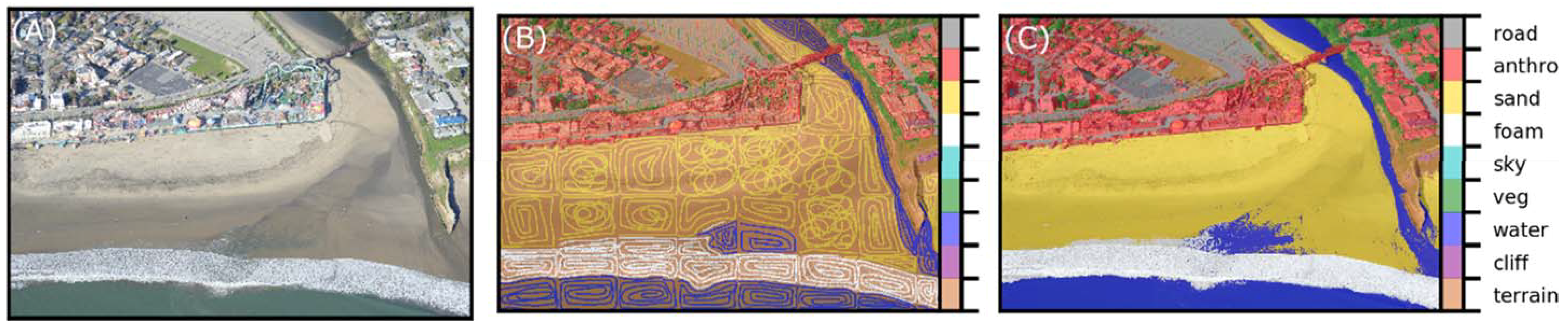
We developed a user-interactive program that segments an image into smaller chunks, the size of which is defined by the user. On each chunk, cycling through a pre-defined set of classes, the user is prompted to draw (using the cursor) example regions of the image that correspond to each label. Unary potentials are derived from these manual on-screen image annotations. These annotations should be exemplative, i.e., a relatively small portion of the region in the chunk that pertains to the class, rather than delimiting the entire region within the chunk that pertains to the class. Typically, the CRF algorithm only requires a few example annotations for each class. For very heterogeneous scenes, however, where each class occurs in several regions across the image (such as the water and anthropogenic classes in Figure 1) example annotations should be provided for each class in each region where that class occurs.
Using this information, the CRF algorithm estimates the class of each pixel in the image (Figure 1). Finally, the image is divided into tiles of a specified size, T. If the proportion of pixels within the tile is greater than a specified amount, Pclass, then the tile is written to a file in a folder denoting its class. This simultaneously and efficiently generates both ground-truth label imagery (to evaluate classification performance) and sets of data suitable for training a DCNN. A single photograph typically takes 5–30 min to process with this method, so all the data required to retrain a DCNN (see section below) may only take up to a few hours to generate. CRF inference time depends primarily on image complexity and size, but is also secondarily affected by the number and spatial heterogeneity of the class labels.
2.3. Retraining a Deep Neural Network (Transfer Learning)
The training library that consists of image tiles, each labeled according to a set of classes, whose generation are described in Section 2.2., is used to retrain an existing DCNN architecture to classify similar unseen image tiles. Among many suitable popular and open-source frameworks for image classification using deep convolutional neural networks, we chose MobileNetV2 [58] because it is relatively small and efficient (computationally faster to train and execute) compared to many competing architectures designed to be transferable for generic image recognition tasks, such as Inception [59], Resnet [60], and NASnet [61], and it is smaller and more accurate than MobileNetV1 [62]. It is also pre-trained for various tile sizes (image windows with horizontal and vertical dimensions of 96, 128, 192, and 224 pixels) which allows us to evaluate that effect on classifications. However, all of the aforementioned models are implemented within TensorFlow-Hub [63], which is a library specifically designed for reusing pre-trained TensorFlow [64] models for new tasks. Like MobileNetV1 [62], MobileNetV2 uses depthwise separable convolutions where, instead of performing a 2D convolution with a kernel, the same result is achieved by doing two 1D convolutions with two kernels, k1 and k2, where k = k1·k2. This requires far fewer parameters, so the model is very small and efficient compared to a model with the same depth using 2D convolution. However, V2 introduces two new features to the architecture: (1) shortcut connections between the bottlenecks called inverted residual layers, and (2) linear bottlenecks between the layers. A bottleneck layer contains few nodes compared to the previous layers, used to obtain a representation of the input with reduced dimensionality [59], leading to large savings in computational cost. Residual layers connect the beginning and end of a convolutional layers with a skip connection, which gives the network access to earlier activations that were not modified in the convolutional layers, and make very deep networks without commensurate increases in parameters. Inverted residuals are a type of residual layer that has fewer parameters, which leads to greater computational efficiency. A “linear” bottleneck is where the last convolution of a residual layer has a linear output before it is added to the initial activations. According to [58], this preserves more information than the more traditional non-linear bottlenecks, which leads to greater accuracy.
For all datasets, we only used tiles (in the training and evaluation) where 90% of the tile pixels were classified as a single class (that is, Pclass > 0.9). This avoided including tiles depicting mixed land cover/use classes. We chose tile sizes of T = 96 × 96 pixels and T = 224 × 224 pixels, which is the full range available for MobileNets, in order to compare the effect of tile size. All model training was carried out in Python using TensorFlow library version 1.7.0. and TensorFlow-Hub version 0.1.0. For each dataset, model training hyperparameters (1000 training epochs, a batch size of 100 images, and a learning rate of 0.01) were kept constant, but not necessarily optimal. For most datasets, there are relatively small numbers of very general classes (water, vegetation, etc.), which, in some ways, creates a more difficult classification task, owing to the greater expected within-class variability associated with broadly-defined categories, than datasets with many more specific classes.
Model retraining (sometimes called “fine-tuning”) consists of tuning the parameters in just the final layer rather than all the weights within all of the network’s layers. Model retraining consists of first using the model, up to the final classifying layer, to generate image feature vectors for each input tile, then retraining only the final, so-called fully-connected model layer that actually does the classification. For each training epoch 100 feature vectors, from tiles chosen at random from the training set, are fed into the final layer to predict the class. Those class predictions are then compared against the actual labels, which is used to update the final layer’s weights through back-propagation.
Each training and testing image tile was normalized against varying illumination and contrast, which greatly aids the transferability of the trained DCNN model. We calculated a normalized image (X′) from a non-normalized image (X) using:
where µ and σ are the mean and standard deviation, respectively [47]. We chose to scale every tile by a maximum possible standard deviation (for an eight-bit image) by using σ = 255. For each tile, µ was chosen as the mean across all three bands for that tile. This procedure could be optimized for a given dataset, but in our study the effects of varying values of σ were minimal.
2.4. CRF-Based Semantic Segmentation
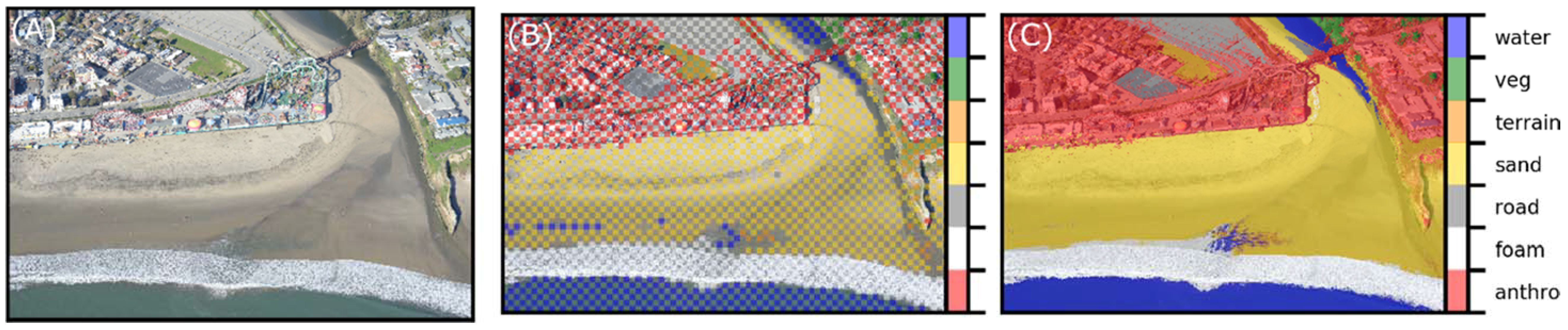
For pixel-scale semantic segmentation of imagery, we have developed a method that harnesses the classification power of the DCNN, with the discriminative capabilities of the CRF. An input image is windowed into small regions of pixels, the size of which is dictated by the size of the tile used in the DCNN training (here, T = 96 × 96 or T = 224 × 224 pixels). Some windows, ideally with an even spatial distribution across the image, are classified with a trained DCNN. Collectively, these predictions serve as unary potentials (known labels) for a CRF to build a probabilistic model for pixelwise classification given the known labels and the underlying image (Figure 2).
Adjustable parameters are: (1) the proportion of the image to estimate unary potentials for (controlled by both T and the number/spacing of tiles), and (2) a threshold probability, Pthres, larger than which a DCNN classification was used in the CRF. Across each dataset, we found that using 50% of the image as unary potentials, and Pthres = 0.5, resulted in good performance. CRF hyperparameters were also held constant across all datasets. We found that good performance across all datasets was achieved using θα = 60, θβ = 5, and θγ = 60. Holding all of these parameters constant facilitates the comparison of the general success of the proposed method. However, it should be noted that accuracy could be further improved for individual datasets by optimizing the parameters for those specific data. This could be achieved by minimizing the discrepancy between ground truth labeled images and model-generated estimates using a validation dataset.
2.5. Metrics to Assess Classification Skill
Standard metrics of precision, P, recall, R, accuracy, A, and F1 score, F, are used to assess classification of image regions and pixels, where TP, TN, FP, and FN are, respectively, the frequencies of true positives, true negatives, false positives, and false negatives:
True positives are image regions/pixels correctly classified as belonging to a certain class by the model, while true negatives are correctly classified as not belonging to a certain class. False negatives are regions/pixels incorrectly classified as not belonging to a certain class, and false positives are those regions/pixels incorrectly classified as belonging to a certain class. Precision and recall are useful where the number of observations belonging to one class is significantly lower than those belonging to the other classes. These metrics are, therefore, used in the evaluation of pixelwise segmentations, where the number of pixels corresponding to each class vary considerably. The F1 score is an equal weighting of the recall and precision and quantifies how well the model performs in general. Recall is a measure of the ability to detect the occurrence of a class, which is a given landform, land use, or land cover.
A “confusion matrix”, which is the matrix of normalized correspondences between true and estimated labels, is a convenient way to visualize model skill. A perfect correspondence between true and estimated labels is scored 1.0 along the diagonal elements of the matrix. Misclassifications are readily identified as off-diagonal elements. Systematic misclassifications are recognized as off-diagonal elements with large magnitudes. Full confusion matrices for each test and dataset are provided in Supplemental 2.
2.6. Data
The chosen datasets encompass a variety of collection platforms (oblique stationary cameras, oblique aircraft, nadir UAV, and nadir satellite) and landforms/land covers, including several shoreline environments (coastal, fluvial, and lacustrine).
2.6.1. NWPU-RESISC45
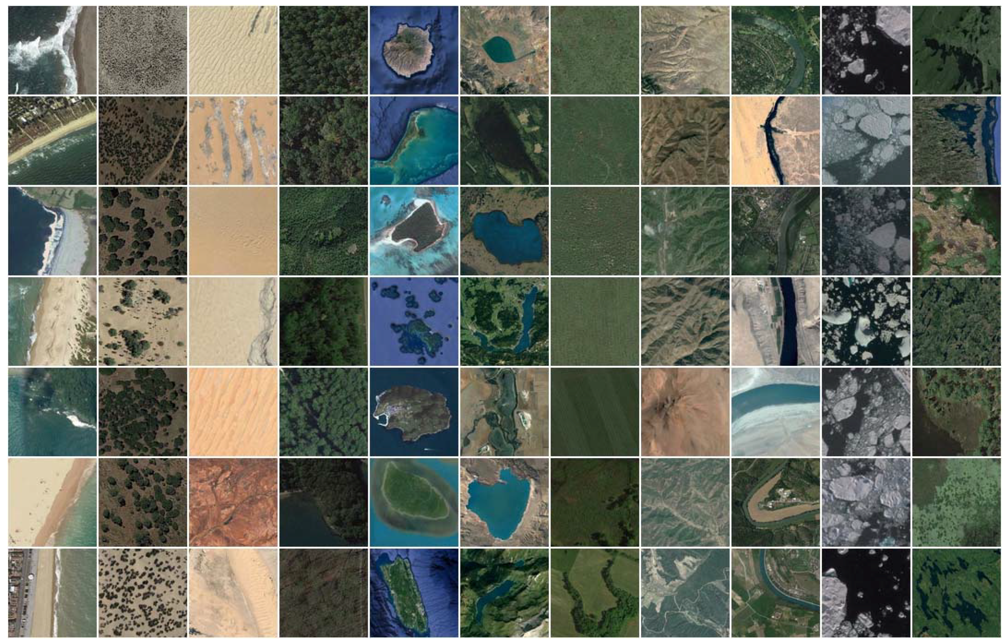
To evaluate the MobileNetV2 DCNN with a conventional satellite-derived land use/land cover dataset, we chose the NWPU-RESISC45, which is a publicly available benchmark for REmote Sensing Image Scene Classification (RESISC), created by Northwestern Polytechnical University (NWPU). The entire dataset, described by [6], contains 31,500 high-resolution images from Google Earth imagery, in 45 scene classes with 700 images in each class. The majority of those classes are urban/anthropogenic. We chose to use a subset of 11 classes corresponding to natural landforms and land cover (Figure 3), namely: beach, chaparral, desert, forest, island, lake, meadow, mountain, river, sea ice, and wetland. All images are 256 × 256 pixels. We randomly chose 350 images from each class for DCNN training, and 350 for testing.
2.6.2. Seabright Beach, CA
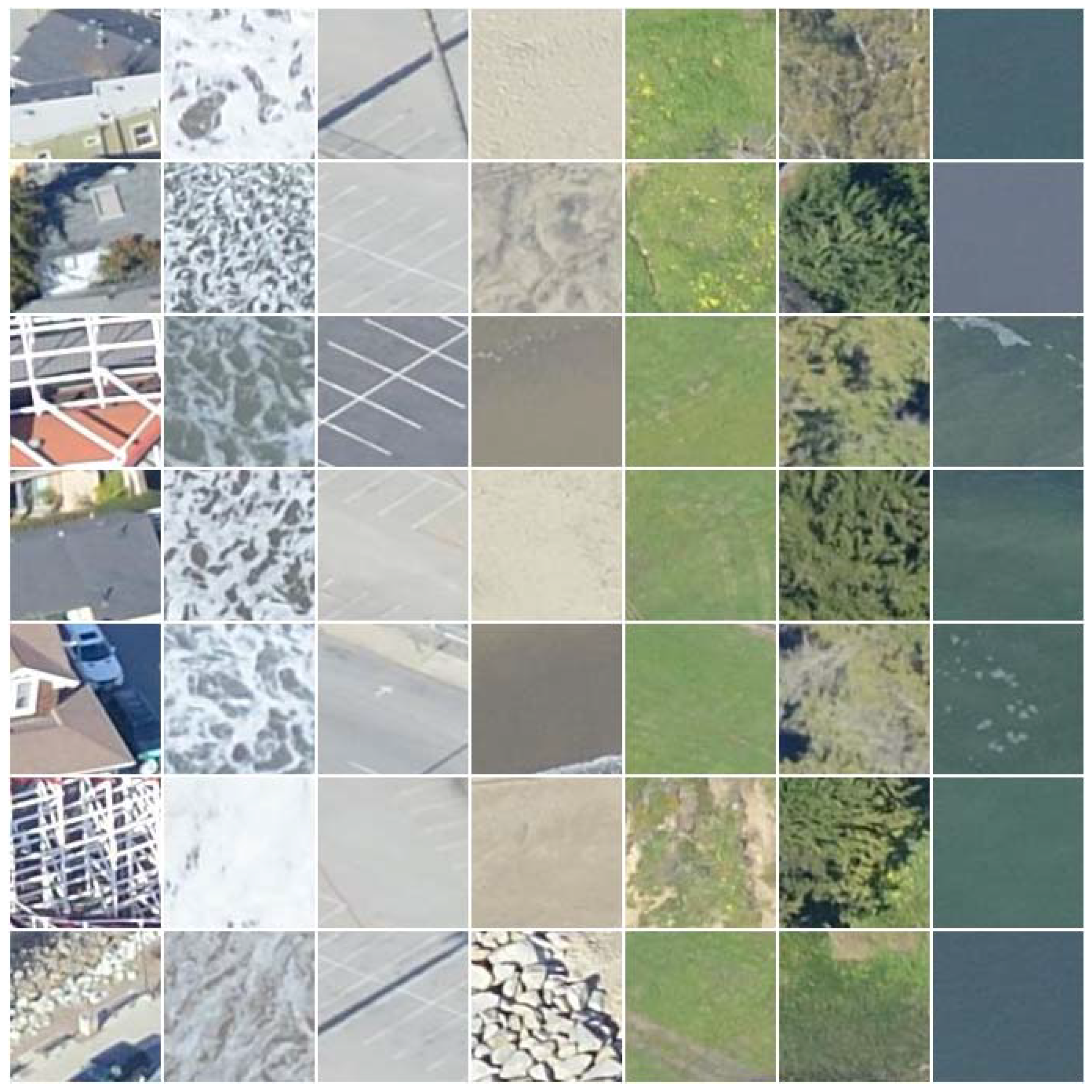
The dataset consists of 13 images of the shorefront at Seabright State Beach, Santa Cruz, CA. Images were collected from a fixed-wing aircraft in February 2016, of which a random subset of seven were used for training, and six for testing (Supplemental 1, Figure S1A,B). Training and testing tiles were generated for seven classes (Table A1 and Figure 2, Figure 3 and Figure 4).
2.6.3. Lake Ontario, NY
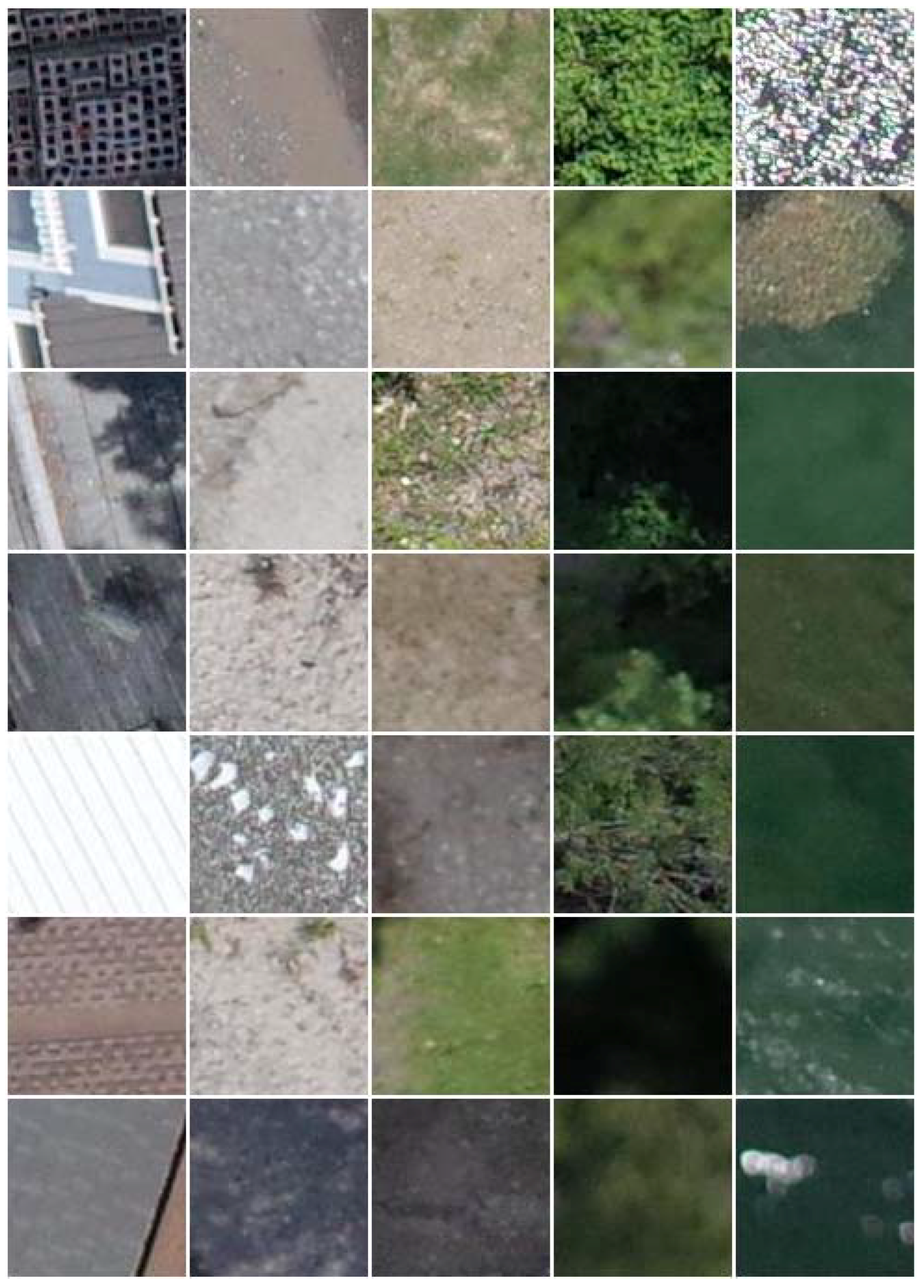
The dataset consists of 48 images obtained in July 2017 from a Ricoh GRII camera mounted to a 3DR Solo quadcopter, a small unmanned aerial system (UAS), flying 80–100 m above ground level in the vicinity of Braddock Bay, New York, on the shores of southern Lake Ontario [65]. A random subset of 24 were used for training, and 24 for testing (Supplemental 1, Figure S1C,D). Training and testing tiles were generated for five classes (Table A2 and Figure 5).
2.6.4. Grand Canyon, AZ
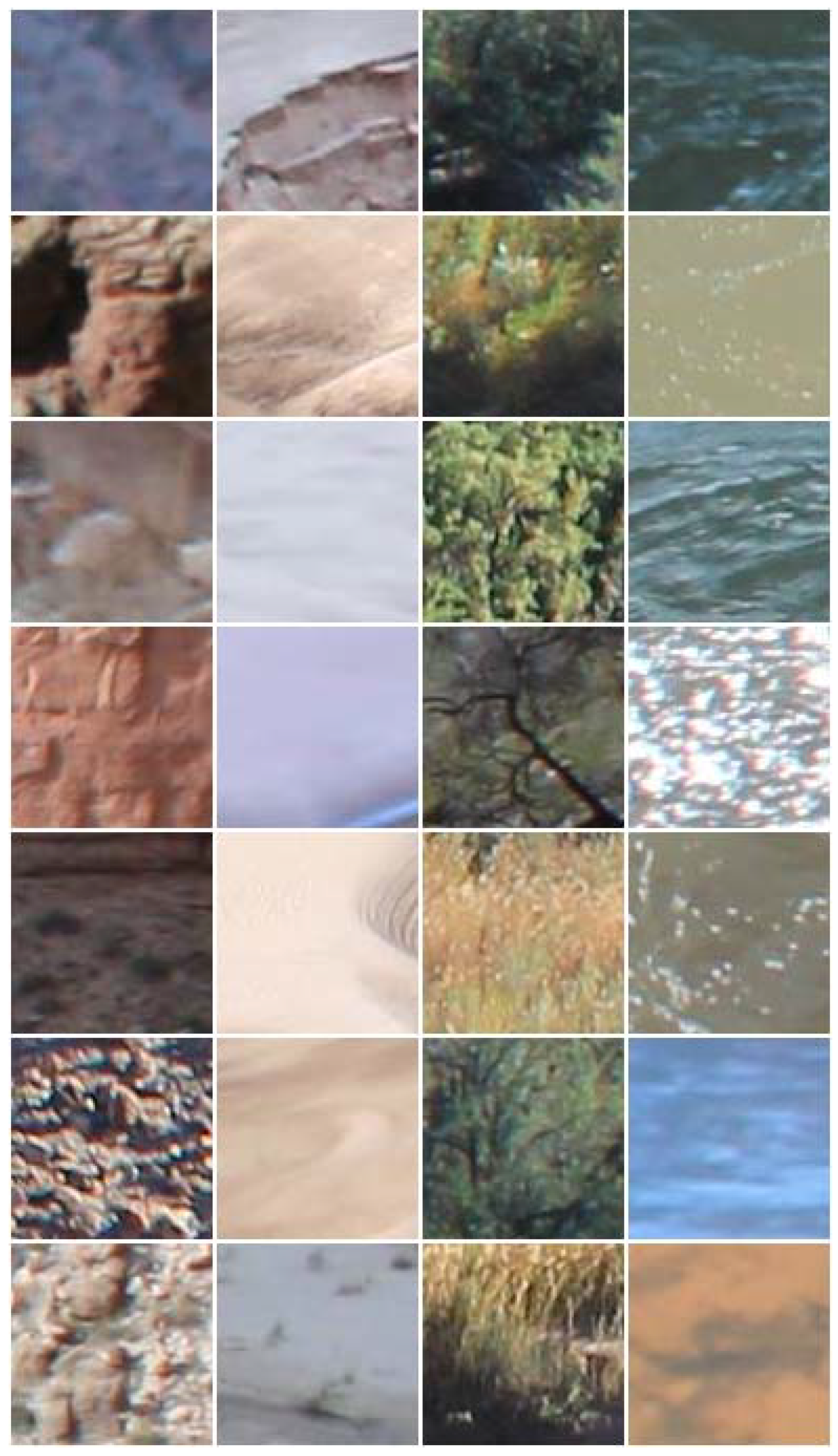
The dataset consists of 14 images collected from a stationary autonomous camera systems monitoring eddy sandbars along the Colorado River in the Grand Canyon. The camera system, sites, and imagery are described in [16]. Imagery came from various seasons and river flow levels, and sites differ considerably in terms of bedrock geology, riparian vegetation, sunlight/shade, and water turbidity. One image from each of seven sites were used for training, and one from each those of the same seven sites were used for testing (Supplemental 1, Figure S1E,F). Training and testing tiles were generated for four classes (Table A3 and Figure 6).
2.6.5. California Coastal Records (CCRP)
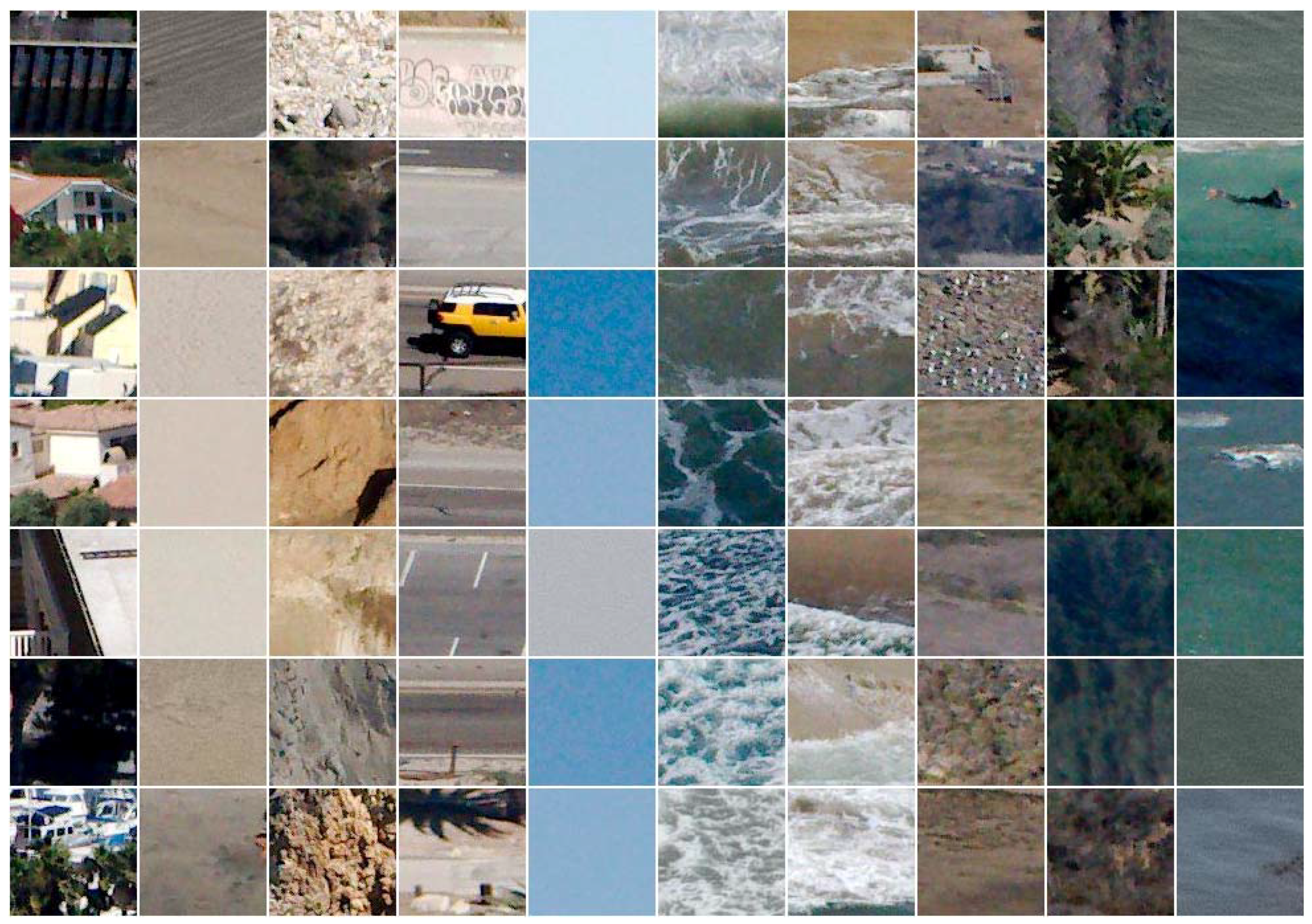
The dataset consists of a sample of 75 images from the California Coastal Records Project (CCRP) [66], of which 45 were used for training, and 30 for testing (Supplemental 1, Figure S1G,H). The photographs were taken over several years and times of the year, from sites all along the California coast, with a handheld digital single-lens reflex camera from a helicopter flying at approximately 50–600 m elevation [20]. The set includes a very wide range of coastal environments, at very oblique angles, with a very large corresponding horizontal footprint. Training and testing tiles were generated for ten classes (Table A4 and Figure 7).
3. Results
3.1. Whole Image Tile Classification Accuracy
For each image set, classes are already available for all image tiles used for testing, so the DCNN model is simply retrained against the pre-defined classes for each dataset. This results in five separate retrained models, one for each of the five datasets. With no fine-tuning of model hyperparameters (of which the most important are the number of training epochs, learning rate, and batch size), we achieved average classification accuracies of between 91% and 98% (F1 scores) across five datasets with T = 224 tiles, and between 88% and 97% with T = 96 tiles (Table 1). Over 26 individual land cover/use classes (Table 2) in four datasets, average classification accuracies ranged between 49% and 99%. Confusion matrices (Supplemental 2, Figure S2A–E) for all classes reveal that most mis-classifications occur between similar groupings, for example, swash and surf, and roads and buildings/anthropogenic. If the model systematically fails to distinguish between certain very similar classes, confusion matrices provide the means with which to identify which classes to group (or, by the same token, split), if necessary, to achieve even greater overall classification accuracies. In most cases, however, the accuracy over all of the classes is less important than the adequate prediction skill for each class, in which case fine-tuning of model hyperparameters should be undertaken to improve differentiation between similar classes. Only for certain data and classes did the distinction between T = 96 and T = 224 tiles make a significant difference, particularly for the Lake Ontario data where classifications were systematically better using T = 224.
3.2. Pixel Classification Accuracy
With no fine-tuning of model hyperparameters, we achieved average pixelwise classification accuracies of between 70% and 78% (F1 scores, Table 3) across four datasets, based on CRF modeling of sparse DCNN predictions with T = 96 tiles (Figure 8). Classification accuracy for a given feature was strongly related to size of that feature (Figure 9). For those land cover/uses that are much greater in size than a 96 × 96 pixels tile, average pixelwise F scores were much higher, ranging from 86% to 90%. Confusion matrices (Supplemental 2, Figure S2F–I) again show how mis-classifications only systematically tend to occur between pairs of the most similar classes. Supplemental 3 shows all semantic segmentations for each image in each dataset.
4. Discussions
Deep learning has revolutionized the field of image classification in recent years [36,37,38,39,42,43,44,45,46,47,48,49]. However, the general usefulness of deep learning applied to conventional photographic imagery at the landscape scale is, at yet, largely unproven. Here, consistent with previous studies that have demonstrated the ability of DCNNs for classification of land use/cover in long-range remotely-sensed imagery from satellites [6,9,45,46,47,48,49], we demonstrated that DCNNs are powerful tools for classifying landforms and land cover in medium-range imagery acquired from UAS, aerial, and ground-based platforms. Further, we found that the smallest and most computationally efficient widely available DCNN architecture, MobilenetsV2, classifies land use/cover with comparable accuracies to larger, slower, DCNN models, such as AlexNet [6,45,67], VGGNet [6,45,68], GoogLeNet [6,69,70], or custom-designed DCNNs [9,46,47]. Although we deliberately chose a standard set of model parameters, and achieved reasonable pixel-scale classifications across all classes, even greater accuracy is likely attainable with a model fine-tuned to a particular dataset [6]. Here, reported pixel-scale classification accuracies are only estimates because they do not take into account potential errors in the ground truth data (label images) which could have arisen due to human error and/or imperfect CRF pixel classification. A more rigorous quantification of classification accuracy would require painstaking pixel-level classification of imagery using a fully manual approach, which would take hours to days for each image, possibly in conjunction with field measurements, to verify land cover represented in imagery.
In remote sensing, the acquisition of pixel-level reference/label data is time-consuming and limiting [46], so acquiring a suitably large dataset for training the DCNN is often a significant challenge. Therefore, most studies that use pixel-level classifications only use a few hundred reference points [71,72]. We suggest a new method for generating pixel-level labeled imagery for use in developing and evaluating classifications (DCNN-based and others), based on manual on-screen annotations in combination with a fully-connected conditional random field (CRF, Figure 1). As stated in Section 2.2, the CRF model will typically only require a few example annotations for each class as priors, so for efficiency’s sake annotations should be more exemplative than exhaustive, i.e., relatively small portions of the regions of the image associated with each class. However, the optimal number and extent of annotations depends on the scene and the (number of) classes and, therefore, learning an optimal annotating process for a given set of images is highly experiential.
This method for generating label imagery will find general utility for training and testing any algorithm for pixelwise image classification. We show that in conjunction with transfer learning and small, efficient DCNNs, it provides the means to rapidly train a DCNN with a small dataset. In turn, this facilitates the rapid assessment of the general utility of DCNN architectures for a given classification problem, and provides the means to fine-tune a feature class or classes iteratively based on classification mismatches. The workflow presented here can be used to quickly assess the potential of a small DCNN like MobilenetV2 for a specific classification task. This ‘prototyping’ stage can also be used to assess classes that should be grouped, or split, depending on the analysis of the confusion matrices, such as presented in Supplemental 2, Figure S2A–E. If promising, larger models, such as Resnet [60] or NASnet [61] could be used, within the same framework provided by Tensorflow Hub, for even greater classification accuracy.
Recognizing the capabilities of the CRF as a discriminative classification algorithm given a set of sparse labels, we propose a pixel-wise semantic segmentation algorithm based upon DCNN-estimated regions of images in combination with the fully-connected CRF. We offer this hybrid DCNN-CRF approach to semantic segmentation as a simpler alternative to so-called `fully convolutional’ DCNNs [8,39,73] which, in order to achieve accurate pixel level classifications, require much larger, more sophisticated DCNN architectures [37], which are often computationally more demanding to train. Since pooling within the DCNN results in a significant loss of spatial resolution, these architectures require an additional set of convolutional layers that learn the ‘upscaling’ between the last pooling layer, which will be significantly smaller than the input image, and the pixelwise labelling at the required finer resolution. This process is imperfect, therefore, label images appear coarse at the object/label boundaries [73] and some post-processing algorithms, such as a CRF or similar approach, is required to refine the predictions. Due to this, we also suggest that our hybrid approach might be a simpler approach to semantic segmentation, especially for rapid prototyping (as discussed above) and in the cases where the scales of spatially continuous features are larger than the tile size used in the DCNN (Figure 9). However, for spatially isolated features, especially those that exist throughout small spatially contiguous areas, the more complicated fully-convolutional approach to pixelwise classification might be necessary.
The CRF is designed to classify (or in some instances, where some unary potentials are considered improbable by the CRF model, reclassify) pixels based on both the color/brightness and the proximity of nearby pixels with the same label. When DCNN predictions are used as unary potentials, we found that, typically, the CRF algorithm requires them, ideally regularly spaced, for approximately one quarter of the pixels in relatively simple scenes, and about one half in relatively complicated scenes (e.g., Figure 10B) for satisfactory pixelwise classifications (e.g., Figure 10C). With standardized parameter values that were not fine-tuned to individual images or datasets, CRF performance was mixed, especially for relatively small objects/features (Table 3). This is exemplified by Figure 10, where several small outcropping rocks, whose pixel labels were not included as CRF unary potentials, were either correctly or incorrectly labeled by the CRF, despite the similarity in their location, size, color, and their relative proximity to correctly-labeled unary potentials. Dark shadows on cliffs were sometimes misclassified as water, most likely because the water class contains examples of shallow kelp beds, which are also almost black. A separate “shadow” or “kelp” class might have ameliorated this issue. We found that optimizing CRF parameters to reduce such misclassifications could be done for an individual image, but not in a systematic way that would improve similar misclassifications in other images. Whereas here we have used RGB imagery, the CRF would work in much the same way with larger multivariate datasets, such as multispectral or hyperspectral imagery, or other raster stacks consisting of information on coincident spatial grids.
If DCNN-based image classification is to gain wider application and acceptance within the geoscience community, similar demonstrable examples, need to be coupled with accessible tools and datasets to develop deep neural network architectures that better discriminate landforms and land uses in landscape imagery. To that end, we invite interested readers to use our data and code (see Acknowledgements) to explore variations in classifications among multiple DCNN architectures, and to use our extensive pixel-level label dataset to evaluate and facilitate the development of custom DCNN models for specific classification tasks in the geosciences.
5. Conclusions
In summary, we have developed a workflow for efficiently creating labeled imagery, retraining DCNNs for image recognition, and semantic classification of imagery. A user-interactive tool has been developed that enables the manual delineation of exemplative regions in the input image of specific classes in conjunction with a fully-connected conditional random field (CRF) to estimate the class for every pixel within the image. The resulting label imagery can be used to train and test DCNN models. Training and evaluation datasets are created by selecting tiles from the image that contains a proportion of pixels that correspond to a given class that is greater than a given threshold. The training tiles are then used to retrain a DCNN. We chose the MobileNetsV2 framework, but any one of several similar models may alternatively be used. The retrained DCNN is used to classify small spatially-distributed regions of pixels in a sample image, which is used in conjunction with the same CRF method used for label image creation to estimate a class for every pixel in the image.
Our work demonstrates the general effectiveness of a repurposed, small, very fast, existing DCNN framework (MobileNetV2) for classification of landforms, land use, and land cover features in both satellite and high-vantage, oblique, and nadir imagery collected using planes, UAVs, and static monitoring cameras. With no fine tuning of model parameters, we achieve average classification accuracies of between 91% and 98% (F1 scores) across five disparate datasets, ranging between 71% and 99% accuracies over 26 individual land cover/use classes across four datasets. Further, we demonstrate how structured prediction using a fully-connected CRF can be used in a semi-supervised manner to very efficiently generate ground truth label imagery and DCNN training libraries. Finally, we propose a hybrid method for accurate semantic segmentation of imagery of natural landscapes based on combining (1) the recognition capacity of DCNNs to classify small regions in imagery, and (2) the fine grained localization of fully-connected CRFs for pixel-level classification. Where land cover/uses that are typically much greater in size than a 96 × 96 pixel tile, average pixelwise F1 scores range from 86% to 90%. Smaller, and more isolated features have greater pixelwise accuracies. This is in part due to our usage of a common set of model parameters for all datasets, however, further refinement of this technique may be required to classify features that are much smaller than a 96 × 96 pixel tile with similar accuracies as larger features and land covers.
These techniques should find numerous application in the classification of remotely-sensed imagery for geomorphic and natural hazard studies, especially for rapidly evaluating the general utility of DCNNs for a specific classification task, and especially for relatively large and spatially extensive land cover types. All of our data, trained models, and processing scripts are available at https://github.com/dbuscombe-usgs/dl_landscapes_paper.
Supplementary Materials
The following are available online at https://www.mdpi.com/2076-3263/8/7/244/s1, Supplemental 1: Datasets, Supplemental 2: Confusion matrices, Supplemental 3: DCNN-CRF classifications.
Author Contributions
Conceptualization: D.B. and A.C.R.; methodology: D.B. and A.C.R.; software: D.B.; validation: D.B.; formal analysis: D.B.; data curation: D.B.; writing—original draft preparation: D.B. and A.C.R.; writing—review and editing: D.B. and A.C.R.; visualization: D.B.; and funding acquisition: D.B.
Funding
This research was funded by the U.S. Geological Survey Pacific Coastal and Marine Geology and Grand Canyon Monitoring and the Research Center, by means of two awards to Northern Arizona University (USGS Agreements G17AS00003 and G16AC00280).
Acknowledgments
Thanks to Jon Warrick, Paul Grams, and Chris Sherwood for data and discussions. Images from the California Coastal Records Project are Copyright (C) 2002–2018 Kenneth and Gabrielle Adelman, www.Californiacoastline.org and are used with permission. Any use of trade, firm, or product names is for descriptive purposes only and does not imply endorsement by the U.S. Government. All of our data, trained models, and processing scripts are available at https://github.com/dbuscombe-usgs/dl_landscapes_paper.
Conflicts of Interest
The authors declare no conflict of interest.
Appendix A

Table A1.
Classes and number of tiles used for the Seabright dataset.
| Class | Number of Training Tiles (T = 96/224) | Number of Evaluation Tiles (T = 96/224) |
|---|---|---|
| Anthropogenic/buildings | 23,566/4548 | 15,575/3031 |
| Road/pavement | 314/60 | 525/103 |
| Sand | 38,250/6887 | 25,318/5802 |
| Vegetation | 386/76 | 240/38 |
| Other terrain | 77/24 | 117/22 |
| Water | 11,394/1723 | 14,360/2251 |
| Foam | 5076/735 | 5139/843 |
| Total: | 76,063/14,053 | 61,274/12,090 |
Table A2.
Classes and number of tiles used for the Lake Ontario dataset.
| Class | Number of Training Tiles (T = 96/224) | Number of Evaluation Tiles (T = 96/224) |
|---|---|---|
| Anthropogenic/buildings | 467/219 | 3216/333 |
| Sediment | 2856/289 | 3758/407 |
| Vegetation | 33,871/5139 | 33,421/5001 |
| Other terrain | 1596/157 | 1094/92 |
| Water | 80,304/13,332 | 77,571/12,950 |
| Total: | 119,094/19,136 | 119,060/18,783 |
Table A3.
Classes and number of tiles used for the Grand Canyon dataset.
| Class | Number of Training Tiles (T = 96/224) | Number of Evaluation Tiles (T = 96/224) |
|---|---|---|
| Rock/scree/terrain | 15,059/2405 | 12,151/1999 |
| Sand | 751/39 | 1069/91 |
| Riparian vegetation | 2971/408 | 2158/305 |
| Water | 8568/1462 | 5277/1130 |
| Total: | 27,349/4314 | 20,655/3525 |
Table A4.
Classes and number of tiles used for the California Coastal Records dataset.
| Class | Number of Training Tiles (T = 96/224) | Number of Evaluation Tiles (T = 96/224) |
|---|---|---|
| Beach | 39,206/6460 | 42,616/7438 |
| Anthropogenic/buildings | 34,585/6904 | 45,831/8452 |
| Cliff | 29,844/4666 | 17,488/3108 |
| Road | 6000/705 | 3782/440 |
| Sky | 41,139/6694 | 26,240/4267 |
| Surf/foam | 18,775/2745 | 25,025/3549 |
| Swash | 5825/1280 | 4535/552 |
| Other terrain | 87,632/18,517 | 50,254/8647 |
| Vegetation | 81,896/19,346 | 46,097/7639 |
| Water | 121,684/17,123 | 49,427/11,019 |
| Total: | 466,586/84,440 | 311,295/55,111 |
References
- Franklin, S.E.; Wulder, M.A. Remote sensing methods in medium spatial resolution satellite data land cover classification of large areas. Prog. Phys. Geogr. 2002, 26, 173–205. [Google Scholar] [CrossRef]
- Smith, M.J.; Pain, C.F. Applications of remote sensing in geomorphology. Prog. Phys. Geogr. 2009, 33, 568–582. [Google Scholar] [CrossRef]
- Mulder, V.L.; De Bruin, S.; Schaepman, M.E.; Mayr, T.R. The use of remote sensing in soil and terrain mapping—A review. Geoderma 2011, 162, 1–19. [Google Scholar] [CrossRef]
- Sekovski, I.; Stecchi, F.; Mancini, F.; Del Rio, L. Image classification methods applied to shoreline extraction on very high-resolution multispectral imagery. Int. J. Remote Sens. 2014, 35, 3556–3578. [Google Scholar] [CrossRef]
- Ma, L.; Li, M.; Ma, X.; Cheng, L.; Du, P.; Liu, Y. A review of supervised object-based land-cover image classification. ISPRS J. Photogramm. 2017, 130, 277–293. [Google Scholar] [CrossRef]
- Cheng, G.; Han, J.; Lu, X. Remote sensing image scene classification: Benchmark and state of the art. Proc. IEEE 2017, 105, 1865–1883. [Google Scholar] [CrossRef]
- O’Connor, J.; Smith, M.J.; James, M.R. Cameras and settings for aerial surveys in the geosciences: Optimising image data. Prog. Phys. Geogr. 2017, 41, 325–344. [Google Scholar] [CrossRef]
- Long, J.; Shelhamer, E.; Darrell, T. Fully convolutional networks for semantic segmentation. In Proceedings of the 2015 IEEE Conference on Computer Vision and Pattern Recognition (CVPR), Boston, MA, USA, 7–12 June 2015; pp. 3431–3440. [Google Scholar]
- Volpi, M.; Tuia, D. Dense semantic labeling of subdecimeter resolution images with convolutional neural networks. IEEE Trans. Geosci. Remote 2017, 55, 881–893. [Google Scholar] [CrossRef]
- Holman, R.A.; Stanley, J. The history and technical capabilities of Argus. Coast. Eng. 2007, 54, 477–491. [Google Scholar] [CrossRef]
- Bertoldi, W.; Zanoni, L.; Tubino, M. Assessment of morphological changes induced by flow and flood pulses in a gravel bed braided river: The Tagliamento River (Italy). Geomorphology 2010, 114, 348–360. [Google Scholar] [CrossRef]
- Hoonhout, B.; Radermacher, M.; Baart, F.; Van der Maaten, L. An automated method for semantic classification of regions in coastal images. Coast. Eng. 2015, 105, 1–12. [Google Scholar] [CrossRef] [Green Version]
- Bergsma, E.; Conley, D.; Davidson, M.; O’Hare, T. Video-based nearshore bathymetry estimation in macro-tidal environments. Mar. Geol. 2016, 374, 31–41. [Google Scholar] [CrossRef]
- Almar, R.; Larnier, S.; Castelle, B.; Scott, T. On the use of the radon transform to estimate longshore currents from video imagery. Coast. Eng. 2016, 114, 301–308. [Google Scholar] [CrossRef]
- Benacchio, V.; Piégay, H.; Buffin-Bélanger, T.; Vaudor, L. A new methodology for monitoring wood fluxes in rivers using a ground camera: Potential and limits. Geomorphology 2017, 279, 44–58. [Google Scholar] [CrossRef]
- Grams, P.E.; Tusso, R.B.; Buscombe, D. Automated Remote Cameras for Monitoring Alluvial Sandbars on the Colorado River in Grand Canyon, Arizona; USGS Open File Report, No. 2018-1019; US Geological Survey: Reston, VA, USA, 2018.
- Turner, I.L.; Harley, M.D.; Drummond, C.D. UAVs for coastal surveying. Coast. Eng. 2016, 114, 19–24. [Google Scholar] [CrossRef]
- Su, L.; Gibeaut, J. Using UAS hyperspatial RGB imagery for identifying beach zones along the south Texas coast. Remote Sens. 2017, 9, 159. [Google Scholar] [CrossRef]
- Sturdivant, E.J.; Lentz, E.E.; Thieler, E.R.; Farris, A.S.; Weber, K.M.; Remsen, D.P.; Miner, S.; Henderson, R.E. UAS-SfM for Coastal Research: Geomorphic Feature Extraction and Land Cover Classification from High-Resolution Elevation and Optical Imagery. Remote Sens. 2017, 9, 1020. [Google Scholar] [CrossRef]
- Warrick, J.A.; Ritchie, A.C.; Adelman, G.; Adelman, K.; Limber, P.W. New techniques to measure cliff change from historical oblique aerial photographs and structure-from-motion photogrammetry. J. Coast. Res. 2016, 33, 39–55. [Google Scholar] [CrossRef]
- Fonstad, M.A.; Dietrich, J.T.; Courville, B.C.; Jensen, J.L.; Carbonneau, P.E. Topographic structure from motion: A new development in photogrammetric measurement. Earth Surf. Proc. Land. 2013, 38, 421–430. [Google Scholar] [CrossRef]
- Javernick, L.; Brasington, J.; Caruso, B. Modeling the topography of shallow braided rivers using Structure-from-Motion photogrammetry. Geomorphology 2014, 213, 166–182. [Google Scholar] [CrossRef]
- Woodget, A.S.; Austrums, R. Subaerial gravel size measurement using topographic data derived from a UAV-SfM approach. Earth Surf. Proc. Land. 2017, 42, 1434–1443. [Google Scholar] [CrossRef] [Green Version]
- Carbonneau, P.E.; Bizzi, S.; Marchetti, G. Robotic photosieving from low-cost multirotor sUAS: A proof-of-concept. Earth Surf. Proc. Land. 2018. [Google Scholar] [CrossRef]
- Hugenholtz, C.H.; Whitehead, K.; Brown, O.W.; Barchyn, T.E.; Moorman, B.J.; LeClair, A.; Riddell, K.; Hamilton, T. Geomorphological mapping with a small unmanned aircraft system (sUAS): Feature detection and accuracy assessment of a photogrammetrically-derived digital terrain model. Geomorphology 2013, 194, 16–24. [Google Scholar] [CrossRef] [Green Version]
- Pajares, G. Overview and current status of remote sensing applications based on unmanned aerial vehicles (UAVs). Photogramm. Eng. Remote Sens. 2015, 81, 281–329. [Google Scholar] [CrossRef]
- Xie, Y.; Sha, Z.; Yu, M. Remote sensing imagery in vegetation mapping: A review. J. Plant Ecol. 2008, 1, 9–23. [Google Scholar] [CrossRef]
- Adam, E.; Mutanga, O.; Rugege, D. Multispectral and hyperspectral remote sensing for identification and mapping of wetland vegetation: A review. Wetl. Ecol. Manag. 2010, 18, 281–296. [Google Scholar] [CrossRef]
- Dugdale, S.J.; Bergeron, N.E.; St-Hilaire, A. Spatial distribution of thermal refuges analysed in relation to riverscape hydromorphology using airborne thermal infrared imagery. Remote Sens. Environ. 2015, 160, 43–55. [Google Scholar] [CrossRef]
- Tamminga, A.; Hugenholtz, C.; Eaton, B.; Lapointe, M. Hyperspatial remote sensing of channel reach morphology and hydraulic fish habitat using an unmanned aerial vehicle (UAV): A first assessment in the context of river research and management. River Res. Appl. 2015, 31, 379–391. [Google Scholar] [CrossRef]
- Bryant, R.G.; Gilvear, D.J. Quantifying geomorphic and riparian land cover changes either side of a large flood event using airborne remote sensing: River Tay, Scotland. Geomorphology 1999, 29, 307–321. [Google Scholar] [CrossRef]
- East, A.E.; Pess, G.R.; Bountry, J.A.; Magirl, C.S.; Ritchie, A.C.; Logan, J.B.; Randle, T.J.; Mastin, M.C.; Minear, J.T.; Duda, J.J.; et al. Large-scale dam removal on the Elwha River, Washington, USA: River channel and floodplain geomorphic change. Geomorphology 2015, 228, 765–786. [Google Scholar] [CrossRef]
- Warrick, J.A.; Bountry, J.A.; East, A.E.; Magirl, C.S.; Randle, T.J.; Gelfenbaum, G.; Ritchie, A.C.; Pess, G.R.; Leung, V.; Duda, J.J. Large-scale dam removal on the Elwha River, Washington, USA: Source-to-sink sediment budget and synthesis. Geomorphology 2015, 246, 729–750. [Google Scholar] [CrossRef]
- LeCun, Y.; Bengio, Y.; Hinton, G. Deep learning. Nature 2015, 521, 436. [Google Scholar] [CrossRef] [PubMed]
- Goodfellow, I.; Bengio, Y.; Courville, A.; Bengio, Y. Deep Learning; MIT Press: Cambridge, UK, 2016; Volume 1. [Google Scholar]
- Szegedy, C.; Ioffe, S.; Vanhoucke, V.; Alemi, A.A. Inception-v4, Inception-Resnet and the impact of residual connections on learning. In Proceedings of the Thirty-First AAAI Conference on Artificial Intelligence, San Francisco, CA, USA, 4–9 February 2017; Volume 4, p. 12. [Google Scholar]
- Chen, L.C.; Papandreou, G.; Kokkinos, I.; Murphy, K.; Yuille, A.L. Deeplab: Semantic image segmentation with deep convolutional nets, atrous convolution, and fully connected crfs. IEEE Trans. Pattern Anal. Mach. Intell. 2018, 40, 834–848. [Google Scholar] [CrossRef] [PubMed]
- Litjens, G.; Kooi, T.; Bejnordi, B.E.; Setio, A.A.A.; Ciompi, F.; Ghafoorian, M.; van der Laak, J.A.; van Ginneken, B.; Sánchez, C.I. A survey on deep learning in medical image analysis. Med. Image Anal. 2017, 42, 60–88. [Google Scholar] [CrossRef] [PubMed] [Green Version]
- Maggiori, E.; Tarabalka, Y.; Charpiat, G.; Alliez, P. Convolutional neural networks for large-scale remote-sensing image classification. IEEE Trans. Geosci. Remote Sens. 2017, 55, 645–657. [Google Scholar] [CrossRef]
- Belgiu, M.; Drăguţ, L. Random forest in remote sensing: A review of applications and future directions. ISPRS J. Photogramm. 2016, 114, 24–31. [Google Scholar] [CrossRef]
- Dauphin, Y.N.; Pascanu, R.; Gulcehre, C.; Cho, K.; Ganguli, S.; Bengio, Y. Identifying and attacking the saddle point problem in high-dimensional non-convex optimization. In Advances in Neural Information Processing Systems; MIT Press: Cambridge, MA, USA, 2014; pp. 2933–2941. [Google Scholar]
- Garcia-Garcia, A.; Orts-Escolano, S.; Oprea, S.; Villena-Martinez, V.; Garcia-Rodriguez, J. A review on deep learning techniques applied to semantic segmentation. arXiv, 2017; arXiv:1704.06857. [Google Scholar]
- Deng, J.; Dong, W.; Socher, R.; Li, L.J.; Li, K.; Fei-Fei, L. Imagenet: A large-scale hierarchical image database. In Proceedings of the 2009 IEEE Conference on Computer Vision and Pattern Recognition, Miami, FL, USA, 20–25 June 2009; pp. 248–255. [Google Scholar]
- Russakovsky, O.; Deng, J.; Su, H.; Krause, J.; Satheesh, S.; Ma, S.; Huang, Z.; Karpathy, A.; Khosla, A.; Bernstein, M.; et al. ImageNet Large Scale Visual Recognition Challenge. Int. J. Comput. Vis. 2015, 115, 211–252. [Google Scholar] [CrossRef] [Green Version]
- Hu, F.; Xia, G.S.; Hu, J.; Zhang, L. Transferring deep convolutional neural networks for the scene classification of high-resolution remote sensing imagery. Remote Sens. 2015, 7, 14680–14707. [Google Scholar] [CrossRef]
- Längkvist, M.; Kiselev, A.; Alirezaie, M.; Loutfi, A. Classification and Segmentation of Satellite Orthoimagery Using Convolutional Neural Networks. Remote Sens. 2016, 8, 329. [Google Scholar] [CrossRef]
- Palafox, L.F.; Hamilton, C.W.; Scheidt, S.P.; Alvarez, A.M. Automated detection of geological landforms on Mars using Convolutional Neural Networks. Comput. Geosci. 2017, 101, 48–56. [Google Scholar] [CrossRef] [PubMed]
- Lu, H.; Fu, X.; Liu, C.; Li, L.G.; He, Y.X.; Li, N.W. Cultivated land information extraction in UAV imagery based on deep convolutional neural network and transfer learning. J. Mt. Sci. 2017, 14, 731–741. [Google Scholar] [CrossRef]
- Marmanis, D.; Datcu, M.; Esch, T.; Stilla, U. Deep Learning Earth Observation Classification Using ImageNet Pretrained Networks. IEEE Geosci. Remote Sens. Lett. 2016, 13, 105–109. [Google Scholar] [CrossRef]
- Sutton, C.; McCallum, A. Introduction to statistical relational learning. In An Introduction to Conditional Random Fields for Relational Learning; MIT Press: Cambridge, MA, USA, 2006; Volume 2. [Google Scholar]
- Koller, D.; Friedman, N. Probabilistic Graphical Models: Principles and Techniques; MIT Press: Cambridge, MA, USA, 2009. [Google Scholar]
- Lafferty, J.; McCallum, A.; Pereira, F. Conditional random fields: Probabilistic models for segmenting and labeling sequence data. In Proceedings of the 18th International Conference on Machine Learning, Williamstown, MA, USA, 28 June–1 July 2001; p. 282. [Google Scholar]
- Kumar, S.; Hebert, M. Discriminative random fields. Int. J. Comput. Vis. 2006, 68, 179–201. [Google Scholar] [CrossRef]
- Tappen, M.; Liu, C.; Adelson, E.; Freeman, W. Learning Gaussian conditional random fields for low-level vision. In Proceedings of the 2007 IEEE Conference on Computer Vision and Pattern Recognition, Minneapolis, MN, USA, 17–22 June 2007; pp. 1–8. [Google Scholar]
- Krahenbuhl, P.; Koltun, V. Efficient inference in fully connected CRFs with Gaussian edge potentials. Adv. Neural Inf. Process. Syst. 2011, 24, 109–117. [Google Scholar]
- Zhu, H.; Meng, F.; Cai, J.; Lu, S. Beyond pixels: A comprehensive survey from bottom-up to semantic image segmentation and cosegmentation. J. Vis. Commun. Image Represent. 2016, 34, 12–27. [Google Scholar] [CrossRef] [Green Version]
- Chen, L.C.; Yang, Y.; Wang, J.; Xu, W.; Yuille, A.L. Attention to scale: Scale-aware semantic image segmentation. In Proceedings of the 2016 IEEE Conference on Computer Vision and Pattern Recognition, Las Vegas, NV, USA, 26 June–1 July 2016; pp. 3640–3649. [Google Scholar]
- Sandler, M.; Howard, A.; Zhu, M.; Zhmoginov, A.; Chen, L.C. Inverted Residuals and Linear Bottlenecks: Mobile Networks for Classification, Detection and Segmentation. arXiv, 2018; arXiv:1801.04381. [Google Scholar]
- Szegedy, C.; Vanhoucke, V.; Ioffe, S.; Shlens, J.; Wojna, Z. Rethinking the inception architecture for computer vision. In Proceedings of the 2016 IEEE Conference on Computer Vision and Pattern Recognition, Las Vegas, NV, USA, 26 June–1 July 2016; pp. 2818–2826. [Google Scholar]
- He, K.; Zhang, X.; Ren, S.; Sun, J. Deep residual learning for image recognition. In Proceedings of the 2016 IEEE Conference on Computer Vision and Pattern Recognition, Las Vegas, NV, USA, 26 June–1 July 2016; pp. 770–778. [Google Scholar]
- Zoph, B.; Vasudevan, V.; Shlens, J.; Le, Q.V. Learning transferable architectures for scalable image recognition. arXiv, 2017; arXiv:1707.07012. [Google Scholar]
- Howard, A.G.; Zhu, M.; Chen, B.; Kalenichenko, D.; Wang, W.; Weyand, T.; Andreetto, M.; Adam, H. Mobilenets: Efficient convolutional neural networks for mobile vision applications. arXiv, 2017; arXiv:1704.04861. [Google Scholar]
- TensorFlow-Hub 2018. Available online: https://www.tensorflow.org/hub/modules/image (accessed on 1 June 2018).
- Abadi, M.; Agarwal, A.; Barham, P.; Brevdo, E.; Chen, Z.; Citro, C.; Corrado, G.S.; Davis, A.; Dean, J.; Devin, M.; et al. TensorFlow: Large-Scale Machine Learning on Heterogeneous Systems. 2015. Available online: https://www.tensorflow.org (accessed on 1 June 2018).
- Sherwood, C.R.; Brosnahan, S.M.; Ackerman, S.D.; Borden, J.; Montgomery, E.T.; Pendleton, E.A.; Sturdivant, E.J. Aerial Imagery and Photogrammetric Products from Unmanned Aerial Systems (UAS) Flights over the Lake Ontario Shoreline at Braddock Bay, New York, July 10 to 11, 2017. 2018. Available online: https://doi.org/10.5066/F74F1PX3 (accessed on 1 June 2018).
- California Coastal Records Project (CCRP). 2018. Available online: http://www.californiacoastline.org/ (accessed on 1 June 2018).
- Krizhevsky, A.; Sutskever, I.; Hinton, G.E. Imagenet classification with deep convolutional neural networks. In Advances in Neural Information Processing Systems; Curran Associates Inc.: New York, NY, USA, 2012; pp. 1097–1105. [Google Scholar]
- Simonyan, K.; Zisserman, A. Very deep convolutional networks for large-scale image recognition. arXiv, 2014; arXiv:1409.1556. [Google Scholar]
- Szegedy, C.; Liu, W.; Jia, Y.; Sermanet, P.; Reed, S.; Anguelov, D.; Erhan, D.; Vanhoucke, V.; Rabinovich, A. Going deeper with convolutions. In Proceedings of the 2015 IEEE Conference on Computer Vision and Pattern Recognition (CVPR), Boston, MA, USA, 7–12 June 2015; pp. 1–9. [Google Scholar]
- Castelluccio, M.; Poggi, G.; Sansone, C.; Verdoliva, L. Land use classification in remote sensing images by convolutional neural networks. arXiv, 2015; arXiv:1508.00092. [Google Scholar]
- Li, X.; Shao, G. Object-based land-cover mapping with high resolution aerial photography at a county scale in midwestern USA. Remote Sens. 2014, 6, 11372–11390. [Google Scholar] [CrossRef]
- Thomas, N.; Hendrix, C.; Congalton, R.G. A comparison of urban mapping methods using high-resolution digital imagery. Photogramm. Eng. Remote Sens. 2003, 69, 963–972. [Google Scholar] [CrossRef]
- Fu, G.; Liu, C.; Zhou, R.; Sun, T.; Zhang, Q. Classification for high resolution remote sensing imagery using a fully convolutional network. Remote Sens. 2017, 9, 498. [Google Scholar] [CrossRef]
Figure 1.
Application of the semi-supervised CRF at Seabright Beach, Santa Cruz, California for generation of DCNN training tiles and ground-truth labeled images. From left to right: (A) the input image; (B) the hand-annotated sparse labels; and (C) the resulting CRF-predicted pixelwise labeled image.

Figure 2.
Application of the unsupervised CRF for pixelwise classification, based on unary potentials of regions of the image classified using a DCNN. From left to right, (A) the input image, (B) the DCNN-estimated sparse labels, and (C) the resulting CRF-predicted pixelwise-labeled image. Example image as in Figure 1.

Figure 3.
Example tiles from NWPU dataset. Classes, in columns, from left to right, are beach, chaparral, desert, forest, island, lake, meadow, mountain, river, sea ice, and wetland.
Figure 3.
Example tiles from NWPU dataset. Classes, in columns, from left to right, are beach, chaparral, desert, forest, island, lake, meadow, mountain, river, sea ice, and wetland.

Figure 4.
Example tiles from Seabright Beach. Classes, in columns, from left to right, are anthropogenic/buildings, foam, road/pavement, sand, other natural terrain, vegetation, and water.
Figure 4.
Example tiles from Seabright Beach. Classes, in columns, from left to right, are anthropogenic/buildings, foam, road/pavement, sand, other natural terrain, vegetation, and water.

Figure 5.
Example tiles from the Lake Ontario shoreline. Classes, in columns, from left to right, are anthropogenic/buildings, sediment, other natural terrain, vegetation, and water.
Figure 5.
Example tiles from the Lake Ontario shoreline. Classes, in columns, from left to right, are anthropogenic/buildings, sediment, other natural terrain, vegetation, and water.

Figure 6.
Example tiles from Grand Canyon. Classes, in columns, from left to right, are rock/scree, sand, vegetation, and water.
Figure 6.
Example tiles from Grand Canyon. Classes, in columns, from left to right, are rock/scree, sand, vegetation, and water.

Figure 7.
Example tiles from CCRP dataset. Classes, in columns, from left to right, are buildings/anthropogenic, beach, cliff, road, sky, surf/foam, swash, other natural terrain, vegetation, and water.
Figure 7.
Example tiles from CCRP dataset. Classes, in columns, from left to right, are buildings/anthropogenic, beach, cliff, road, sky, surf/foam, swash, other natural terrain, vegetation, and water.

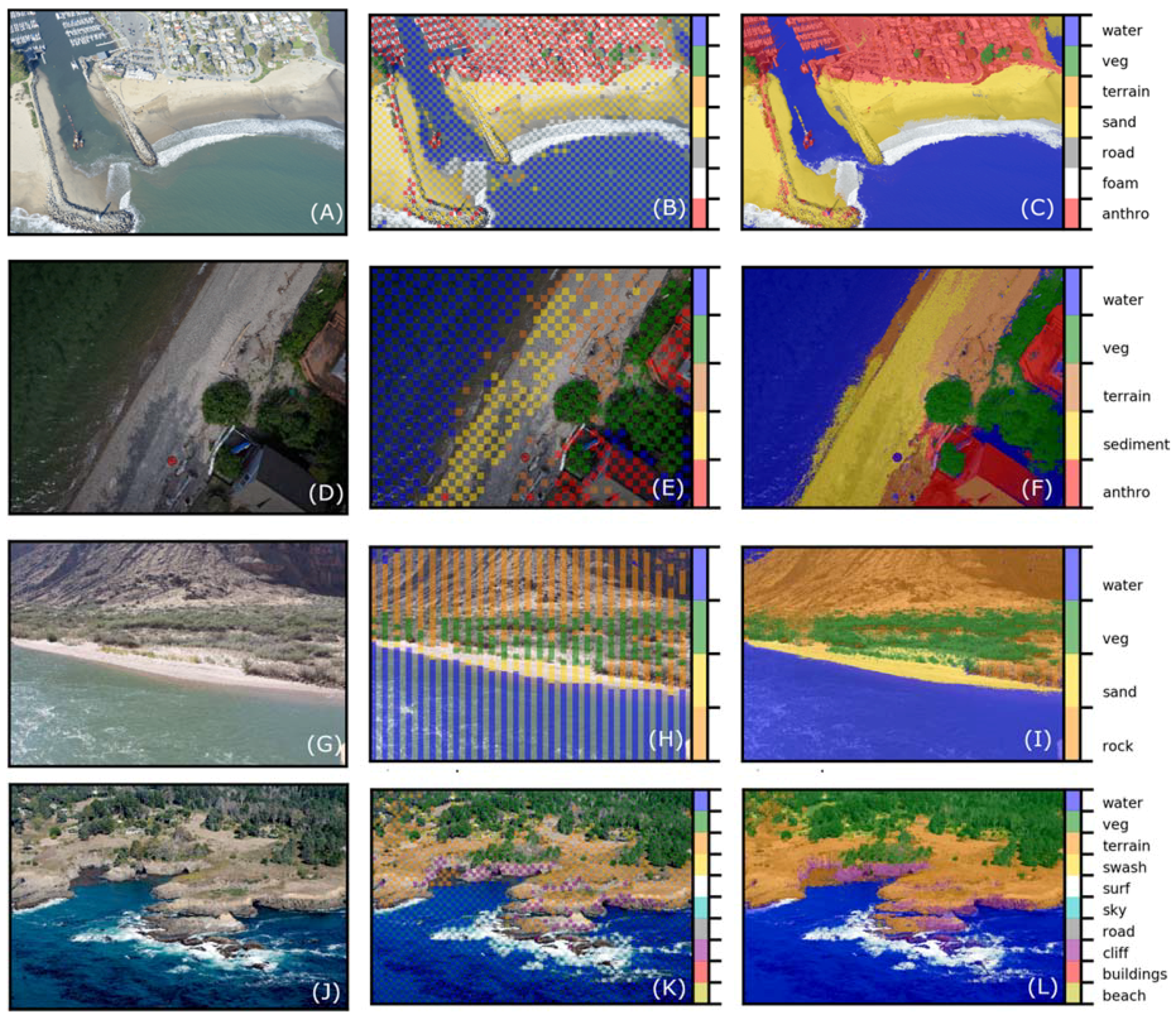
Figure 8.
Example images (A,D,G,J), DCNN-derived unary potentials (B,E,H,K), and CRF-derived pixelwise semantic segmentation (C,F,I,L) for each of the four datasets; from top to bottom: Seabright, Lake Ontario, Grand Canyon, and CCRP.
Figure 8.
Example images (A,D,G,J), DCNN-derived unary potentials (B,E,H,K), and CRF-derived pixelwise semantic segmentation (C,F,I,L) for each of the four datasets; from top to bottom: Seabright, Lake Ontario, Grand Canyon, and CCRP.

Figure 9.
Average recall versus the average area (in square pixels) of classes.

Figure 10.
Classification of a typical CCR image: (A) Original image; (B) DCNN predictions; (C) CRF predictions; (D) and (E) show the same region (2× magnification) from the DCNN and CRF labels, respectively. The colored ellipses in (D) indicate small rocky areas either misclassified (red ellipses) or correctly classified (yellow ellipses).

Table 1.
Whole tile classification accuracies and F1 scores for each dataset and tile size, using the test tile set not used to train the model.
Table 1.
Whole tile classification accuracies and F1 scores for each dataset and tile size, using the test tile set not used to train the model.
| T = 96 | T = 224 | |||
|---|---|---|---|---|
| Dataset | Mean Accuracy | Mean F1 Score | Mean Accuracy | Mean F1 Score |
| NWPU | 87% | 93% | 89% | 94% |
| Seabright | 94% | 97% | 96% | 97% |
| Ontario | 83% | 91% | 96% | 98% |
| Grand Canyon | 92% | 96% | 94% | 97% |
| CCRP | 79% | 88% | 84% | 91% |
Table 2.
Mean whole tile classification accuracies (%), per class, for each of the non-satellite datasets (T = 96/T = 224), using the test tile set not used to train the model.
Table 2.
Mean whole tile classification accuracies (%), per class, for each of the non-satellite datasets (T = 96/T = 224), using the test tile set not used to train the model.
| Seabright | Ontario | Grand Canyon | CCRP | |
|---|---|---|---|---|
| Sediment/sand | 93/98 | 76/93 | 94/89 | 91/89 |
| Terrain/rock | 91/91 | 78/91 | 89/95 | 84/78 |
| Cliff | 69/86 | |||
| Vegetation | 89/95 | 96/98 | 94/90 | 49/74 |
| Water | 99/98 | 94/97 | 92/99 | 92/91 |
| Anthropogenic | 95/98 | 72/94 | 79/85 | |
| Foam/Surf | 97/96 | 72/81 | ||
| Swash | 79/79 | |||
| Road | 96/98 | 85/83 | ||
| Sky | 90/97 |
Table 3.
Mean P/R/F/A (all %) per class for pixelwise classifications using each of the non-satellite datasets (T = 96), using the test set of label images.
Table 3.
Mean P/R/F/A (all %) per class for pixelwise classifications using each of the non-satellite datasets (T = 96), using the test set of label images.
| Seabright | Ontario | Grand Canyon | CCRP | |
|---|---|---|---|---|
| Sediment/sand | 98/92/95/92 | 72/72/74/67 | 76/79/80/78 | 84/90/86/78 |
| Terrain/rock | 44/51/46/50 | 32/32/30/41 | 80/97/87/96 | 47/86/54/75 |
| Cliff | 72/91/66/74 | |||
| Vegetation | 63/41/48/42 | 90/93/89/91 | 92/31/46/43 | 94/40/48/26 |
| Water | 95/92/93/91 | 95/95/95/89 | 94/92/93/94 | 93/88/86/79 |
| Anthropogenic | 87/95/90/94 | 78/59/64/55 | 85/70/76/71 | |
| Foam/Surf | 87/93/90/94 | 93/74/73/70 | ||
| Swash | 42/40/48/27 | |||
| Road | 86/81/83/79 | 35/70/35/64 | ||
| Sky | 95/97/94/82 | |||
| Average | 80/78/78/77 | 73/70/70/69 | 86/75/77/78 | 74/75/67/65 |
© 2018 by the authors. Licensee MDPI, Basel, Switzerland. This article is an open access article distributed under the terms and conditions of the Creative Commons Attribution (CC BY) license (http://creativecommons.org/licenses/by/4.0/).
Share and Cite
MDPI and ACS Style
Buscombe, D.; Ritchie, A.C. Landscape Classification with Deep Neural Networks. Geosciences 2018, 8, 244. https://doi.org/10.3390/geosciences8070244
AMA Style
Buscombe D, Ritchie AC. Landscape Classification with Deep Neural Networks. Geosciences. 2018; 8(7):244. https://doi.org/10.3390/geosciences8070244
Chicago/Turabian StyleBuscombe, Daniel, and Andrew C. Ritchie. 2018. "Landscape Classification with Deep Neural Networks" Geosciences 8, no. 7: 244. https://doi.org/10.3390/geosciences8070244
Note that from the first issue of 2016, this journal uses article numbers instead of page numbers. See further details here.