Vulnerability and Site Effects in Earthquake Disasters in Armenia (Colombia). I—Site Effects

Abstract

The city of Armenia, Colombia has been repeatedly subjected to moderate magnitude earthquakes. Damage in that city for the 1999 (Mw6.2) event was disproportionate (maximum observed EMS-92 intensity of IX), even considering the small epicentral distance (18 km). Two main factors have been invoked: Site effects and vulnerability of the building stock. We re-analyze available data on site effects, including: Records of aftershocks of the 1999 event, ambient noise records obtained using standalone stations, array records of ambient noise, and available shear wave profiles from seismic cone measurements. We estimate local amplification from spectral ratios of earthquake records relative to a reference site, the horizontal relative to the vertical component (HVSR, Horizontal-to-Vertical Spectral Ratios) of earthquakes and ambient noise records, and ratios of response spectra relative to a reference site or to simulated ground motion. These estimates are compared to amplification functions computed for 1D soil models, inverted from microtremor array observations. Our estimates of site effects for Armenia are therefore robust and bring together results previously available only in internal reports. We show that spectral ratios relative to a reference site may fail to estimate the amplification level. Site effects in Armenia are relatively homogeneous. Although site amplification is very significant and contributed to the observed damage, it does not account for the irregular damage distribution observed in 1999.

1. Introduction

The coffee-growing region in Colombia has been repeatedly subjected to moderate magnitude earthquakes. In the period from 1938 to 1999, eight earthquakes occurred, producing EMS-92 intensities as large as IX. The most recent event occurred very close to the city of Armenia (epicentral distance of 18 km) on 25 January 1999 (Mw6.2) [1]. This event caused 2000 casualties and 10,000 injuries due to the collapse of 15,000 houses. At least another 20,000 houses were severely damaged [2]. This is clearly too heavy a toll for a moderate size earthquake, even if the epicentral distance was small. Several institutions (e.g., Universidad del Quindío, Ingeominas) have investigated the reasons of such a disaster, but the results remain unpublished. Two main factors were detected: Site effect amplification and the exceptionally high vulnerability of the building stock. Our purpose, in this and its companion paper, is to examine the contribution of these two factors to the exceptional consequences of the 1999 event in the city of Armenia. This is important as moderate earthquakes will continue to occur in the region. Moreover, in the years since 1999, Armenia has continued growing, increasing significantly the exposed infrastructure (currently, its population is about 300,000 people). Mitigation of seismic hazards in Armenia requires a better understanding of how these two factors, site effects and vulnerability of the building stock, have contributed to past earthquake disasters.

In this paper, we address two main objectives. The first one is to integrate time results obtained from earthquake and ambient noise data, together with geology and geotechnical studies, to evaluate the significance of site effects during earthquake disasters in Armenia. Site effects are the most predictable component of a seismic hazard. Through the analysis of site effects we may be able to constrain a major factor contributing to destructive ground motion during future earthquakes [3]. Different studies have tackled site effects in Armenia (e.g., [4]). However, most of them have dealt with particular issues, and they have neither compared the results of different measurements nor integrated the different results that were presented in internal reports. Based on published results, it is not possible to decide how extensively site effects contributed to damage distribution during the 1999 earthquake. We have compiled data related to site effects that were obtained in the years since the 1999 earthquake. These data include geological and geotechnical maps, records of aftershocks from the 1999 event, and ambient noise records obtained using standalone stations and two linear arrays.

Our second objective is to review the different techniques that are currently used to estimate local amplification. These techniques are commonly used, but their results are compared only occasionally (see e.g., [5,6]). In the case of Armenia, we are able to evaluate site effects using earthquake and ambient noise data. Moreover, data on shear wave velocity structure are available from shallow seismic cone measurements at 21 sites within the city, and from the inversion of dispersion curves retrieved from the analysis of ambient noise data recorded by two linear arrays. This allows us to compare the performance of different standard techniques used to estimate local amplification, with expected site effects predicted from the inverted subsoil structure. Our results show, in general, very good agreement among the different techniques.

2. Setting

Armenia is a medium sized city located in the coffee growing region of Colombia, 290 km to the West of Bogota, at an altitude of 1500 m. It houses currently about 300,000 people. The surface geology of the region is shown in Figure 1, together with the location of Armenia (irregular white shape), neighboring towns, and main rivers. Surface geology includes metamorphic, igneous, and sedimentary rocks. The line, AA’, crossing Armenia in Figure 1 shows the location of the geological cross-section across the city, shown in Figure 2. In contrast with the complex regional geology shown in Figure 1, the geology under Armenia is relatively simple. The geologic bedrock are metamorphic rocks. Along the Quindio river, fluvial volcanic deposits have been identified, but are absent under Armenia. In the city, on top of the metamorphic rocks, different sequences of volcaniclastic deposits (Tertiary) overlay the bedrock. Weathering of these deposits have resulted in about 8 to 12 m of silt and silty clay that overlay them. Highly weathered deposits of volcanic ash (about 7 m thick, not shown in Figure 2) are the surface deposits for most of the city, frequently cut by gullies as the soft ash deposits are easily eroded by rain. Some of the gullies have been filled by anthropic deposits. As shown in Figure 2, the basic stratigraphy in the city is relatively constant and the thicker layer, the volcaniclastic deposits, is basically horizontal, with an approximately constant thickness. The cross-section shows two normal faults. However, their throw is small relative to the thickness of the layers.

3. Data and Techniques of Analysis Used

3.1. Earthquake Data

After the occurrence of the 1999 earthquake, a temporary array of five strong motion stations (Kinemetrics Etna or K2 recorders coupled to FBA accelerometers) was deployed to record aftershocks (six stations in total, considering the permanent station at UNI, located at Quindio University). Nine aftershocks were recorded by at least two stations (relevant data are given in

Table 1. Epicentral coordinates of the nine aftershocks analyzed. The last column indicates the stations that recorded each event.

#	Date	ML	Depth	Longitude W	Latitude N	Stations
1	5 May 1999	3.0	5.0	75.70	4.52	CAL, CAR, CSD, VIV, UNI, EST
2	7 May 1999	2.8	19.3	75.62	4.46	CAL, VIV, EST
3	15 May 1999	2.4	22.1	75.61	4.43	CAL, VIV, EST
4	16 May 1999	2.7	14.7	75.65	4.45	CAL, CAR, VIV, EST
5	16 May 1999	2.9	11.9	75.69	4.46	CAL, CAR
6	23 May 1999	3.1	11.7	75.72	4.51	CAL, CSD
7	12 October 1999	4.1	6.7	75.68	4.32	CAL, UNI
8	21 October 1999	3.5	8.0	75.63	4.47	CAL, UNI
9	9 November 1999	3.8	9.9	75.59	4.43	CAL, UNI

; epicenters are plotted in Figure 3). Recorded Peak Ground Acceleration (PGA) varies between 0.34 gal (for event 3, recorded at CAL) and 20.8 gal (for event 7, recorded at CAL). Clearly, such small PGA indicate that we can safely rule out any possible non-linearity. Figure 4 shows an example of the data. The three acceleration components recorded at stations CAL and UNI for event 7 (Table 1) are shown on the left. The right diagrams show Fourier amplitude spectra. We observe a strong contrast in both time and frequency domains. The records at CAL exhibit simple traces with small durations. The records at UNI show more significant low frequency ground motion and much larger durations. Station CAL is located on heavily weathered metamorphic rocks, classified as saprolite (Figure 1). This station is the closest we may get to a station on rock close to Armenia and thus it was chosen as the reference station. We are aware that the weathered layer may produce site effects, but we expect that the thickness of the weathered layer will be small and site effects, if present at CAL, will occur at high frequencies.

We evaluated site effects from our aftershock records using three different techniques: Spectral ratios relative to a reference site (SSR), spectral ratios of the horizontal relative to the vertical component (HVSR), and response spectral ratios (RSR). SSR [7,8] is often considered the most reliable technique to estimate site effects. Indeed, when we compare two seismic records produced by the same seismic source and propagated through roughly the same path, SSR gives a reliable estimate of local amplification, provided that one of the records was obtained on intact rock on flat terrain, which is, by definition, free of local amplification. Unfortunately, a rock site close to the location where we need to estimate site effects does not always exist. Moreover, a very large scatter of the results seems irreducible (see for example [9]). Therefore, the statement that SSR is the most reliable standard against which all other estimates are evaluated against may be questioned. It is for this reason that we used our earthquake data to estimate site effects using additional techniques.

Earthquake HVSR [10,11,12] have been proposed to estimate local amplification. This technique was shown to provide reliable estimates of site effects by [13] except where vertical amplification is not negligible. However, even in this case, F. J. Chávez et al. (2014) [14] showed that the HVSR of earthquake data may still be useful because a possible amplification peak in the vertical component (at a frequency that is proportional to P-wave velocity, if the peak is associated to vertical propagation of P waves) will necessarily appear at frequencies higher than the amplification peak in the horizontal components (at a frequency proportional to S-wave velocity, if the peak is associated to vertical propagation of S waves). At worst, the amplification level will be underestimated. R. R. Castro et al. (2014) [13] observed that earthquake HVSR and microtremor HVSR can be used to estimate a reliable fundamental frequency, but microtremor HVSR may overestimate the maximum amplification relative to earthquake HVSR.

Response spectral ratios (RSR) were proposed in [15] as a means to predict expected response spectra at soft soil sites for a future event from the response spectra estimated on firm ground. Those authors showed that RSR could also be used to estimate local amplification by comparing RSR with SSR. RSR involve a non-linear operation and therefore cannot be interpreted as transfer functions in the sense of Fourier amplitude spectral ratios. However, despite the substantial smoothing introduced by convolution of the earthquake record with the impulse response of a single degree of freedom oscillator, E. Rosemblueth et al. (2012) [15] observed that RSR are a very good estimate of the average site response estimated from SSR. Similar results have been presented more recently in [16]. We have computed RSR using station CAL as the reference, as we did for SSR.

In addition to computing RSR using station CAL as the reference, we estimated local amplification from response spectral ratios using a different reference. C. E. Hruby et al. (2003) [17] proposed to estimate site amplification using spectral ratios between earthquake records and the Fourier amplitude estimated at the site from the finite-fault stochastic ground-motion simulation model. This is a hybrid estimate of the site amplification in that the reference Fourier amplitude spectrum is computed using the stochastic model. C. E. Hruby et al. (2003) [17] proposed the use of the transfer functions estimated in this way as empirical corrections to ground motion predictions using the stochastic method. Following the same line of thought, D. Motazedian et al. (2005) [18] and G. Atkinson et al. (2013) [19] proposed to estimate local site effects as the difference between observed response spectra and the ground motion prediction equations developed by [20]. Again, site response is estimated as ratios of response spectra between observed records and response spectra predicted by the ground motion prediction model. In this paper, we have used the stochastic method, following the detailed description given in [21]. The method combines a parametric description of the ground motion’s amplitude spectrum with a random phase spectrum, modified such that the motion is distributed over a duration related to the earthquake magnitude and to the distance from the source. It is assumed that the far-field accelerations on an elastic half space are band-limited, finite-duration, white Gaussian noise, and that the source spectra are described by a single corner-frequency model whose corner frequency depends on earthquake size (the ω-square model [21]). The amplitude spectrum of the source model is modified by geometric expansion and anelastic attenuation for the path source-receiver (a homogeneous halfspace is assumed with Q = 275). The reference response spectra on rock (without site effects) at the site where ground motion is modelled is obtained using random-vibration theory. We use these computed response spectra as a reference to estimate local amplification from response spectra computed for our earthquake records.

Our results for SSR and HVSR were computed using Fourier amplitudes of the whole records, smoothed using the window proposed in [22], with a b-parameter of 40. As a check for the stability of the results, we also computed our ratios using a shorter window (10 s duration), selecting only the largest amplitudes in each accelerogram. Finally, in addition to smoothed Fourier amplitude spectra, we computed again spectral ratios for earthquake data from spectral amplitudes estimated using singular spectrum analysis [23,24,25,26]. Our results remained unchanged.

3.2. Ambient Noise Data

The use of ambient noise records is very common in current site effect studies. The ease with which records can be obtained and analyzed makes ambient noise a very popular tool to estimate local amplification, even if good results are not always obtained. In this paper, we have used the standard HVSR of seismic noise records [27,28] to estimate site effects. HVSR of ambient noise is recognized as a valuable tool to identify possible resonance frequencies where the subsoil structure is relatively simple (e.g., [5,6,11,28]). The possibility of using the corresponding amplitude to estimate local amplification is more controversial, with good results at some places (e.g., [29,30]) and insufficient at others (e.g., [31,32]). In this project, we recovered the HVSR of ambient noise measurements made at 29 points in Armenia in 2002. A DR100 digital recorder by Sprengnether, coupled to three 5-s seismometers by Kinemetrics, was used to record between three and five minutes of ambient vibration at each site. The windows for analysis were selected from the records visually, without using an anti-triggering algorithm. Fourier amplitude of 20-s windows, smoothed using a one third octave square window (similar to the standard smoothing window of [22]), were used to estimate average HVSR from three to five windows at each site.

In addition to those old measurements, in August 2017, additional ambient noise records were obtained at the six sites where the aftershocks of the 1999 event were recorded. Two different instruments were deployed simultaneously at each site: A Kinemetrics Basalt recorder coupled to an FBA episensor accelerometer and a Nanometrics Taurus recorder coupled to a Trillium broad band, 120 s seismometer. At each site, one to three hours of ambient noise was recorded, and therefore the instruments had ample time to stabilize. Processing followed standard lines, similar to those used for the earthquake data. One-minute windows with 50% overlap were selected from the records. The mean and linear trend were removed and a Hanning taper was applied to each end of the window over 5% of its duration. For each station, between 200 and 300 noise windows were processed. Each HVSR was smoothed using again the window proposed in [22], with a b-parameter of 40, and the results were averaged for all windows at each site.

Finally, array measurements of microtremors were used at two sites close to Armenia (PE and HA in Figure 3). This experiment, carried out in June 2012, was designed with the aim of retrieving a shear-wave profile down to bedrock depth. At each of those two sites, five instruments were used to record seismic noise (Taurus digitizers coupled to broad band Trillium seismometers by Nanometrics). The geometry of the array was linear, with five different spacing between neighboring stations: 5, 10, 20, 40, and 80 m. Thus, the total length of the linear array varied from 20 to 320 m. This choice forced us to make these measurements out of Armenia; a crowded city where it was not possible to find a suitable location for these long arrays. For each configuration, 3 h of seismic noise was recorded. The vertical component of these data was analyzed using the spatial autocorrelation (SPAC) method [33,34], computing cross-correlation between every station pair recording simultaneously in the frequency domain [35,36]. Aki, K. (1957) [33] defined correlation coefficients as the averaged, normalized cross-correlation of ambient noise at a fixed distance as a function of frequency (see also [34,35,36]). According to the theory of the SPAC method, correlation coefficients should take the form of a Bessel function of first class and order zero. Its argument is frequency times the distance between stations divided by the phase velocity (of Rayleigh waves for the case of cross-correlation of vertical components). We computed results from SPAC using two different paths. The first was to use the procedure detailed in [35]. For each inter-station distance, we selected several hundred 4-min windows of ambient noise from the simultaneous records. Each window of noise had its mean and linear trend removed and a Hanning taper was applied to each edge over 5% of its duration. Cross-correlation was computed between two stations for 64 frequencies distributed logarithmically between 0.1 Hz and 40 Hz, and an average of the normalized cross-correlation was computed for each station pair. These correlation coefficients were inverted to minimize their difference with a Bessel function of first class and order zero, and phase velocity values as a function of frequency were estimated from the argument of the Bessel function. Finally, the phase velocity dispersion curve was inverted to estimate a shear-wave velocity profile using a linearized version of the stochastic least square method [35]. In addition to this procedure, we repeated the analysis using the SPAC method, with the program suite proposed in [37]. GEOPSY uses the same procedure to analyze ambient noise data, but the estimation of correlation coefficients and their inversion to estimate a subsoil profile are different. For example, phase velocity dispersion curves are inverted using the neighborhood algorithm [37]. The data, procedures, and results at one of the two sites analyzed using GEOPSY were presented in [38]. We verified that the final results of the SPAC method were the same using the two different processing procedures.

4. Results

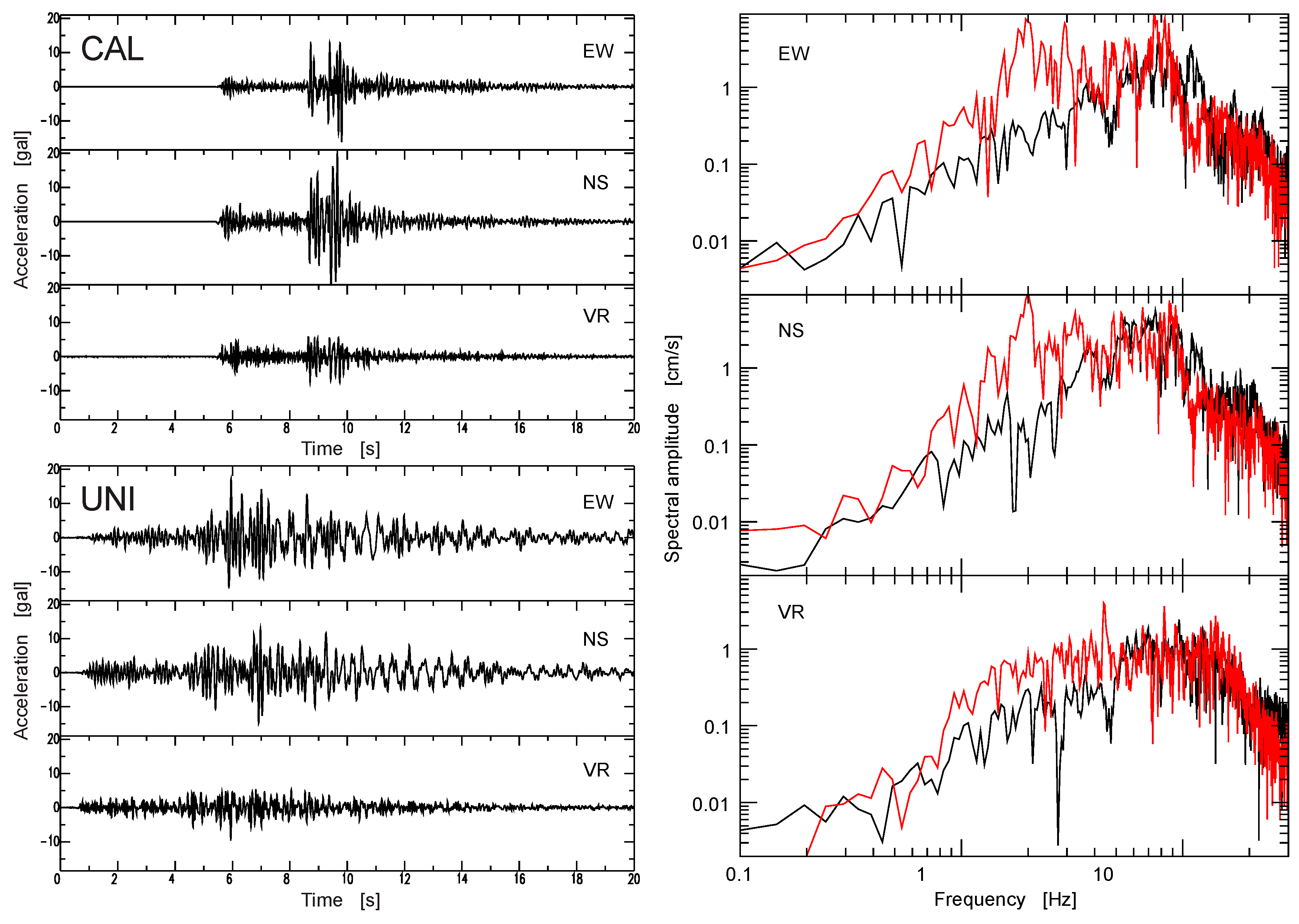
Fourier amplitude spectra computed for our earthquake records were used to estimate amplification using SSR and HVSR. A time window of 20 s was used. For many events, this comprised the complete records (e.g., Figure 4). The traces had their average value removed, as well as any possible linear trend in the record. A Hanning taper over 5% of the window duration was applied at each end. Fourier amplitude spectra were smoothed using the window proposed in [22], with a b-parameter of 40. 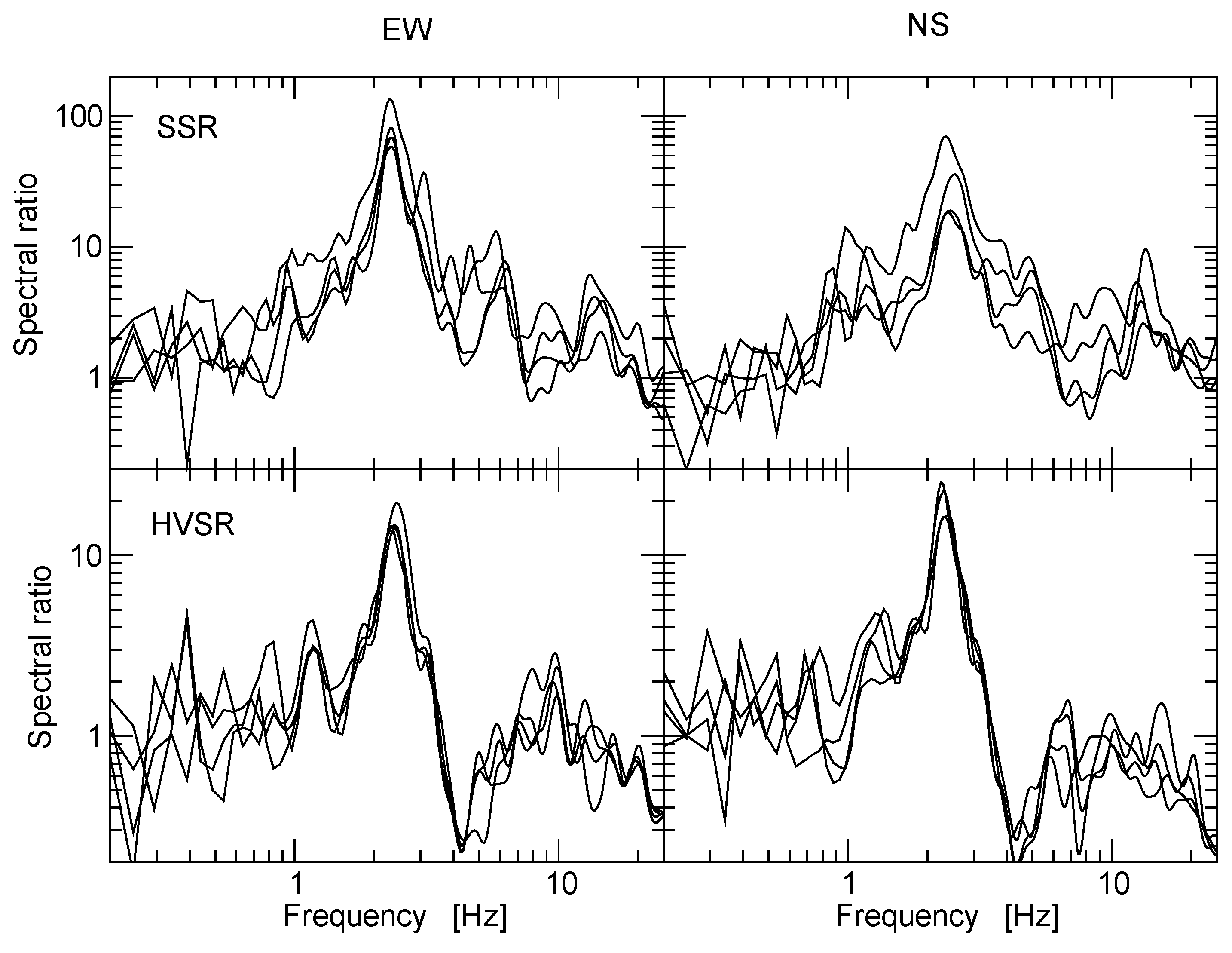Figure 5 shows an example of the results. This figure shows SSR and HVSR for the four aftershocks recorded by station EST. Station CAL is the reference station for SSR. A very prominent amplification peak is observed between 2 Hz and 3 Hz for both SSR and HVSR. The shapes of the curves are very similar for both techniques. However, amplitudes of SSR transfer functions are almost an order of magnitude larger than the results for HVSR. That is, station CAL seems not to be affected by a local amplification function that would affect the shape of the SSR, but its amplitudes are small and, consequently, SSR relative to CAL have large amplitudes. Earthquake HVSR curves show a smaller scatter than SSR curves, giving a more precise image of the transfer function at EST.

SSR requires that the propagation path be similar between the source and the soft soil and reference sites. This may not be satisfied in our data (Figure 3) given the short epicentral distances and the consequent azimuth differences between the source and recording stations. We corrected Fourier amplitude spectra for geometrical spreading and recomputed SSR. The scatter among SSR curves for each station did not decrease and, at some stations, increased significantly (therefore, results shown correspond to SSR uncorrected by geometrical spreading). We conclude that even small location errors may significantly change the computed epicentral distances and azimuths for aftershocks that were recorded at distances as small as 1.1 km. Clearly, SSR indicates that site effects are very significant. However, this technique is unable to provide a precise estimate of amplification because amplitudes of ground motion recorded at CAL seem to be unnaturally small, by a factor that is independent of frequency. A possible explanation would be large differences in the radiation pattern from the source to CAL relative to our other stations.

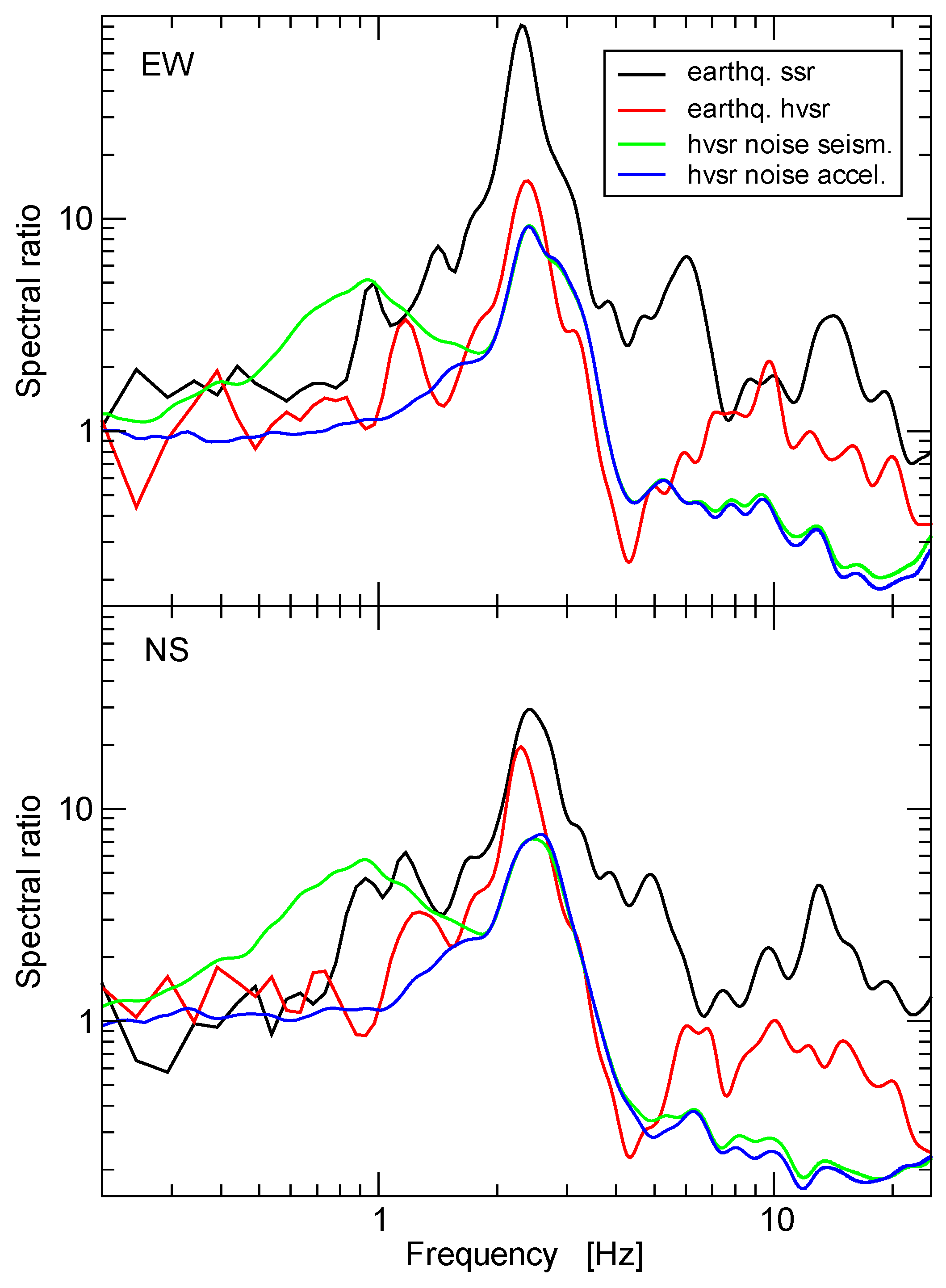
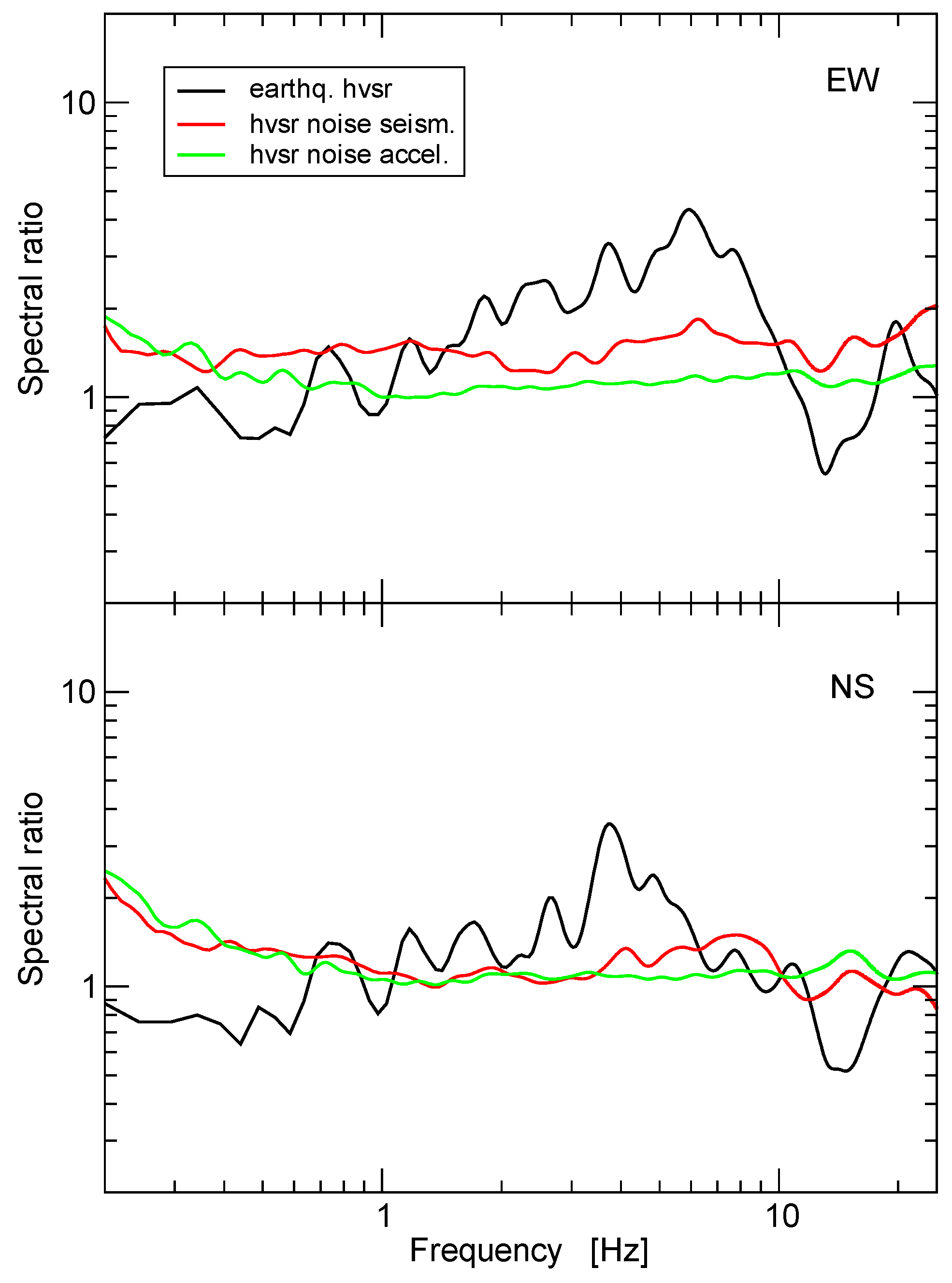
Average results for station EST are shown in Figure 6. This figure shows average earthquake SSR and HVSR results together. Two additional curves in this figure show the results of HVSR of ambient noise recorded at station EST using the broad band seismometer and the FBA accelerometer. Results for ambient noise indicate that there are some differences between the seismograph and the accelerograph records. However, they appear at frequencies below 2 Hz, outside the frequency range where ground motion is amplified at this site. For frequencies above 2 Hz, the results for seismic noise recorded using a seismograph or an accelerograph are undistinguishable (the same was observed for all other five stations). All the curves in Figure 6 show a large amplification peak between 2 Hz and 3 Hz. However, the amplitudes display a large scatter, between 9 and 80 for the EW component and between 7 and 30 for the NS component. Earthquake data SSR show larger amplification than all other estimates. Earthquake data HVSR are closer to amplification estimates from ambient noise data, which show the smallest amplitudes of the resonant peak. However, it is well known (e.g., [28,31]) that HVSR of ambient noise usually underestimate local amplification. For this reason, we qualify the results in Figure 6 as in good agreement, despite the small differences between HVSR of earthquake and ambient noise data.

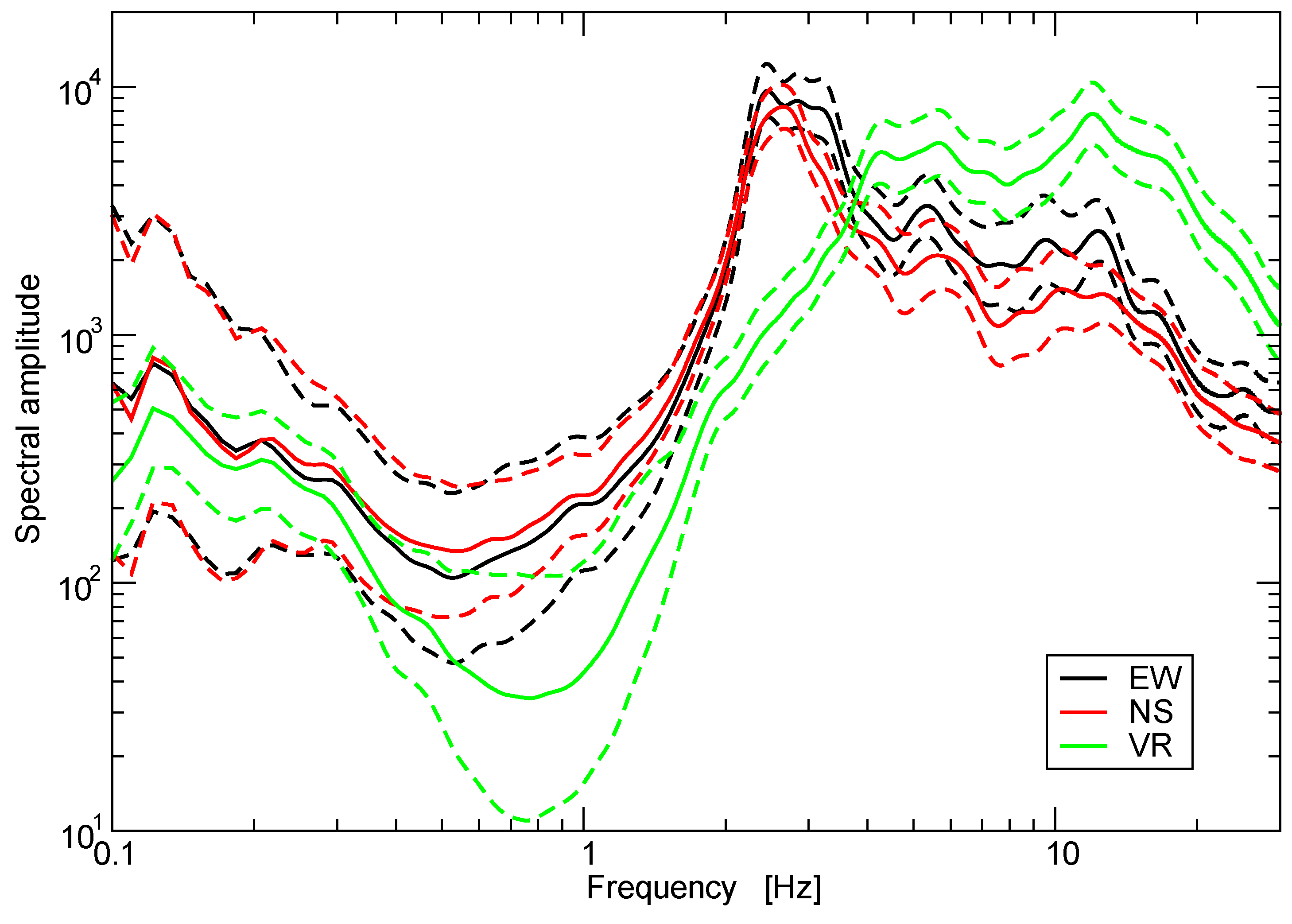
In addition to the resonance peak between 2 Hz and 3 Hz, broad band seismograph HVSR in Figure 6 show a broad, smaller amplitude peak at about 1 Hz. This peak is absent from the earthquake data curves and from accelerometer ambient noise HVSR. Figure 7 shows average Fourier amplitude spectra of ambient noise recorded at station EST using the broad band seismometer (average for 236 windows of 60 s duration). Solid lines show average values. The dashed lines indicate average plus or minus one standard deviation. The broad peak at 1 Hz results from anomalous low amplitude of the vertical component. However, the resonant peak between 2 Hz and 3 Hz stands out in both horizontal components and the three components show very small scatter in that frequency range.

The results shown in Figure 5 and Figure 6 show that SSR computed using CAL as a reference station estimates correctly the fundamental frequency, but overestimates significantly the maximum amplification by a factor that seems independent of frequency. Figure 8 shows HVSR results for CAL using both earthquake and ambient noise data. Results for ambient noise do not show evidence of sub-surface resonance, in terms of HVSR peak frequencies. The weak-motion HVSR show some small amplification between 3 and 8 Hz, which is in good agreement with the geological description of the site at this station (a thin weathered layer overlying metamorphic rock). This indicates that SSR does not fail to provide a precise estimate of site effects in Armenia because of local resonances at CAL. We hypothesize that because the source locations are close to the recording stations, differences in radiation pattern decrease significantly the amplitudes of the earthquake recorded at station CAL. Unfortunately, we do not have the data to test this hypothesis.

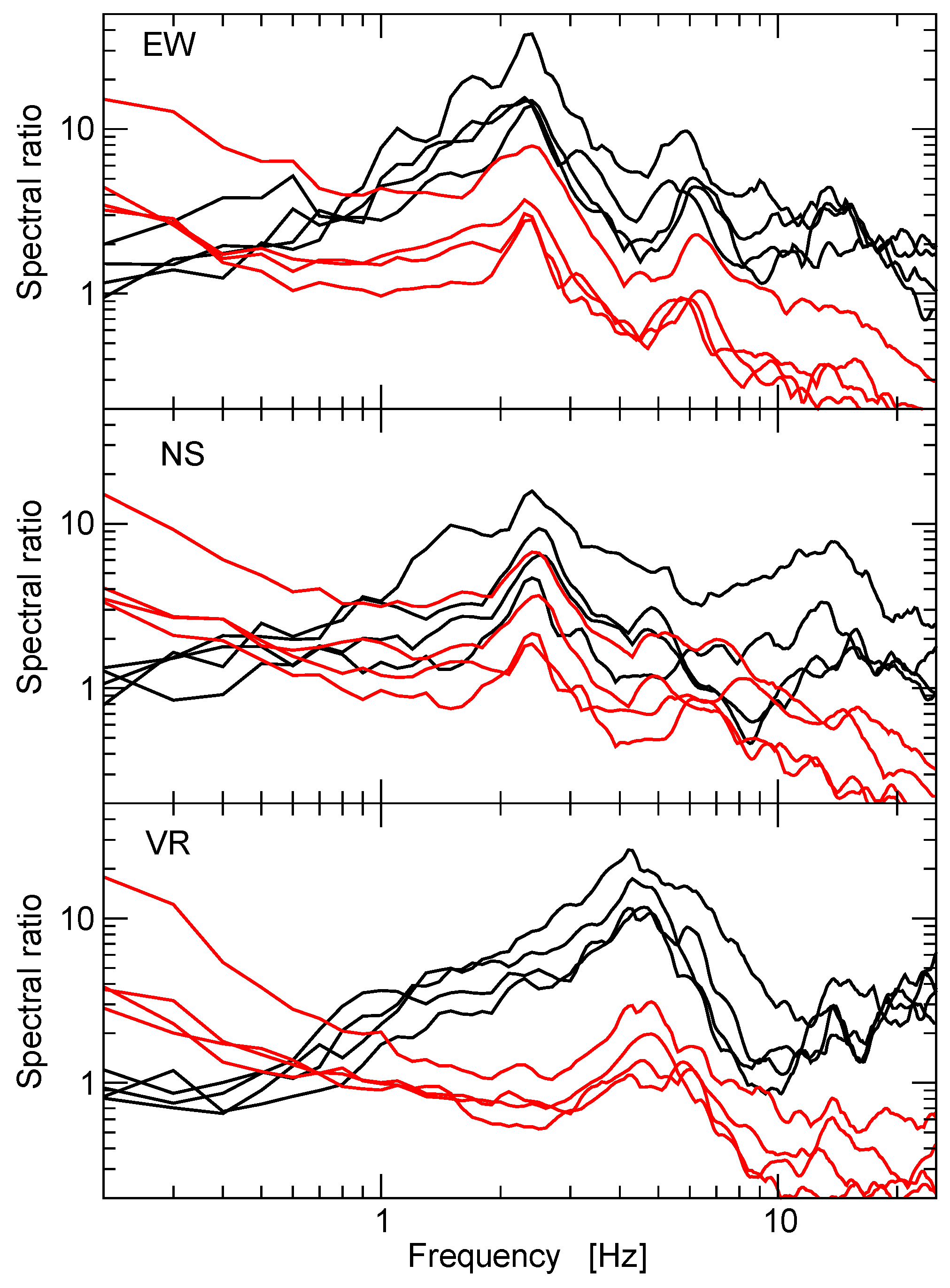
Figure 9 shows results computed using response spectra. For each aftershock, black solid lines show the ratios of response spectra computed for the records at station EST divided by the corresponding response spectra of the records at the reference station, CAL. As mentioned above for SSR, we did not correct for geometric expansion as this correction did not improve the results. We also computed ratios of response spectra, using as the reference the predicted response spectra at each site computed using the program, SMSIM (see the detailed description in [39,40]). For each earthquake record, we simulated the response spectrum predicted by the stochastic method using a point source ω-square model and varying only the magnitude and distance. A factor of 0.71 is used to account for the partitioning of energy into two horizontal components, and an average radiation factor of 0.55 is assumed. The red lines in Figure 9 show RSR relative to the SMSIM simulated response spectra. The shape of the estimated amplification functions are very similar between the black and red lines. Both predict an amplification peak at a frequency that is very similar to that obtained from SSR. Moreover, RSR relative to CAL show very similar amplitudes with those obtained using earthquake HVSR. Results for the vertical component indicate amplification at a frequency that is larger by about a factor of 2 relative to the frequency for which we observe amplification of the horizontal components in Figure 9. This is to be expected if amplification for both vertical and horizontal components is produced by the velocity contrast for the P and S wave velocities (Vp and Vs) at the base of a single layer over the halfspace model (assuming vertical plane wave incidence). The ratio between fundamental frequencies for vertical and horizontal ground motion corresponds in that model to the ratio between Vp and Vs. The amplitude of amplification of RSR relative to CAL is significantly different from that observed in the ratios of response spectra relative to SMSIM predictions, which are very small. This suggests that SMSIM simulations overestimate response spectra at CAL, which is consistent with the hypothesis stated above of a small radiation pattern affecting records at CAL. In addition to a frequency independent difference between the black and red lines in Figure 9, we observe that the red lines decrease faster with frequency than the black lines at high frequencies. This suggests that SMSIM simulations underestimate anelastic attenuation along the path source-receiver.

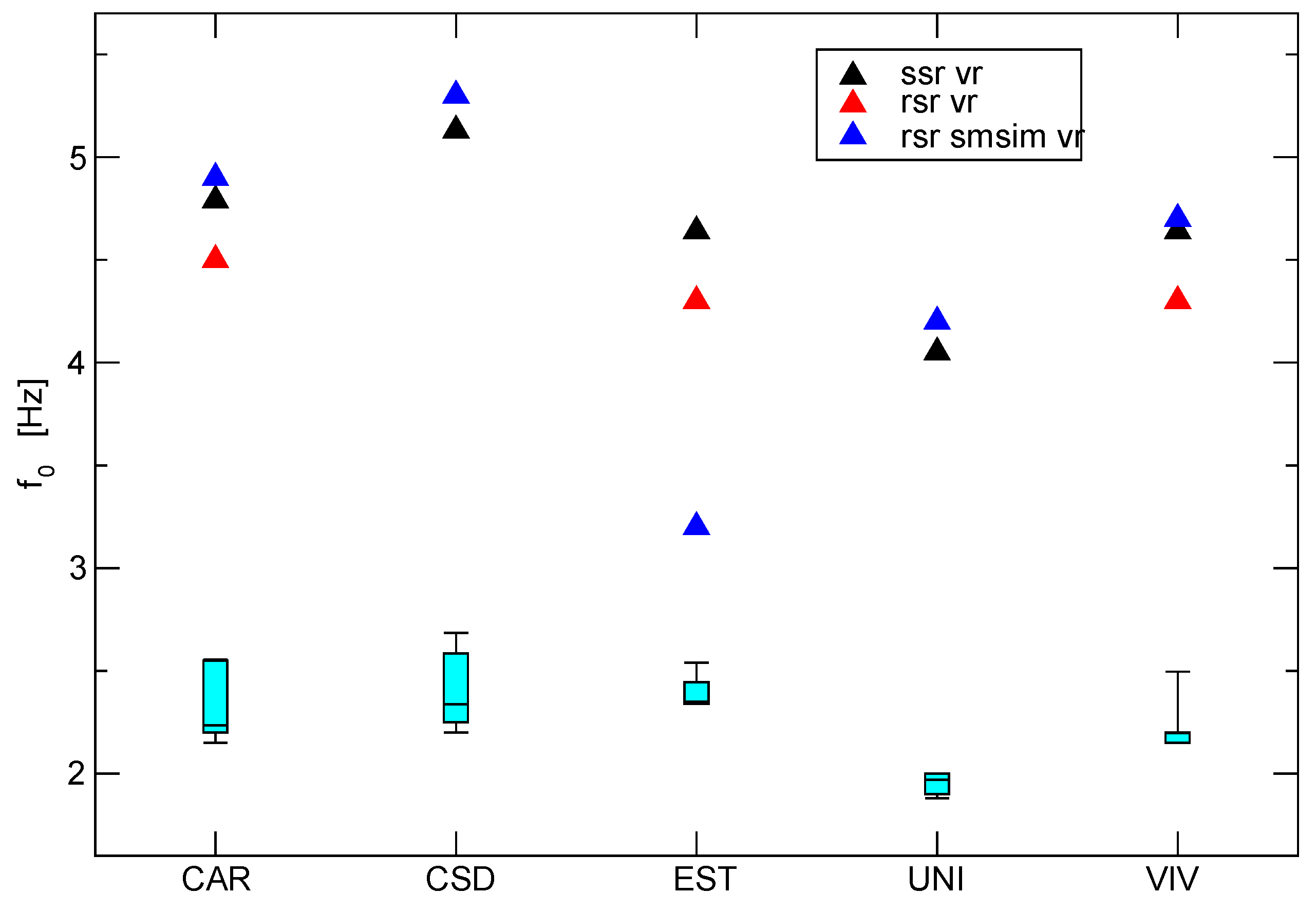
Let us now compare the values of fundamental frequency estimated at the five instrumented sites inside Armenia. Figure 10 shows together the fundamental frequency values for horizontal and vertical components obtained from our different estimates of site response using a standard box plot. We averaged together the NS and EW components for each estimate. We observe very small variations throughout the city, as fundamental frequencies for horizontal ground motion vary less than 0.5 Hz. The differences in horizontal fundamental frequency among the five stations are echoed by the vertical component fundamental frequencies, where variations are larger, but of the same order as those for the horizontal component (about 20%). For the vertical component, it is only the estimate obtained from the ratios of observed response spectra relative to the response spectra, simulated using SMSIM at station EST, that diverges from the other estimates. A Poisson ratio of 0.25 implies a factor between Vp and Vs of $\sqrt{3}$. The differences between the fundamental frequencies in the horizontal and vertical components suggest a ratio between Vp and Vs of the order of a factor 2, indicating a Poisson ratio in the layer at the origin of the amplification slightly larger than 0.25.

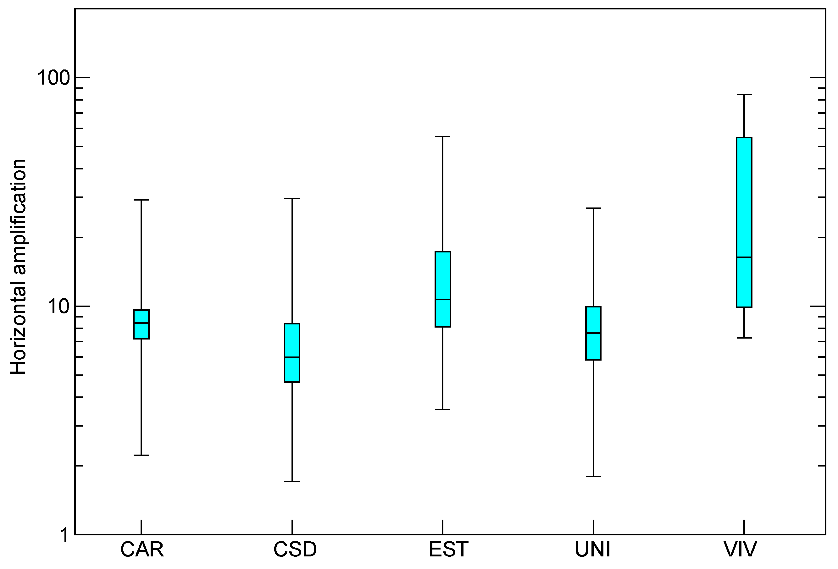
Similar to Figure 10, Figure 11 compiles horizontal amplification from the different techniques used to estimate site response, again using a box plot. As expected, the scatter is significantly larger than that for the fundamental frequency. The median value varies between 6 for CSD and 16.4 for VIV, a variation slightly larger than the usual uncertainty factor of 2 [8,41,42]. This suggests that maximum amplification shows mild variations in Armenia. The upper extreme values correspond to SSR for all the stations, and, as stated above, they may be biased by unnaturally small amplitudes at the reference station CAL. If we make an abstraction of the upper and lower extreme values, the maximum amplification in Armenia may be considered relatively constant, around a factor of 8 or 9, and would have an associated uncertainty smaller than a factor of 2.

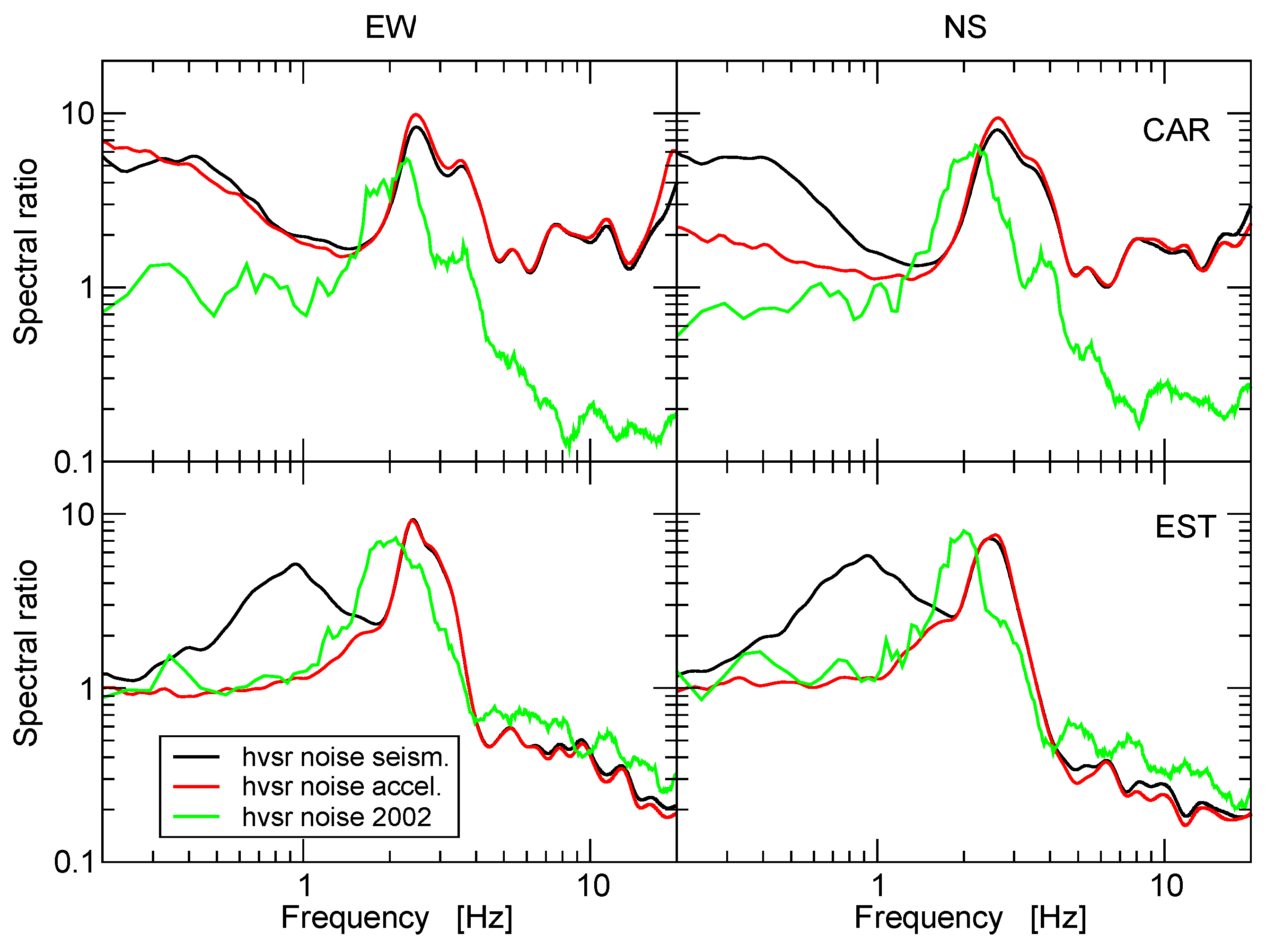
The results for the aftershocks suggest that site response does not vary significantly within Armenia. However, earthquake data gives us information on site response only at five sites. Consider now the additional ambient noise measurements made at 29 sites within the city in 2002. As a different instrument was used, it is first necessary to compare the 2002 measurements with those made recently at the five sites where aftershocks were recorded. Figure 12 shows this comparison for two stations, CAR and EST. Together with the results for HVSR from ambient noise recorded during August 2017, we plot the results of HVSR at the closest points, measured in 2002 using the Sprengnether DR100 and 5-s period seismometers. We would have preferred to compare measurements at exactly the same location. Unfortunately, in 2017, we borrowed the instruments used, which were returned to their owner before we had the map with the locations of the sites measured in 2002. The distance between CAR and point P27 is 87 m, while that between EST and P14 is 582 m. The fundamental frequency value varies a little between measurements made in 2002 and 2017. However, the difference are small in both cases, and are larger between EST and P14 than between CAR and P27, in agreement with the corresponding distances between the measurement points. The maximum amplitudes of HVSR are very similar. This suggests that it is possible to add the results of the measurements made in 2002 to those obtained at the five accelerographic stations.

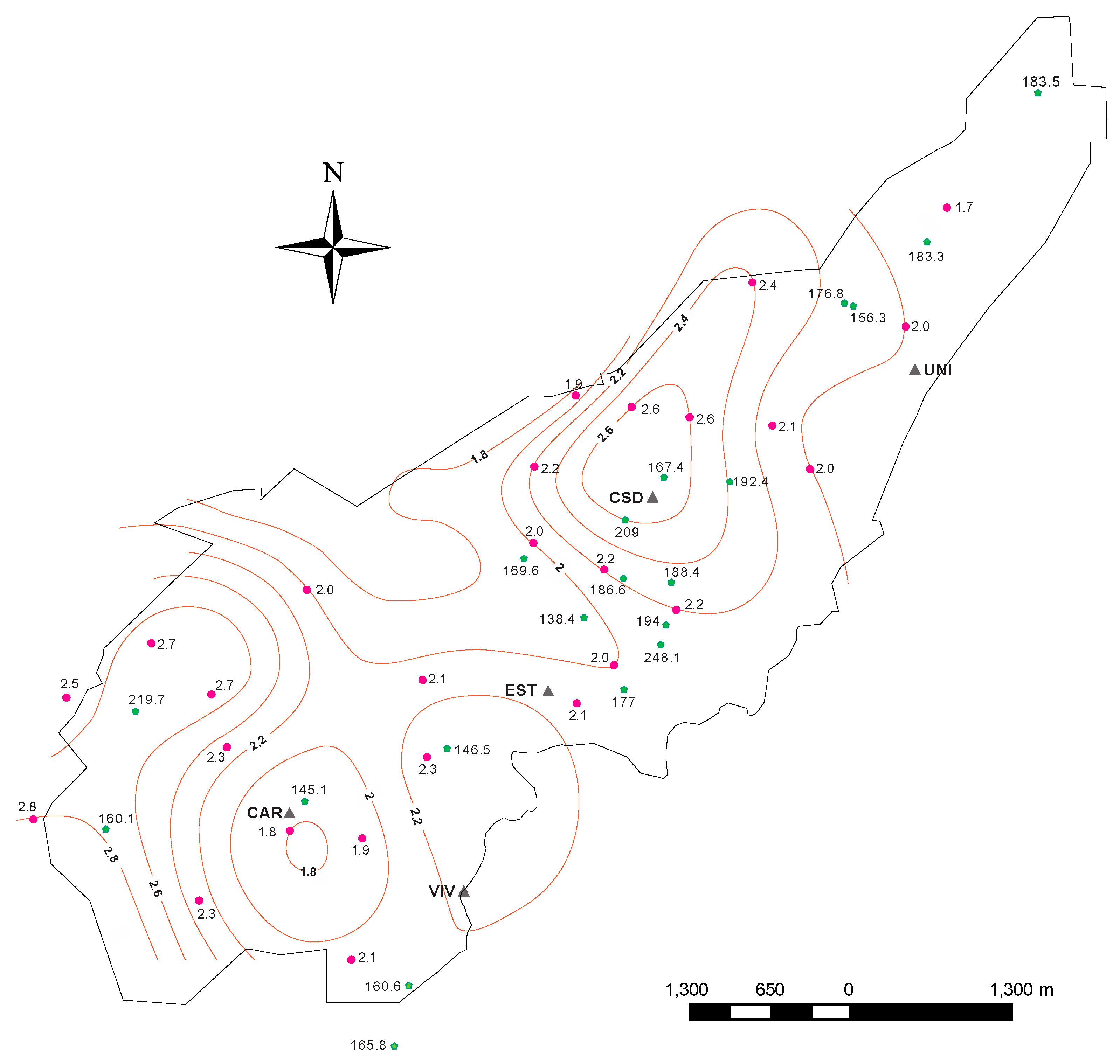
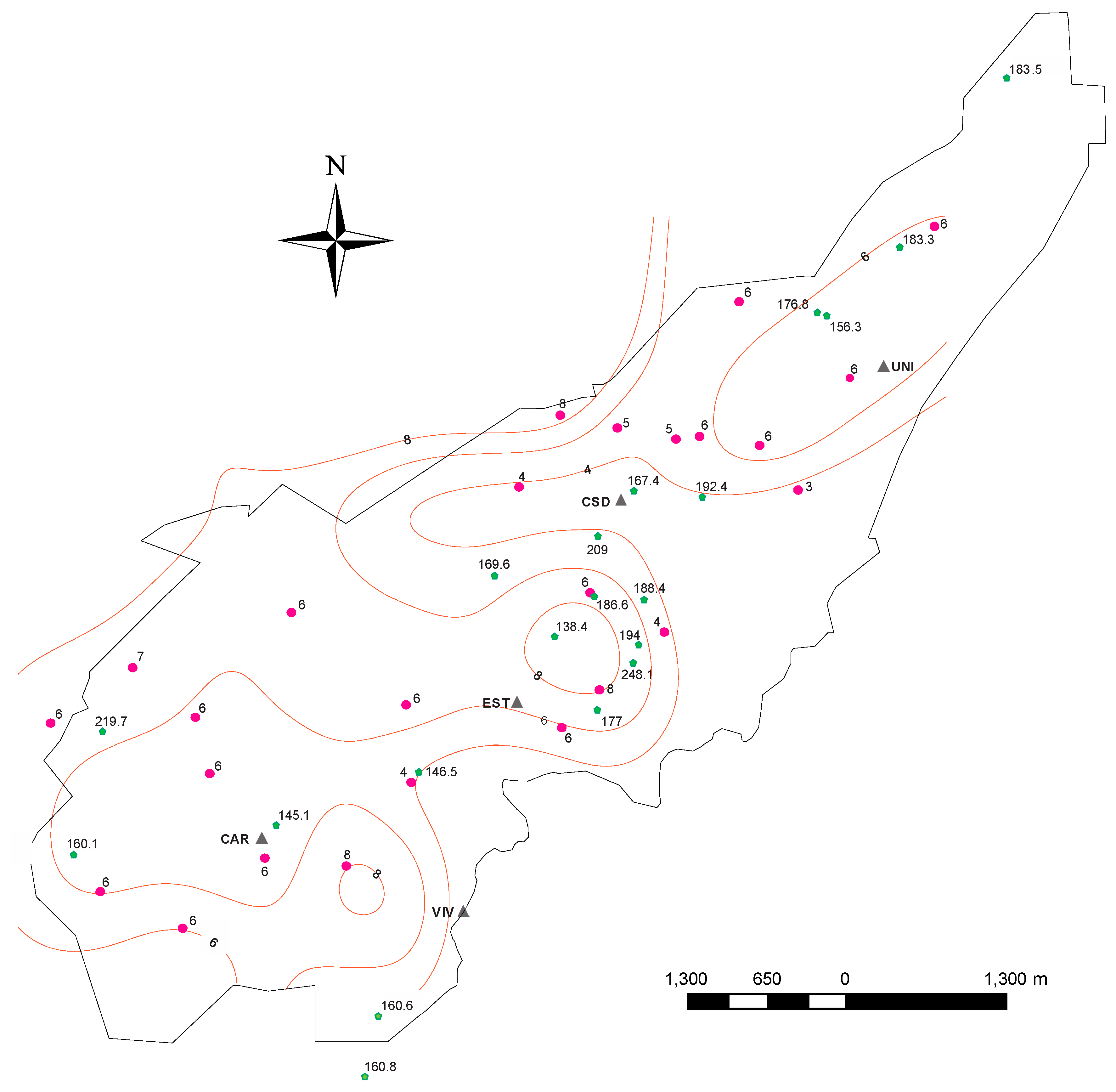
Figure 13 shows the final map of the fundamental frequency obtained from HVSR of ambient noise. Fundamental frequency within the city varies between 1.7 Hz and 2.8 Hz. The corresponding contours of the maximum amplification, computed as the average for both horizontal components, are shown in Figure 14. The observed amplification varies between 4 and 8 (only a single point shows an amplification of 3). These values are somewhat smaller than those shown in Figure 11. However, it is well known (e.g., [28,31]) that ambient noise HVSR underestimate local amplification relative to that estimated using earthquake data. Thus, we may consider that Figure 11 and Figure 14 show very good agreement. The shape of the contours in Figure 14 shows no relation with that of the contours in Figure 13. Figure 13 and Figure 14 also show the values of average velocity determined at 21 sites within Armenia using the seismic cone, in the frame of a microzonification project. The depth of investigation varied between 11 m and 30 m, with an average depth of 17 m, and, therefore, these measurements sample only the shallowest layers. We averaged the results at each site using the relation:

$$Vs=\frac{{{\displaystyle \sum }}_i^n{h}_i}{{{\displaystyle \sum }}_i^n\frac{h_i}{V_{si}}}$$

where h_i and V_si are the thickness and shear wave velocity of the n-layers determined at each site, and Vs is the average shear wave velocity, indicated at each measurement point in Figure 13 and Figure 14. Average shear wave velocities varied between 140 m/s and 250 m/s. However, we observe no relation between these values and the contours of the maximum amplification, or between those values and the contours of the fundamental frequency. Fundamental frequency is closely related with the average shear wave velocity of the soft layers and their thickness. The fact that contours of the fundamental frequency show no relation with the distribution of Vs determined from seismic cone tests suggests that shallow Vs values do not reflect the average shear wave velocity for the thickness of sediments at the origin of the fundamental frequency value. This is supported by the lack of correlation between the contours of maximum amplification and the same Vs values. Amplification is related to impedance contrast at the base of the sedimentary layers. If the variations in shallow Vs were representative of Vs for the sedimentary layers at the origin of site effects, we should observe some correlation of those Vs values with the contours of maximum amplification. Figure 13 and Figure 14 suggest together that shallow variations of Vs are not representative of the average velocity for the sedimentary layers at the origin of site effects, that those sedimentary layers have a rather homogeneous average Vs, and that the impedance contrast between average Vs for the soft deposits and the underlying bedrock is relatively constant.

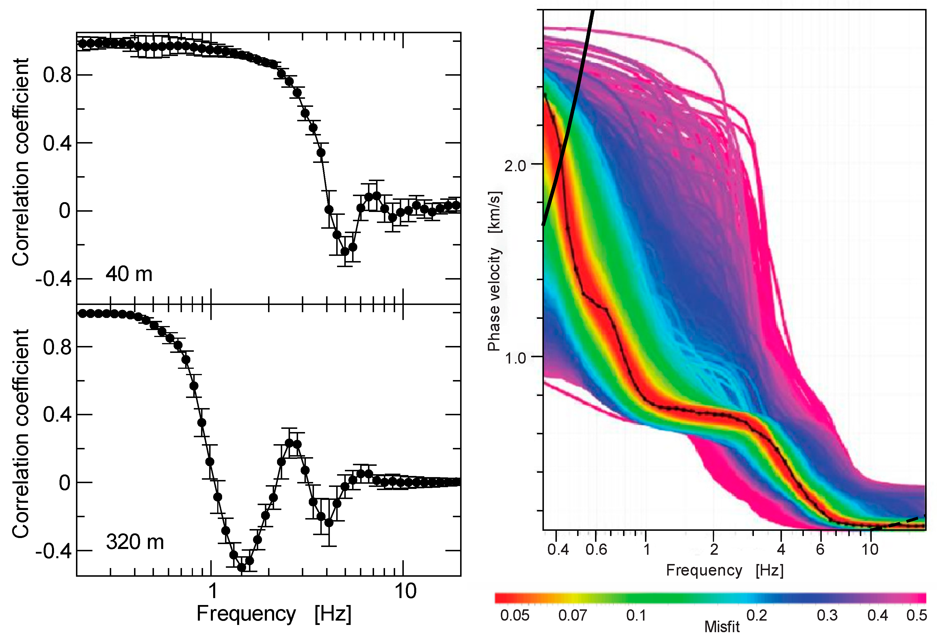
Finally, we consider the results of the SPAC method applied to the ambient noise data recorded by linear arrays of seismographs at the sites, HA and PE (Figure 3). Figure 15 shows two examples of correlation coefficients (K. Aki (1957) [33] used this term to refer to normalized, averaged cross-correlation of seismic noise at a fixed distance; see also [34,35,36]) as a function of frequency. According to the theory of the SPAC method, correlation coefficients should take the form of a Bessel function of first class and order zero. Its argument is frequency times the distance between stations divided by the phase velocity (of Rayleigh waves for the case of cross-correlation of vertical components). The two plots on the left of Figure 15 show correlation coefficients computed for station pairs, separated by distances of 40 and 320 m at the PE site (Figure 3). Our correlation coefficients take the form of a Bessel function, allowing us to estimate the phase velocity of Rayleigh waves as a function of the frequency. The correlation coefficients for the sites, PE and HA, were inverted to estimate phase velocity dispersion curves, which were in turn inverted to obtain shear wave velocity profiles at those sites. The diagram on the right in Figure 15 shows the result for the PE site, computed using GEOPSY [37]. The solid black line shows the phase velocity dispersion curve estimated from all correlation coefficients at site PE. All other lines show the dispersion curves determined from the inversion of the observed phase velocity dispersion using the neighborhood algorithm. The color of each dispersion curve corresponds to the misfit scale shown at the bottom. The thin red band around the observed dispersion curve indicates the inverted dispersion corresponding to the smallest misfit values and is a measure of the uncertainty of the results. Although it is not possible to estimate precisely, a frequency range for which our phase velocity dispersion is a curve is well determined and B. L. N. Kennet (1983) [43] proposed that correlation coefficients are valid in the wavelength range from 2r to 15r, where r is the inter-station distance. The right diagram in Figure 15 shows lines corresponding to 15r for our largest distance (320 m) and 2r for our smallest distance (5 m). We observe that almost all the frequency range shown in Figure 15 may be considered valid according to this criterion.

The final models determined for the two observation sites are given in

Table 2. Shear wave velocity models at PE and HA determined from the SPAC method.

Layer	Thickness (m)	Vs (m/s)	Density (kg/m3)
PE
1	7.5	100	2000
2	17.0	300	2000
Half space	-	800	2000
HA
1	8.0	110	2000
2	19.5	265	2000
Half space	-	765	2000

. A fixed ratio of Vp to Vs of $\sqrt{3}$ was used. We checked that the results did not change assuming Vp/Vs = 2, as argued above. It is well known that phase velocity dispersion curves are not sensitive to Vp values (or, conversely, to Poisson ratio values). These results coincide with the geological information: The topmost layer fits the volcanic ash deposits and the second layer fits the underlying silt and silty clay layer that resulted from the weathering of the underlying pyroclastic flows. The latter would correspond to the halfspace in Table 2. The observed dispersion curve extends to values larger than the 800 m/s chosen to represent the bedrock. We did not invert deeper layers because it becomes difficult to fit the observed dispersion at small frequencies. In addition, although observed phase dispersion suggests that the shear-wave velocity of the bedrock is in excess of 2 km/s, the increase in velocity occurs over a large depth interval and without large impedance contrasts at single interfaces. This is supported by the lack of amplification at small frequencies in our results.

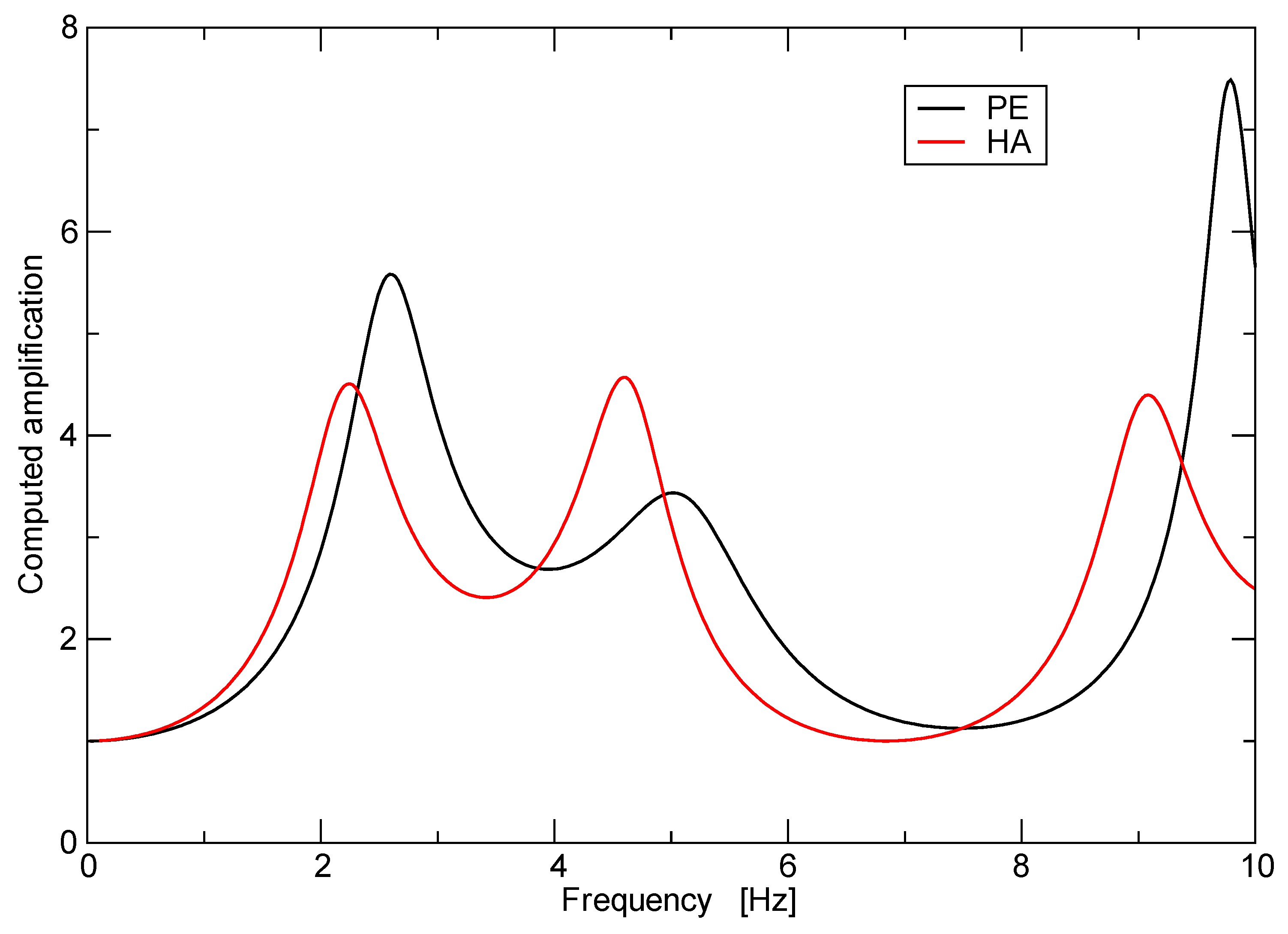
We have used the soil profiles given in Table 2 to compute the expected amplification in Armenia for the vertical incidence of plane shear-waves using the reflectivity method [44]. Figure 16 shows the resulting transfer functions. Lacking data, anelastic attenuation was neglected in this simulation. However, attenuation becomes increasingly significant with increasing frequency, and its effects at the fundamental frequency are minor for reasonable values of the Q factor. Thus, neglecting attenuation has a small effect on our comparisons between observations and modelling, centered on the frequency of the first resonant peak. Figure 16 shows that the maximum amplification is 5.6 for the PE site at 2.6 Hz, and 4.5 for the HA site at 2.3 Hz. The fundamental frequencies coincide with all other estimates, but maximum amplification is underestimated.

5. Discussion

Our study on site effects in Armenia has included previous results and data that were available only in internal reports, as well as new data. Moreover, efforts were made to contrast the different estimates of the site amplification and relate them to available data on the subsoil structure. Thus, for the first time, we may confidently use these results to push for an official seismic microzonation of the city. The use of different data types and different analysis techniques gives us confidence that our amplification estimates are robust, even as amplification values show the usual minimum uncertainty of a factor, 2. Although a seismic microzonation of Armenia is required by law, to date, the lack of an integrated analysis and validation of results has precluded the publication of a microzonation map.

It is not surprising that the site effects in Armenia are significant. The shear wave velocity contrast between the surficial volcanic ash deposits and the underlying pyroclastic flows accounts for computed amplification factors between 4 and 6. This value is slightly smaller than the amplification values estimated from earthquake data, about a factor of 10. We speculate that the value determined for the shear-wave velocity of the bedrock may be underestimated, especially given that the shear-wave velocity values determined for the shallowest layers from the inversion of dispersion curves coincide with the values observed in the seismic cone tests.

Fundamental frequencies vary mainly between 2 Hz and 2.8 Hz (only two points show fundamental frequencies of 1.9 and 1.7 Hz). This is a relatively small range of variation. The shear wave velocity contrast between the surficial deposits and the underlying basement is large enough to render meaningless the variations of shear wave velocity of the topmost layers (between 140 m/s and 250 m/s). In terms of local amplification, it is not worthwhile to differentiate microzones in Armenia, with the available data. Site amplification, which is substantial, varies within the usual minimum uncertainty of a factor of 2. However, because their variations within Armenia are small, our results suggest that site effects are not enough to explain the irregular damage distribution caused by the 1999 event.

We have shown that it is useful to compare different types of data and different techniques of analysis to estimate site effects, even if the results may show some minor discrepancies. For example, the use of response spectral ratios relative to SMSIM simulations of response spectra provide surprisingly good estimates of the observed transfer function, even if average amplification values are underestimated. This is a promising result considering the very little data used to constrain the SMSIM simulations. Moreover, RSR relative to SMSIM provide a better estimate of the amplification than spectral ratios relative to a reference site (SSR). Empirical transfer functions determined using SSR show the same shape as those obtained from earthquake HVSR or RSR, but the amplification is significantly overestimated. We believe that the reason SSR fails to estimate the amplification correctly are unnaturally small amplitudes of earthquake records at our reference station, CAL. Because SSR have the same shape as other estimates, the factor that affects amplitudes at CAL seems to be independent of the frequency. We hypothesize that, because the source locations are close to the recording stations, differences in radiation patterns may decrease significantly the amplitudes of the earthquake recorded at station CAL. Unfortunately, we do not have the data to test this hypothesis. Despite this, our final results show a good agreement between the experimental estimates of site effects and the computed site response, even if computations would be improved by including anelastic attenuation.

We are convinced that the best approach to a microzonation map in Armenia city for the time being, in terms of local amplification, is to consider homogeneous site effects. However, this is in stark contradiction with the observed irregular damage distribution during the 1999 earthquake. This calls for a similarly detailed analysis of the distribution of the vulnerability of the building stock in Armenia. This is the subject of a companion paper that is currently under preparation.

References

1. Monsalve-Jaramillo, H.; Vargas-Jiménez, C.A. El sismo de Armenia, Colombia (Mw = 6.2) del 25 de enero de 1999. Un análisis telesísmico de ondas de cuerpo, observaciones de campo y aspectos sismotectónicos. Rev. Geofís. 2002, 57, 21–57. (In Spanish) [Google Scholar]
2. Sociedad de Ingenieros del Quindío (SIQ). Procesamiento y Análisis de los Formularios de Evaluación de Daños del Sismo del 25 de Enero de 1999 en Armenia (Quindío); Sociedad de Ingenieros del Quindío: Armenia, Colombia, 2002; 63p. (In Spanish) [Google Scholar]
3. Chávez-García, F.J. Site effects due to topography and to soft soil layers: Progress made and pending issues. A personal perspective. In Proceedings of the 5th International Conference of Earthquake Geotechnology Engineering, Santiago, Chile, 10–13 January 2011; pp. 105–136. [Google Scholar]
4. Vargas-Jimenez, C.A.; Monsalve, H.; Bermudez, M.L.; Cuenca, J.C. Utilización de redes neuronales para la determinación de respuestas de sitio a partir de ondas coda: Aplicación para Armenia, Colombia. Earth Sci. Res. J. 2001, 5, 27–31. (In Spanish) [Google Scholar]
5. Parolai, S.; Bindi, D.; Baumbach, M.; Grosser, H.; Milkereit, C.; Karakisa, S.; Zünbül, S. Comparison of different site response estimation techniques using aftershocks of the 1999 Izmit earthquake. Bull. Seismol. Soc. Am. 2004, 94, 1096–1108. [Google Scholar] [CrossRef]
6. Pilz, M.; Parolai, S.; Leyton, F.; Campos, J.; Zschau, J. A comparison of site response techniques using earthquake data and ambient seismic noise analysis in the large urban areas of Santiago de Chile. Geophys. J. Int. 2009, 178, 713–728. [Google Scholar] [CrossRef] [Green Version]
7. Borcherdt, R.D. Effects of local geology on ground motion near San Francisco Bay. Bull. Seismol. Soc. Am. 1970, 60, 29–61. [Google Scholar]
8. Chávez-García, F.J.; Pedotti, G.; Hatzfeld, D.; Bard, P.-Y. An experimental study of site effects near Thessaloniki (Northern Greece). Bull. Seismol. Soc. Am. 1990, 80, 784–806. [Google Scholar]
9. Ktenidou, O.-J.; Chávez-García, F.J.; Pitilakis, K. Variance reduction and signal-to-noise ratio: Reducing uncertainty in spectral ratios. Bull. Seismol. Soc. Am. 2011, 101, 619–634. [Google Scholar] [CrossRef]
10. Lermo, J.; Chávez-García, F.J. Site effect evaluation using spectral ratios with only one station. Bull. Seismol. Soc. Am. 1993, 83, 1574–1594. [Google Scholar]
11. Field, E.H.; Jacob, K.H. A comparison and test of various site-response estimation techniques, including three that are not reference-site dependent. Bull. Seismol. Soc. Am. 1995, 85, 1127–1143. [Google Scholar]
12. Farrugia, J.J.; Atkinson, G.M.; Molnar, S. Validation of 1D earthquake site characterization methods with observed earthquake site amplification in Alberta, Canada. Bull. Seismol. Soc. Am. 2017, 108, 291–308. [Google Scholar] [CrossRef]
13. Castro, R.R.; Mucciarelli, M.; Pacor, F.; Petrungaro, C. S-wave site-response estimates using horizontal-to-vertical spectral ratios. Bull. Seismol. Soc. Am. 1997, 87, 256–260. [Google Scholar]
14. Chávez-García, F.J.; Montalva, G.A. Efectos de sitio para ingenieros geotécnicos, studio del valle de Parkway. Obras y Proyectos 2014, 16, 6–30. (In Spanish) [Google Scholar] [CrossRef]
15. Rosenblueth, E.; Arciniega, A. Response spectral ratios. Earthq. Eng. Struct. Dyn. 1992, 21, 483–492. [Google Scholar] [CrossRef]
16. Khaheshi Banab, K.; Kolaj, M.; Motazedian, D.; Sivathayalan, S.; Hunter, J.A.; Crow, H.L; Pugin, A.J.-M.; Brooks, G.R.; Pyne, M. Seismic site response analysis for Ottawa, Canada: A comprehensive study using measurements and numerical simulations. Bull. Seismol. Soc. Am. 2012, 102, 1976–1993. [Google Scholar] [CrossRef]
17. Hruby, C.E.; Beresnev, I.A. Empirical corrections for basin effects in stochastic ground-motion prediction, based on the Los Angeles basin anslysis. Bull. Seismol. Soc. Am. 2003, 93, 1679–1690. [Google Scholar] [CrossRef]
18. Motazedian, D.; Atkinson, G.M. Stochastic finite-fault modeling based on dynamic corner frequency. Bull. Seismol. Soc. Am. 2005, 95, 995–1010. [Google Scholar] [CrossRef]
19. Atkinson, G.M.; Motazedian, D. Ground-motion amplitudes for earthquakes in Puerto Rico. Bull. Seismol. Soc. Am. 2013, 103, 1846–1859. [Google Scholar] [CrossRef]
20. Boore, D.M.; Atkinson, G.M. Ground-motion prediction equations for the average horizontal component of PGA, PGV, and 5%-damped SA at spectral periods between 0.01 s and 10.0 s. Earthq. Spectra 2008, 24, 99–138. [Google Scholar] [CrossRef]
21. Boore, D.M. Simulation of ground motion using the stochastic method. Pure Appl. Geophys. 2003, 160, 635–676. [Google Scholar] [CrossRef]
22. Konno, K.; Ohmachi, T. Ground-motion characteristics estimated from spectral ratio between horizontal and vertical components of microtremor. Bull. Seismol. Soc. Am. 1998, 88, 228–241. [Google Scholar]
23. Elsner, A.A.; Tsonis, A.A. Singular Spectrum Analysis: A New Tool in Time Series Analysis; Springer US: Berlin, Germany, 1996. [Google Scholar]
24. Carniel, R.; Barazza, F.; Pascolo, P. Improvement of Nakamura technique by singular spectrum analysis. Soil Dyn. Earthq. Eng. 2006, 26, 55–63. [Google Scholar] [CrossRef]
25. Tselentis, G.-A.; Paraskevopoulos, P. Site response analysis of Vartholomio W-Greece from singular spectrum analysis of microtremor and weak motion data. Soil Dyn. Earthq. Eng. 2010, 30, 378–394. [Google Scholar] [CrossRef]
26. Gómez, M. Caracterización de Señales Sísmicas Usando Análisis de Espectros Singulares (SSA) y Transformada de Tiempo Corto de Fourier (STFT). Master’s Thesis, Universidad Tecnológica de Pereira, Pereira, Colombia, March 2016. (In Spanish). [Google Scholar]
27. Nakamura, Y. A method of dynamic characteristics estimation of subsurface using microtremor on the ground surface. QR Railw. Tech. Res. Inst. 1989, 30, 25–33. [Google Scholar]
28. Lermo, J.; Chávez-García, F.J. Are microtremors useful in site response evaluation? Bull. Seismol. Soc. Am. 1994, 84, 1350–1364. [Google Scholar]
29. Arai, H.; Tokimatsu, K. Effects of Rayleigh and Love waves on microtremor H/V spectra. In Proceedings of the 12th World Conference on Earthquake Engineering, Auckland, New Zealand, 30 January–4 February 2000; pp. 2232–2240. [Google Scholar]
30. Mucciarelli, M.; Gallipoli, M.R.; Arcieri, M. The stability of the horizontal-to-vertical spectral ratio of triggered noise and earthquake recordings. Bull. Seismol. Soc. Am. 2003, 93, 1407–1412. [Google Scholar] [CrossRef]
31. Bard, P.Y.; Acerra, C.; Alguacil, G.; Anastasiadis, A.; Atakan, K.; Azzara, R.; Basili, R.; Blarel, F.; Bonnefoy-Claudet, S.; Bordoni, P.; et al. The SESAME Project: An overview and main results. In Proceedings of the 13th World Conference on Earthquake Engineering, Vancouver, BC, Canada, 1–6 August 2004. [Google Scholar]
32. Haghshenas, E.; Bard, P.Y.; Theodulidis, N.P.; Sesame WP04 Team. Empirical evaluation of microtremor H/V spectral ratio. Bull. Earthq. Eng. 2008, 6, 75–108. [Google Scholar] [CrossRef]
33. Aki, K. Space and time spectra of stationary stochastic waves, with special reference to microtremors. Bull. Earthq. Res. Inst. 1957, 25, 415–457. [Google Scholar]
34. Chouet, B.A.; De Luca, G.; Milana, G.; Dawson, P.B.; Martini, M.; Scarpa, R. Shallow velocity structure of Stromboli volcano, Italy, derived from small-aperture array measurements of Strombolian tremor. Bull. Seismol. Soc. Am. 1998, 88, 653–666. [Google Scholar]
35. Chavez-García, F.J.; Rodríguez, M.; Stephenson, W.R. An alternative approach to the SPAC analysis of microtremors: Exploiting stationarity of noise. Bull. Seismol. Soc. Am. 2005, 95, 277–293. [Google Scholar] [CrossRef]
36. Chavez-García, F.J.; Rodríguez, M.; Stephenson, W.R. Subsoil structure using SPAC measurements along a line. Bull. Seismol. Soc. Am. 2006, 96, 729–736. [Google Scholar] [CrossRef]
37. Geopsy. Available online: www.geopsy.org (accessed on 18 June 2018).
38. Lozano, C.; Monsalve, H.; Chávez-García, F. Microtremor analysis to calculate shear waves velocity profiles using the spatial autocorrelation method (SPAC) in Armenia, Colombia. In Proceedings of the VIII Congreso Nacional de Ingeniería Sísmica, Barranquilla, Colombia, 31 May–2 June 2017. [Google Scholar]
39. Boore, D.M. Stochastic simulation of high-frequency ground motions based on seismological models of the radiated spectra. Bull. Seismol. Soc. Am. 1983, 73, 1865–1894. [Google Scholar]
40. SMSIM—Fortran Programs for Simulating Ground Motions from Earthquakes; Version 2.0; a revision of OFR 96-80-A. OFR 00-509; USGS: Menlo Park, CA, USA, 2002.
41. King, J.L.; Tucker, B.E. Observed variations of earthquake motion across a sediment-filled valley. Bull. Seismol. Soc. Am. 1984, 74, 137–151. [Google Scholar]
42. Jarpe, S.P.; Cramer, C.H.; Tucker, B.E.; Shakal, A.F. A comparison of observations of ground response to weak and strong ground motion at Coalinga, California. Bull. Seismol. Soc. Am. 1988, 78, 421–435. [Google Scholar]
43. Henstridge, J.D. A signal processing method for circular array. Geophysics 1979, 44, 179–184. [Google Scholar] [CrossRef]
44. Kennett, B.L.N. Seismic Wave Propagation in Stratified Media; Cambridge University Press: Cambridge, UK, 1983; ISBN 0521239338. [Google Scholar]
Figure 1. Upper left: Location of Armenia in Colombia, South America. The rectangle indicates the area plotted in the main figure. The main figure shows the geological map of the region around the city of Armenia (the white irregular shape indicates the extension of the city). The main rivers are shown as a reference. Geological formations include volcanic, sedimentary, and metamorphic rocks. Black stars indicate the location of towns around Armenia. The line, AA’, indicates the location of the geological cross-section shown in Figure 2. The solid rectangle indicates the area plotted in Figure 3.
Geosciences 08 00254 g001
Figure 2. Geological cross-section of Armenia along the line marked AA’ in Figure 1. The thick red lines indicate normal faults.
Geosciences 08 00254 g002
Figure 3. Location of the epicenter of the main shock of the 1999 earthquake (star) and of the nine analyzed aftershocks (solid circles, the numbers refer to Table 1). The contour with thick solid line indicates the city of Armenia. Triangles indicate the location of the accelerograph stations that recorded the aftershocks. Two squares indicate the two locations (HA and PE) where linear seismograph arrays were used to record microtremors, analyzed using the spatial autocorrelation (SPAC) method. Open circles indicate the location of towns around Armenia.
Geosciences 08 00254 g003
Figure 4. Example of the acceleration records of the aftershocks (frames on the left) and their Fourier amplitude spectra (frames on the right). The traces shown correspond to event 7 (Table 1), recorded by stations, CAL and UNI. Spectra plotted with black lines correspond to station CAL, while those plotted using red lines correspond to station UNI.
Geosciences 08 00254 g004
Figure 5. Site amplification at station EST determined from aftershock analysis. The two upper diagrams show the results of spectral ratios relative to a reference site (SSR) technique (CAL is the reference station) for the two horizontal components. The two bottom diagrams show the corresponding result using the horizontal relative to the vertical component (HVSR) technique.
Geosciences 08 00254 g005
Figure 6. Average site effects estimated for station EST using earthquake data and ambient noise records. Earthquake data was analyzed using SSR and HVSR. Seismic noise was recorded using a seismograph (HVSR noise seism.) and an accelerograph (HVSR noise accel.). The two diagrams correspond to the two horizontal components.
Geosciences 08 00254 g006
Figure 7. Average spectral amplitudes for the three components of ground motion (horizontal motion EW and NS; VR stands for vertical) computed for the broad band records of seismic noise at station EST. Solid lines indicate average values. Dashed lines show average values plus or minus one standard deviation. A total of 236 amplitude spectra, each one corresponding to a 60-s duration window of ambient noise, were averaged for each component.
Geosciences 08 00254 g007
Figure 8. Site amplification estimated at the reference station, CAL. We show average HVSR results computed using earthquake data and ambient noise recorded using a seismograph and an accelerograph. The two diagrams correspond to the two horizontal components.
Geosciences 08 00254 g008
Figure 9. Estimates of site response for station EST calculated as response spectral ratios (RSR) of aftershock records. Each line corresponds to one event. Black lines show the results of RSR relative to station CAL. Red lines show the estimates obtained using response spectra computed using SMSIM as reference. Each frame corresponds to one component, EW, NS, and vertical.
Geosciences 08 00254 g009
Figure 10. Triangles: Fundamental frequency for the vertical component at the five sites where aftershocks were recorded, obtained from the different methods used to estimate site response. The boxes show the average fundamental frequency for the two horizontal components: The limits of the box show the lower and upper quartiles, the whiskers indicate the lower and upper extreme values, and the line inside the box indicates the median value.
Geosciences 08 00254 g010
Figure 11. Horizontal amplification at each of the five sites where aftershocks were recorded, obtained from the different methods used to estimate site response. The limits of the box show the lower and upper quartiles, the whiskers indicate the lower and upper extreme values, and the line inside the box indicates the median value.
Geosciences 08 00254 g011
Figure 12. Amplification estimated at sites, CAR and EST, from HVSR computed for ambient noise data. We compare the results using ambient noise recorded using an accelerograph (hvsr noise accel.) and a broad band seismograph (HVSR noise seism.) in August 2017, with the results from measurements made in 2002 (HVSR noise 2002). Results for CAR are compared with 2002 data, recorded at a point 87 m away, to the NE. Results for EST are compared, with a point 582 m away, to the SW.
Geosciences 08 00254 g012
Figure 13. Spatial distribution of the fundamental frequency in Hz (red lines). The black line shows the city of Armenia. Red circles show locations of ambient noise measurements in 2002 together with their fundamental frequency value. Solid triangles show the stations that recorded aftershocks of the 1999 event. Green symbols mark seismic cone measurements, with their average shear wave velocity.
Geosciences 08 00254 g013
Figure 14. Spatial distribution of the horizontal amplification (red lines). The black line shows the city of Armenia. Red circles show locations of ambient noise measurements in 2002 together with their amplification value. Solid triangles show the stations that recorded aftershocks of the 1999 event. Green symbols mark seismic cone measurements, with their average shear wave velocity.
Geosciences 08 00254 g014
Figure 15. Panels on the left: Two examples of correlation coefficients computed from average cross-correlation of vertical component ambient noise records obtained using the linear array deployed at PE (Figure 2). Each frame shows the average values for two stations. The distance between them is indicated. Fitting a Bessel function of first kind and zero order to these curves allows us to estimate the phase velocity dispersion curve of Rayleigh waves at the site. Right panel: Final observed dispersion curve at PE (solid black line) together with the dispersion curves inverted using [37]. Each computed dispersion curve is color coded to the misfit shown at the bottom. The thick solid in the upper left corner indicates wavelengths equal to 15 times 320 m. The thick dashed line in the bottom right corner indicates wavelengths equal to 2 times 5 m.
Geosciences 08 00254 g015
Figure 16. Transfer functions computed for the vertical incidence of shear waves on the soil profiles derived from the SPAC method at the sites, PE and HA, shown in Table 2. Lacking data, anelastic attenuation was neglected in this simulation.
Geosciences 08 00254 g016