A Site Amplification Model for Crustal Earthquakes

Civil Engineering Department, Hacettepe University, Ankara 06800, Turkey
*
Author to whom correspondence should be addressed.
Geosciences 2018, 8(7), 264; https://doi.org/10.3390/geosciences8070264
Submission received: 19 February 2018
/
Revised: 21 June 2018
/
Accepted: 12 July 2018
/
Published: 17 July 2018
(This article belongs to the Special Issue Site-Specific Seismic Hazard Analysis: New Perspectives, Open Issues and Challenges)
Abstract
:A global dataset which is composed of more than 20,000 records is used to develop an empirical nonlinear soil amplification model for crustal earthquakes. The model also includes the deep soil effect. The soil nonlinearity is formulated in terms of input rock motion and soil stiffness. The input rock motion is defined by the pseudo-spectral acceleration at rock site condition (PSArock) which is also modified with between-event residual. Application of PSArock simplifies the usage of the site model by diminishing the need of using the period-dependent correlation coefficients in hazard studies. The soil stiffness is expressed by a Gompertz sigmoid function which restricts the nonlinear effects at both of the very soft soil sites and very stiff soil sites. In order to surpass the effect of low magnitude and long-distant recordings on soil nonlinearity, the nonlinear site coefficients are constrained by using a limited dataset. The coefficients of linear site scaling and deep soil effect are obtained with the full database. The period average of site-variability is found to be 0.43. The sigma decreases with decreasing the soil stiffness or increasing input rock motion. After employing residual analysis, the region-dependent correction coefficients for linear site scaling are also obtained.
1. Introduction
The site amplification is defined as the ratio of ground-motion intensity measure (GMIM) at a site to the motion observed at reference rock-site condition [1]. One of the efficient procedures to compute site amplification is the application of the non-reference site amplification method [2]. In this method (e.g., [2,3,4,5,6,7]), ground-motion prediction equations (GMPEs) can be used to predict the ground-motion at reference rock-site condition and then normalize the empirically available GMIM to obtain site amplification.
Generally speaking, the current site amplification models impose three important soil behavior. The first one is the linear site response which is currently modeled with a continuous function of VS30 (time-based average of shear wave velocity of top 30 m soil media) after Boore et al. [8]. The site amplification is assumed to decrease linearly with increasing natural logarithm of VS30 [6,7,8,9,10,11,12,13]. Some researchers uses a period-independent fixed reference VS30 for linear scaling (e.g., 760 m/s in [12]) or period-dependent reference VS30 (e.g., [13]). Using either period-independent or dependent values does not affect the slope of linear site scaling [14]. Due to the low number of recordings at high VS30 sites, a constant amplification portion at the high VS30 values is preferred. Some model developers use period-dependent limiting VS30. At short periods, it reaches 1500 m/s and at longer periods, this value decreases to 400 m/s [15,16,17]. The period independent constraining value can be used as well (e.g., VS30 = 1000 m/s in [7] or 1130 m/s in [18]). The second behavior in site amplification is soil nonlinearity, which is again modeled using VS30, which represents soil stiffness and input rock motion [6,7,9,10,11,12,13,15,16,17,18,19,20,21]. The level of soil nonlinearity decreases as soil stiffness increases or input rock motion decreases. The final behavior is the deep soil effect which is modeled with the depth to rock parameter (e.g., Z1, depth to VS profile reaches 1 km/s [21]).
Another important site parameter is the fundamental site frequency, f0 (e.g., [22,23]). Although the results might be changed for global data, for European data, Sandıkkaya and Akkar [24] show that the use of the VS30-f0 pair in site scaling leads a slight decrease the within-event sigma when it is compared with the VS30-Z1 pair. As well, none of the reference databases (see next section) provides f0. Consequently, within the context of this study we cannot use f0 as a site parameter.
There are two functional forms, which are discussed in the context of this study, to describe the soil nonlinearity. Zhoa et al. study [15] also proposed a functional form but it employs a predominant site period, so that it will not be elaborately discussed. The discussions related to previously published site models (e.g., [6,9,10,11,20]) can be found in detail in the Sandıkkaya et al. [7] study. The first functional form, proposed by Walling et al. [11], is generated by employing ground motion simulations and site response analysis. Sandıkkaya et al. [7] site model uses this functional form but computes the nonlinear coefficients with empirical data. Later, Kamai et al. [13] modified the Walling et al. study with an increasing number of simulations and site response analysis. The soil nonlinearity is formulated as a multiplication of the nonlinear site coefficient with a function including both input rock motion and soil stiffness. Chiou and Youngs [10] offered the second functional form which is also used by Seyhan and Steward [12] (SS14 or BSSA14, Boore et al. [17]—throughout the text we use them interchangeably but they refer the same site model) and Chiou and Youngs [19] (CY14). Contrary to the Walling et al. model, to compute the soil nonlinearity, the nonlinear site coefficient is multiplied with two functions: one including input rock motion and the other including VS30. Application of the second functional form seems more practical, especially in computing the variability of site amplification in terms of either VS30 or input rock motion or both.
In this study, we consider linear and nonlinear site behaviors together with deep soil effect to simulate site amplification. In the following sections, we firstly give details about the strong-motion database that we use in the regressions. Secondly, a rock motion GMPE is generated to estimate the ground motion intensities at reference rock site condition. Thirdly, site amplification ratios are computed and the regressions are performed to obtain site model coefficients. Then, the site variability is expressed in terms of PSArock and VS30. The paper continues with a comparison of the proposed model with some of the site models in the literature. Finally, we employ residual analysis to investigate the possible regional effects in the linear site response term.
2. Ground-Motion Database
A global strong-motion dataset is merged from the global NGA-West2 dataset [25], regional European datasets [26,27], and local Iran, Japanese and Turkish datasets [28,29,30]. The NGA-West2 database is composed of only five earthquakes from Japan (1925 records) and 119 earthquakes from Europe and the Middle East (524 records). Thus, the data from Europe, the Middle East and Japan in the NGA-West2 database was enhanced by local and regional databases. The database consists of stations with measured VS30 and accelerograms recorded within 300 km (Joyner-Boore distance, RJB is used). The lower moment magnitude (Mw) limit of normal, reverse, and strike-slip earthquakes was 3.5. Only shallow crustal earthquakes with a maximum depth of 35 km are used. Finally, we used only events and stations with at least two recordings (only exceptions are made to Mw + 6.75 events recorded at soft sites with VS30 < 360 m/s, due to not losing any possible nonlinear site effects). Generally, in single-station sigma studies (e.g., [31]), at least 10 recordings per station was used. We cannot follow such criterion because if it were applied, most of the stations would be removed, as well as we would lose some records that might have possible nonlinear site effects.
We use eight larger seismic regions by following Flinn et al. [32]. The regions are listed in Table 1. Since there are only three events from Alaska and New Zealand regions, they are merged with earthquakes occurred in “Oregon, California and Nevada” region. Guam to Japan, Japan–Kuril Islands–Kamchatka Peninsula, Southwestern Japan and Ryukyu Islands, and Eastern Asia regions were labelled as Japan in the context of this study. The waveforms from western Caucasus and Armenia and Northern Italy were considered as western Asia and western Mediterranean areas, respectively.
The database is composed of 20,070 waveforms from 1378 earthquakes recorded at 2134 stations. The seismological features of the database are presented in Figure 1. The Mw-RJB distribution of the database is shown in Figure 1a for larger seismic regions used in this study. The database is dominated by low-magnitude and long-distant records. The distribution becomes sparse as the magnitude increases and distance decreases. The effect of the low number of such recordings on nonlinear site effects is discussed in the following section. Figure 1b shows the depth distribution of normal, reverse, and strike-slip earthquakes. Almost all types of earthquakes were well distributed for depths less than 15 km. This database also overcomes the drawbacks of NGA-West2 and RESORCE databases, which have a sufficiently low number of normal and reverse earthquakes, respectively. Figure 1c shows the distribution of PSA at T = 0.01 s versus VS30 of the database. The data was well sampled for stiff sites. The distribution loosened both in rock and very soft sites.
The geometric average of the two horizontal components was used. It is noted that, the NGA-West2 database gave orientation-independent spectral coordinates. For the waveforms provided in the PEER Strong Motion Database (peer.berkeley.edu.tr; last accessed: 17 October 2017), we computed the geometric average of the horizontal components. For the restricted waveforms, we apply period-dependent correction factors provided by Figure 4 of [33] to compute geometric average of waveforms from the given orientation-independent spectral ordinates. The period range of this study was limited to 4 s since we observed no significant nonlinearity beyond this period, as well as the number of records being decreased due to a usable period range (especially for the European data).
3. Ground Motion Prediction Equation for Rock Motion
A predictive model for GMIM at reference rock site condition which is represented by VS30 = 760 m/s was generated to compute site amplification values. The functional form used to compute the median natural logarithm of pseudo-spectral acceleration at 5% damping ratio, ln(PSArock) was composed of event scaling (magnitude scaling and style-of-faulting, SoF terms), distance scaling (geometric and anelastic attenuation terms), and site scaling (linear site response term) (Equations (1)–(7)). The regression coefficients and between-event residuals (ηi), between-site residuals (δj) and within-event residuals (εij) were computed with the random-effects algorithm proposed by Bates et al. [34]. These residuals were assumed to have normal distributions with standard deviations of σe, σs and σw with the total variability of σt [35].
We used a quadratic magnitude scaling with a break in the linear slope. The hinged magnitude that differentiates low-to-moderate and high-magnitude behavior was chosen as 6.75 by visual inspection of between-event residuals of events whose magnitudes were greater than 6.5. This magnitude scaling is also used in [21,36]. FN and FR are dummies to represent the style-of-faulting effects of normal and reverse events with respect to strike-slip events, respectively. The Joyner-Boore distance metric, RJB was used in the regressions to surpass the hanging-wall effect as in Boore and Atkinson [9] predictive model. Both anelastic and geometric attenuation terms were included in distance scaling. The geometric attenuation term is magnitude dependent. The fictitious depth term, R0, was taken constant (10 km) in the regressions. The linear site response term with VS30 was employed and the site amplification for high VS30 values (1000 m/s) was constrained.
The regional effects were also included in the regressions to predict reference rock site estimates. After computing the regression coefficients for the global model, we inspected the between-event, between-site, and within-event residual distributions. For each region, we added a region-dependent constant to fix the biases observed in event and site terms. In distance scaling, the records from China, western Asia (e.g., Iran), and western Mediterranean (e.g., Italy) had biased estimates with the global model. They were removed by adding region-dependent anelastic attenuation constants. This was parallel to findings of NGA-West2 GMPEs [16,17,18,19]. However, we did not observe any trend in waveforms from Japan. One of the possible explanation could be that our database was dominated by records from this region.
The residual analysis for each independent variables was then performed. Figure 2 displays the between-event (top row) and within-event (bottom row) residual distributions for magnitude- and distance-scaling at T = 0.2 s (left panel) and T = 1 s (right panel), respectively. No major trends (or negligible trends) in these plots indicated that the performance of the GMPE was quite satisfactory. Although in short distances (RJB < 20 km) the median estimations tended to be underestimated, at this stage of the study we did not apply any near-field correction. The between-site residuals were not shown in these plots, because they were very similar to the distribution observed in Figure 9 (please see the section entitled “Regional Effects”).
4. Site Amplification Model
Initial attempts to compute the nonlinear site coefficients showed that they were sensitive to the database limits. The slope of linear site response increases when the database that was abundant in terms of low magnitude events or long-distant records was used. This yielded lower nonlinear coefficients (impose high nonlinearity) to capture the nonlinear site effects existing in the data. Thus, a two-step regression was applied to compute the model coefficients. At the first stage, the period-dependent site model coefficients were computed with a sub-database which was composed of only moderate to strong magnitude events (Mw > 4.5) recorded within 80 km. At the second stage (the full database is used), the nonlinear site coefficients were constrained from the first stage analysis; then the linear and deep soil coefficients were computed. A similar approach was also used in SS14.
Before presenting the proposed site model, the functional form given in SS14 (Equation (8)) was applied to the current study, and the findings were discussed. The model coefficients were γ1, γ2 and γ3. The soil nonlinearity was computed with the multiplication of nonlinear site coefficient, γ1 with the input rock motion term and soil stiffness term. In order to represent the seismic demand on rock, SS14 preferred peak ground acceleration at the rock site (PGArock) as an input parameter. They also fixed the γ2 coefficient to 0.1 g, to fulfill a smooth transition in input rock-motion levels. The soil stiffness was expressed by an exponential function in terms of VS30. This term is decreasing with increasing VS30 and for rock sites (VS30 > 760 m/s) it becomes zero. The γ3 coefficient was adapted from CY14 site model.
We compared the linear and nonlinear site coefficients of Alternative I, which was computed by applying Equation (8) with PSArock at 0.01 s (by assuming PGArock is equal to PSArock at 0.01 s) to Alternative II which considers PSArock at 0.01 s and between-event residuals. The linear site coefficients with two alternatives were comparable (Figure 3a). The SS14 model had lower coefficients than both alternatives resulting in higher amplification. Alternative I yielded similar nonlinear coefficients with the SS14 model at the short-period range (0.1–0.5 s) where strong nonlinearity is observed (Figure 3b). However, the Alternative II that considers between-event residuals, imposed lesser soil nonlinearity in this interval period. The results from the Alternative II were more reliable. When employing non-reference site amplification method, the median estimate for rock motion from a GMPE could be overestimated or underestimated. Thus, this bias should be removed [19]. Since the influence of soil nonlinearity diminishes at longer periods, all coefficients were similar.
We then compared the use of PSArock at 0.01 s and PSArock (between-event residuals are taken into account) in the regressions, and negligible differences were observed in median site amplification estimates. Besides, the choice did not affect the site variability. This was parallel to findings of Sandıkkaya et al. [7] and Kamai et al. [13]. We preferred to continue with PSArock because it diminished the need to correlation coefficients between the period of interest and PSArock. This simplifies applications in the hazard analysis.
The soil stiffness term (VS30-dependence) of the nonlinear functional form in SS14 site model linearly decreased with increasing logarithm of VS30 for soft sites having VS30 < ~350 m/s where nonlinearity was more pronounceable (Figure 3c). Instead of this formulation, we preferred to use a Gompertz sigmoid function. This function scales the soil nonlinearity linearly within a range of 200–400 m/s. This function is also capable of capping the rate of increase below 200 m/s. This enabled us to remove unwanted bias in very soft sites where the number of stations (or recordings) is limited.
In the proposed soil model, the natural logarithm of site amplification, ln(Amp) consists of linear site scaling, deep soil effect, and soil nonlinearity (Equation (9)). The reference rock site condition is selected as VS30 = 760 m/s and the site amplification was constrained for rock sites having VS30 > 1000 m/s. The Z1 scaling of the proposed model was different from SS14 and CY14 site models. The deep soil effect was not considered in SS14 for periods shorter than 0.65 s. This period was 0.25 s in CY14 site model. In both models, the difference between measured and estimated Z1 values was used. However, Rodriguez-Marek et al. [30] study, which uses Z0.8 (depth at which shear-wave velocity attains 800 m/s), gives coefficients for shorter periods. The deep soil effect in the proposed model expressed in terms of the natural logarithm of the Z1 in meters. Since the number of stations with measured Z1 values is quite limited in the database, for the stations with unknown Z1 values, we employed VS30 − Z1 relations given by CY14. Using estimated Z1 values in the regression did not cause any increase in between-site sigma. The period-independent b4 and b5 values were tuned before regression analysis to diminish the soil stiffness effect in high VS30 values and constrain the soil nonlinearity at very soft sites.
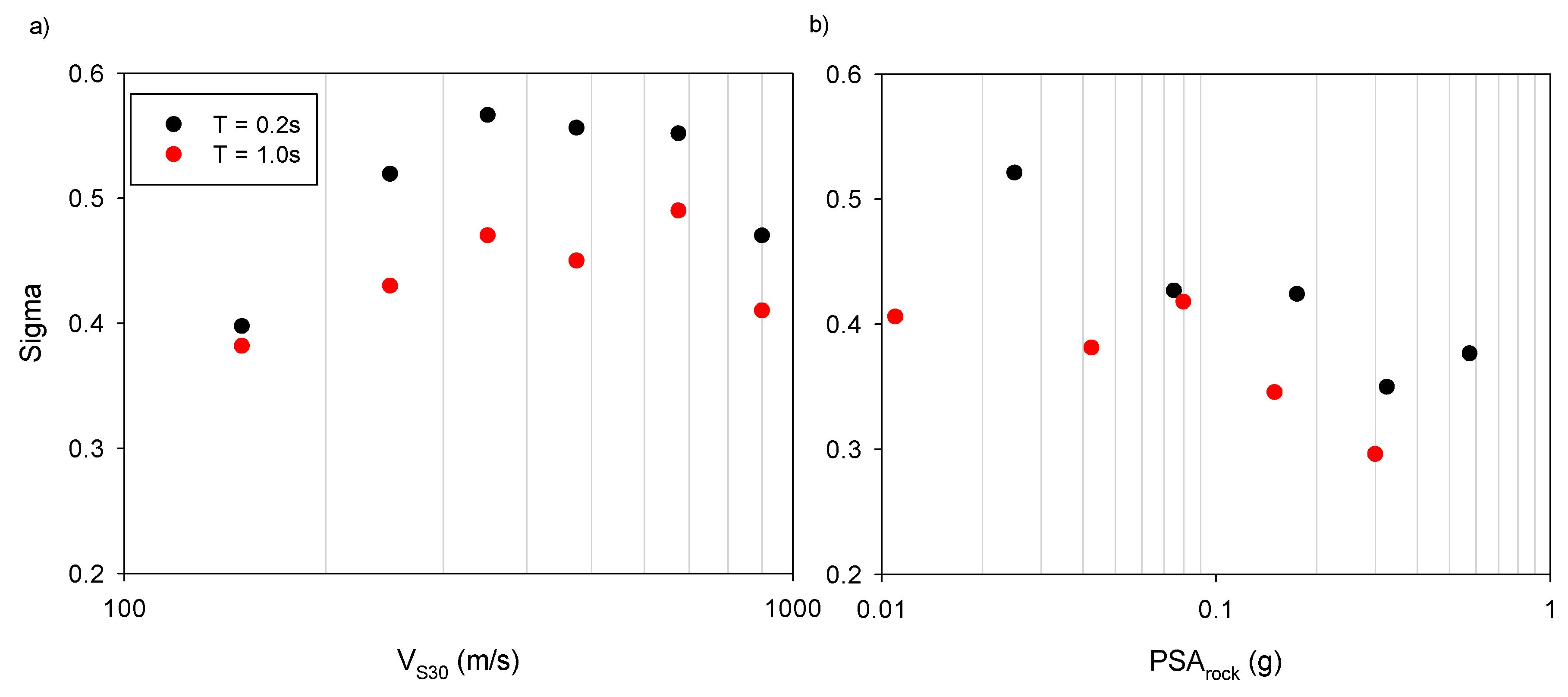
The period-dependent standard deviation of between-site residuals, σs was found between 0.34 and 0.51. It was noted that this sigma value was obtained with the assumption of a homoscedastic model. This assumption was removed and how the variability of site amplification changes with VS30 and PSArock bins was investigated for T = 0.2 s and 1 s (Figure 4). The sites were grouped as very soft sites (VS30 ≤ 200 m/s), soft sites (200 < VS30 ≤ 300 m/s), stiff sites (300 < VS30 ≤ 400 m/s), moderate stiff sites (400 < VS30 ≤ 550 m/s), very stiff sites (550 < VS30 ≤ 800 m/s), and rock sites (VS30 > 800 m/s). We used PSArock bins to classify very weak motion, weak motion, moderate motion, strong motion, and very strong motion (please read the caption of Figure 4 for PSArock bins).
At T = 0.2 s, the site-variability was the largest at very stiff sites. At T = 1.0 s, a similar trend was also observed. However, for rock sites, at both periods, variability was lower than very stiff sites. When compared to number of records at very stiff sites with those at rock sites, the first group had the larger number of records. This might be a reason for decreasing the sigma. The variability decreased from stiff sites to very soft sites. We should cap the variability at very soft sites because the rate of decrease might result in a very low standard deviation. As PSArock increases, the variability decreased, which is common in practice. Similar capping can also be made for lower and upper bounds of PSArock values. The VS30 and PSArock dependent site variability is given in (Equations (10)–(12)).
where c0 is the site variability constant and c1 and c2 represent the slope of PSArock and VS30 terms, respectively. The coefficients for the site model and standard deviation model are given in Table 2.
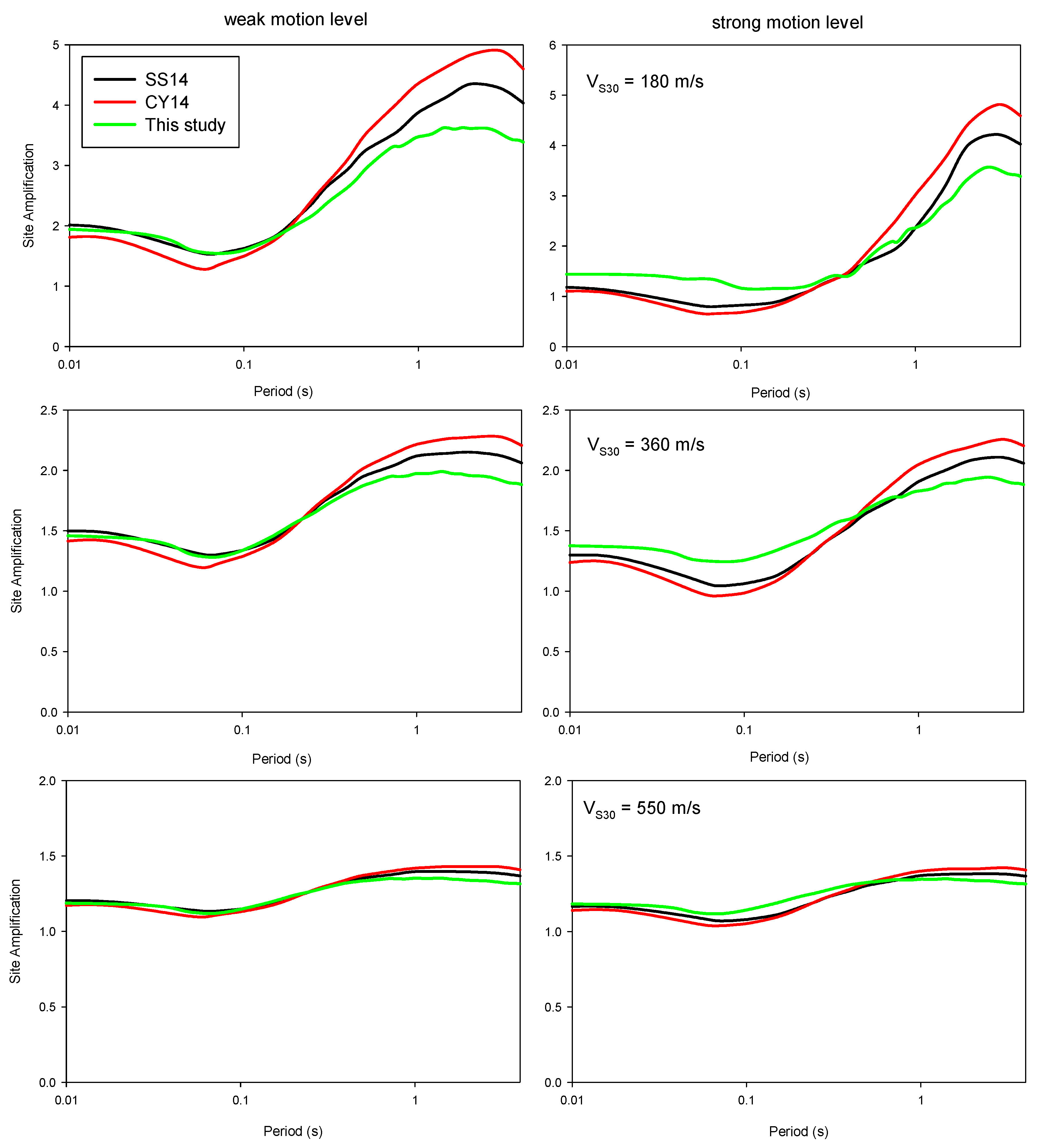
The proposed site model is compared with the SS14 and CY14 site models. The nonlinear soil behavior of the proposed model is dominant at short periods and gradually diminishes after 1 s, and almost vanishes after 2.5 s. We did not observe any nonlinearity after 3 s. This was parallel to findings of SS14 and CY14 (e.g., SS14 had some nonlinearity after 3 s but their nonlinear coefficients were approximately zero).
Figure 5 shows the period dependency of site amplification estimations at VS30 = 180 m/s (very soft soil), VS30 = 360 m/s (stiff soil) and VS30 = 550 m/s (very stiff soil) for weak and strong input rock motion levels. At weak motion levels, our estimations were lower than estimates of the SS14 and CY14 site models, on the other hand, as input rock motion level increased due to the lower nonlinearity imposed in our model, our estimations became higher than SS14 and CY14 site models at short periods. Generally, the proposed model produced lower amplifications at long periods. The amplification estimations were very close to the SS14 and CY14 site models at very stiff sites. As sites get softer, the difference in amplification becomes more visible in this period interval. The observed differences are due to modeling approaches and database features (especially including more data from Japan) in the regressions.
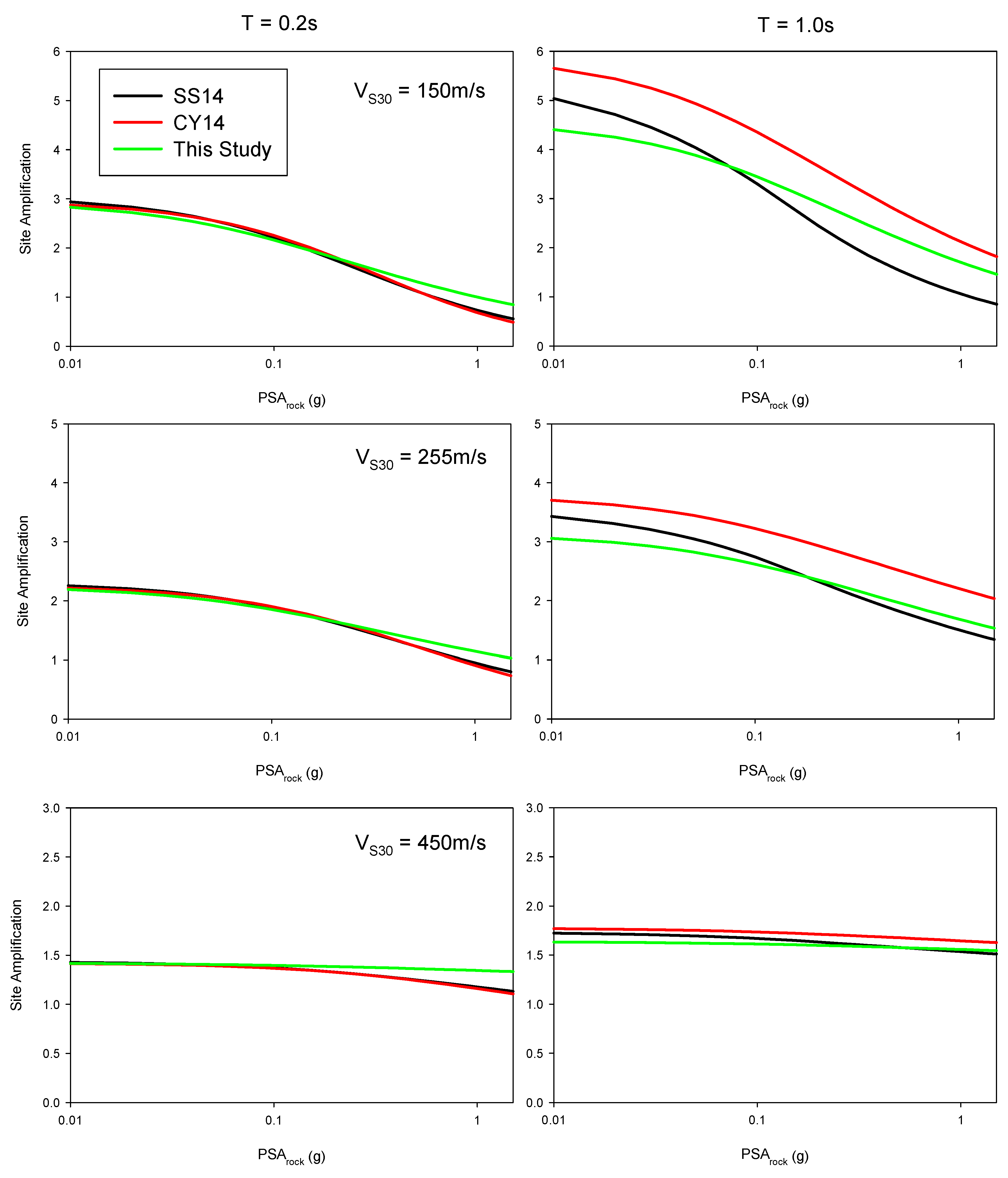
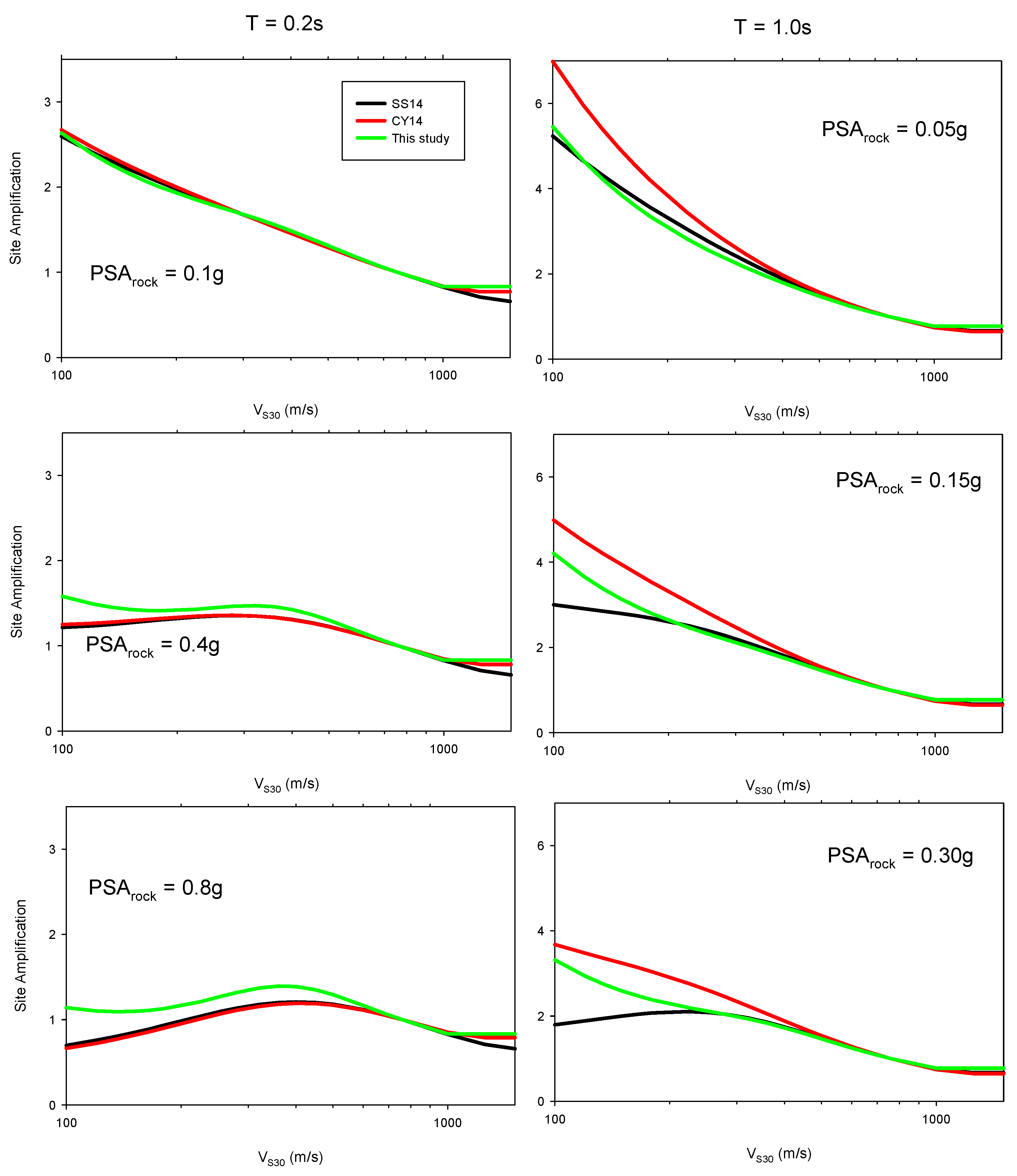
Figure 6 and Figure 7 compare the PSArock and VS30 dependence of site amplification at 0.2 s (right column) and 1.0 s (left column), respectively. In Figure 6, three site conditions (VS30 = 150 m/s, 255 m/s and 450 m/s) were considered. We selected weak, moderate and strong PSArock for the comparisons in Figure 7 (read the figure caption for the PSArock values). At T = 0.2 s, the site amplification estimations of the proposed model matched with the SS14 and CY14 site models at low seismic demands. As PSArock increases, our model tended to estimate lower amplification demonstrating less soil nonlinear behavior. At VS30 = 450 m/s, although CY14 and SS14 models had some nonlinearity, the proposed model was not very sensitive to PSArock. At T = 1 s, for stiff sites, amplifications were generally lower than the CY14 site model. Due to the lower nonlinear site behavior of our model, as PSArock increased, the amplification became higher when compared to the SS14 site model. For the VS30-scaling of the proposed model, SS14 and CY14 site models were similar at stiff site condition. However, as VS30 decreased the differences became more prominent. The 1 s amplification was matched with the SS14 site model, with both models producing lower amplification when compared to the CY14 site model.
5. Regional Effects
Within the context of this study, it was assumed that the nonlinear site and deep basin effects are region-independent. That is, if an amplification trend from one region is different from another, it is because of linear site response. The average of between-site residuals for each region were less than 1% because of application of region-dependent constants in the rock GMPE, and these biases are found to be statistically insignificant. Yet, this analysis did not provide any information about regional VS30 scaling. To do so, we added a region-dependent correction factor, ck, to the linear site term (Equation (13)).
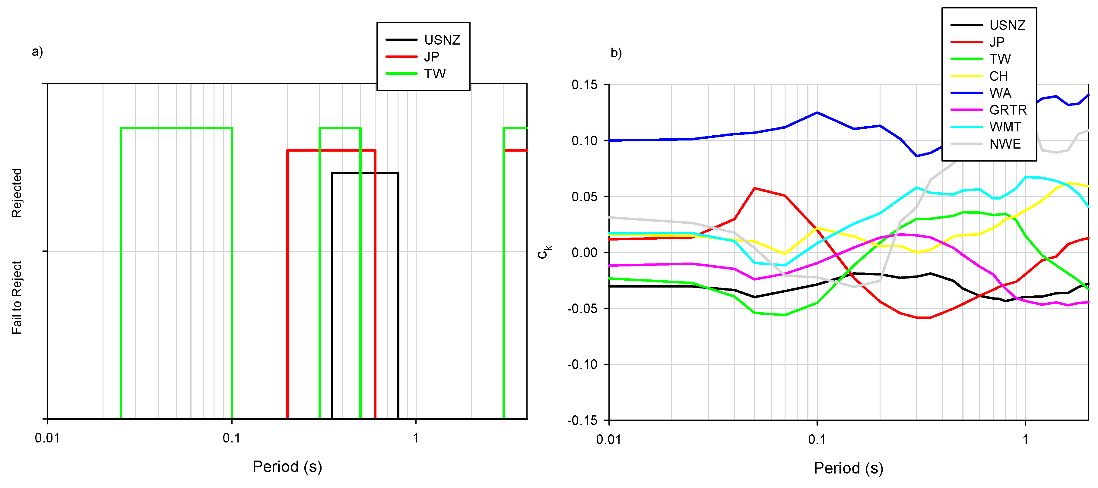
We applied a significance level of 0.05 to test to the ck values to determine whether the regional site amplification scaling was similar to the global site amplification trend or not. That is, the hypothesis ck was equal to zero is tested for each region. Figure 8a shows the test results. The site amplification trend for CH (the acronyms for each region is given in Table 1) was found to be statistically insignificant whereas the hypothesis is rejected for WA in all period range. At only one or two periods, the slopes were found to be statistically significant for GRTR, WMT and NWE regions. These results for these regions were thus not given in Figure 8a. For periods lower than 0.1 s, the test results for region-dependent VS30-scaling of TW sites indicated that different slopes to the global model should be used. At periods of 3 s to 4 s, both TW and JP had significant different slopes. At short periods (0.2–0.8 s), TW, JP, and USNZ slopes were found to be statistically significant. We give all ck values in Table 3 but the statistically significant ones are highlighted with bold font. The period variation of the correction factor is shown in Figure 8b.
Figure 9 shows regionally corrected between-site residuals at T = 0.2 s (left panel) and T = 1.0 s (right panel) for each region (from top to bottom: USNZ, JP, TW, CH, WA, GRTR, WMT, and NWE). The between-site residuals were almost uniformly distributed. We classified the stations as very soft, soft, stiff, very stiff, and rock sites. The average of between-sites residuals of each group is also shown with its standard deviation in these plots. The very soft and rock sites from JP and WMT were underestimated at T = 0.2 s. Due to the low number of stations in some bins (e.g., WA very soft sites, TW stiff sites and CH very stiff sites at T = 1 s), biases were observed. Nevertheless, for each region, the residuals generally show no major trend.
The variability of site amplification (computed by observed PSA value divided by estimated PSArock and between-event residuals) for each region is plotted for VS30 (left panel) and PSArock (right panel) bins for T = 0.2 s (top row) and T = 1.0 s (bottom row) in Figure 10. The intervals of VS30 and PSArock are given in the figure caption. The regional variability also had a wide range for both VS30 and PSArock bins. For example, soft-soil site standard deviation was 0.2 and 0.55 for the TW region and JP region, respectively. Rock-site standard deviation was generally lower than very stiff site sigma. There is a decreasing trend from very stiff sites to very soft sites. However, for some regions this observation did not hold, with larger variability being computed at very soft sites. The similar observation for PSArock could also be made. The fact that the site bins did not have uniform station distribution, and also an unbalanced number of recordings (besides not uniform magnitude distance scatters) for each region, were the main reasons for violating the general observation.
6. Conclusions
In this study, we propose a new nonlinear site amplification model that also considers the deep soil effect. A global database composed of records from western United States, Japan, Taiwan, China, New Zealand, Iran, Turkey, Greece, Italy, Switzerland, and France is used to compute site model coefficients. The functional form of the proposed site model is adopted from SS14 and CY14 site models. The proposed model makes use of soil stiffness and level of input rock motion to describe the soil nonlinear behavior. We refine the exponential functional form to define soil stiffness with a Gompertz function that restricts the nonlinear behavior at low-velocity sites. The agreement between the site amplification estimations with the SS14 and CY14 models and the unbiased residual distributions advocate the reliability of the proposed site model. The variability of the site model is expressed in terms of VS30 and PSArock. As sites get softer or PSArock increases, the variability of the site amplification decreases. This study also focused on the regional differences in site effects. Regional differences are found to be statistically insignificant for CH, GRTR, WMT, and NWE. However, the site amplification observed in WA, USNZ, JP, and TW are different from the global VS30-scaling.
The soil nonlinearity is found to be lower than previous site models. One of the possible reasons is that we use a large database but the number of records with nonlinear site effects is limited. Besides, using a lower number of records per station resulted in a higher sigma than previous studies. These drawbacks can be solved by merging the features of the empirically derived site models with simulation-based site amplification studies (e.g., Kamai et al. [13]).
It is recommended that the applicability the model extends to 150 < VS30 < 1200 m/s. The proposed site model can be served as a site-scaling term in the future ground motion prediction equations. We also emphasize that when it is the case, only nonlinear site coefficients should be used and the coefficients for linear site response and deep soil effects should be computed in the regression steps. The site model can also be considered as a candidate site model in the computation of the regional site factors for seismic design codes (e.g., [37]).
Author Contributions
This study is a part of L.D.D’s MS thesis.
Funding
This study is funded by The Scientific and Technical Research Council of Turkey (TUBITAK) under Project No: 117M146.
Acknowledgments
The grant provided by TUBITAK is appreciated. The authors express their sincere gratitude to two anonymous reviewers.
Conflicts of Interest
The authors declare no conflict of interest.
References
- Borcherdt, R.D. Effects of Local Geology on Ground Motion near San Francisco Bay. Bull. Seismol. Soc. Am. 1970, 60, 29–61. [Google Scholar]
- Stewart, J.P.; Liu, A.H.; Choi, Y. Amplification Factors for Spectral Acceleration in Tectonically Active Regions. Bull. Seismol. Soc. Am. 2003, 93, 332–352. [Google Scholar] [CrossRef]
- Field, E.H. A modified ground-motion attenuation relationship for southern California that accounts for detailed site classification and a basin-depth effect. Bull. Seismol. Soc. Am. 2000, 90, S209–S221. [Google Scholar] [CrossRef]
- Lee, Y.; Anderson, J.G. Potential for improving ground-motion relations in southern California by incorporating various site parameters. Bull. Seismol. Soc. Am. 2000, 90, S170–S186. [Google Scholar] [CrossRef]
- Steidl, J.H. Site response in southern California for probabilistic seismic hazard analysis. Bull. Seismol. Soc. Am. 2000, 90, S149–S169. [Google Scholar] [CrossRef]
- Choi, Y.; Stewart, J.P. Nonlinear Site Amplification as Function of 30 m Shear Wave Velocity. Earthq. Spectra 2005, 21, 1–30. [Google Scholar] [CrossRef] [Green Version]
- Sandıkkaya, M.A.; Akkar, S.; Bard, P.Y. A Nonlinear Site-Amplification Model for the Next Pan-European Ground-Motion Prediction Equations. Bull. Seismol. Soc. Am. 2013, 103, 19–32. [Google Scholar] [CrossRef]
- Boore, D.M.; Joyner, W.B. Site Amplifications for Generic Rock Sites. Bull. Seismol. Soc. Am. 1997, 87, 327–341. [Google Scholar]
- Boore, D.M.; Atkinson, G.M. Ground-Motion Prediction Equations for the Average Horizontal Component of PGA, PGV, and 5%-Damped PSA at Spectral Periods between 0.01 s and 10.0 s. Earthq. Spectra 2008, 24, 99–138. [Google Scholar] [CrossRef]
- Chiou, B.S.J.; Youngs, R.R. An NGA Model for the Average Horizontal Component of Peak Ground Motion and Response Spectra. Earthq. Spectra 2008, 24, 173–215. [Google Scholar] [CrossRef]
- Walling, M.; Silva, W.; Abrahamson, N. Nonlinear Site Amplification Factors for Constraining the NGA Models. Earthq. Spectra 2008, 24, 243–255. [Google Scholar] [CrossRef]
- Seyhan, E.; Stewart, J.P. Semi-Empirical Nonlinear Site Amplification from NGA-West2 Data and Simulations. Earthq. Spectra 2014, 30, 1241–1256. [Google Scholar] [CrossRef]
- Kamai, R.; Abrahamson, N.A.; Silva, W.J. Nonlinear Horizontal Site Amplification for Constraining the NGA-West2 GMPEs. Earthq. Spectra 2014, 30, 1223–1240. [Google Scholar] [CrossRef]
- Salic, R.; Sandıkkaya, M.A.; Milutinovic, Z.; Gulerce, Z.; Duni, L.; Kovacevic, V.; Markusic, S.; Mihaljevic, J.; Kuka, N.; Kaludjerovic, N.; et al. Reply to “Comment to BSHAP project strong ground motion database and selection of suitable ground motion models for the Western Balkan Region” by Carlo Cauzzi and Ezio Faccioli. Bull. Earthq. Eng. 2017, 15, 1349–1353. [Google Scholar] [CrossRef]
- Abrahamson, N.A.; Silva, W.J.; Kamai, R. Summary of the ASK14 ground motion relation for active crustal regions. Earthq. Spectra 2014, 30, 1025–1055. [Google Scholar] [CrossRef]
- Boore, D.M.; Stewart, J.P.; Seyhan, E.; Atkinson, G.M. NGA-West2 Equations for Predicting PGA, PGV, and 5% Damped PSA for Shallow Crustal Earthquakes. Earthq. Spectra 2014, 30, 1057–1085. [Google Scholar] [CrossRef]
- Campbell, K.W.; Bozorgnia, Y. NGA-West2 ground motion model for the average horizontal components of PGA, PGV, and 5%-damped linear acceleration response spectra. Earthq. Spectra 2014, 30, 1087–1115. [Google Scholar] [CrossRef]
- Chiou, B.S.J.; Youngs, R.R. Update of the Chiou and Youngs NGA Model for the Average Horizontal Component of Peak Ground Motion and Response Spectra. Earthq. Spectra 2014, 30, 1117–1153. [Google Scholar] [CrossRef]
- Abrahamson, N.A.; Silva, W.J. Empirical Response Spectral Attenuation Relations for Shallow Crustal Earthquakes. Seismol. Res. Lett. 1997, 68, 94–127. [Google Scholar] [CrossRef]
- Zhao, J.X.; Hu, J.S.; Jiang, F.; Zhou, J.; Rhoades, D.A. Nonlinear site models derived from 1-D analyses for ground-motion prediction equations using site class as the site parameter. Bull. Seismol. Soc. Am. 2015, 105, 2010–2022. [Google Scholar] [CrossRef]
- Abrahamson, N.A.; Silva, W. Summary of the Abrahamson and Silva NGA ground motion relations. Earthq. Spectra 2008, 24, 67–98. [Google Scholar] [CrossRef]
- Cadet, H.; Bard, P.-Y.; Rodriguez-Marek, A. Defining a standard rock site: Propositions based on the KiK-net database. Bull. Seismol. Soc. Am. 2010, 100, 172–195. [Google Scholar] [CrossRef]
- Hassani, B.; Atkinson, G.M. Applicability of the site fundamental frequency as a VS 30 proxy for central and eastern North America. Bull. Seismol. Soc. Am. 2016, 106, 653–664. [Google Scholar] [CrossRef]
- Sandıkkaya, M.A.; Akkar, S. A Detailed Investigation on Akkar et al. (2013) pan-European Ground-Motion Prediction Equations and Proposals for Future Versions. In Proceedings of the 2nd European Conference on Earthquake Engineering and Seismology, Istanbul, Turkey, 24–29 August 2014. [Google Scholar]
- Ancheta, T.D.; Darragh, R.B.; Stewart, J.P.; Seyhan, E.; Silva, W.J.; Chiou, B.S.J.; Wooddell, K.E.; Graves, R.W.; Kottke, A.R.; Boore, D.M.; et al. NGA-West2 Database. Earthq. Spectra 2014, 30, 989–1005. [Google Scholar] [CrossRef]
- Akkar, S.; Sandıkkaya, M.A.; Şenyurt, M.; Sisi, A.A.; Ay, B.Ö.; Traversa, P.; Douglas, J.; Cotton, F.; Luzi, L.; Hernandez, B.; et al. Reference Database for Seismic Ground-Motion in Europe (RESORCE). Bull. Earthq. Eng. 2014, 12, 311–339. [Google Scholar] [CrossRef] [Green Version]
- Luzi, L.; Puglia, R.; Russo, E.; Orfeus, W.G. Engineering Strong Motion Database, version 1.0.; Istituto Nazionale di Geofisica e Vulcanologia, Observatories & Research Facilities for European Seismology: Milano, Italy, 2016. [Google Scholar]
- Kale, Ö.; Akkar, S.; Ansari, A.; Hamzehloo, H. A ground-motion predictive model for Iran and Turkey for horizontal PGA, PGV and 5%-damped response spectrum: Investigation of possible regional effects. Bull. Seismol. Soc. Am. 2015, 105, 963–980. [Google Scholar] [CrossRef]
- Dawood, H.M.; Rodriguez-Marek, A.; Bayless, J.; Goulet, C.; Thompson, E. A Flatfile for the KiK-net Database Processed Using an Automated Protocol. Earthq. Spectra 2016, 32, 1281–1302. [Google Scholar] [CrossRef]
- Sandıkkaya, M.A.; Aghaalipour, N.; Gülerce, Z. Türkiye kuvvetli yer hareketi veri tabaninin genişletilmesi: Bir ön çalişma. In Proceedings of the 4th International Conference on Earthquake Engineering and Seismology, Eskişehir, Turkiye, 11–13 October 2017. (In Turkish). [Google Scholar]
- Rodriguez-Marek, A.; Montalva, G.A.; Cotton, F.; Bonilla, F. Analysis of single-station standard deviation using the KiK-net data. Bull. Seismol. Soc. Am. 2011, 101, 1242–1258. [Google Scholar] [CrossRef]
- Flinn, E.A.; Engdahl, E.R.; Hill, A.R. Seismic and Geographical Regionalization. Bull. Seismol. Soc. Am. 1974, 64, 771–992. [Google Scholar]
- Boore, D.M. Orientation-independent, non geometric-mean measures of seismic intensity from two horizontal components of motion. Bull. Seismol. Soc. Am. 2010, 100, 1830–1835. [Google Scholar] [CrossRef]
- Bates, D.M.; Maechler, M.; Bolker, B. Lme4: Linear Mixed-Effects Models Using S4 Classes, R Manual, 2013. Available online: http://CRAN.R-project.org/package=lme4 (accessed on 8 December 2016).
- Al Atik, L.; Abrahamson, N.; Bommer, J.J; Scherbaum, F.; Cotton, F.; Kuehn, N. The variability of ground motion prediction models and its components. Seismol. Res. Lett. 2010, 81, 794–801. [Google Scholar] [CrossRef]
- Akkar, S.; Sandıkkaya, M.A.; Bommer, J.J. Empirical ground-motion models for point- and extended-source crustal earthquake scenarios in Europe and the Middle East. Bull. Earthq. Eng. 2014, 12, 359–387. [Google Scholar] [CrossRef]
- Sandıkkaya, M.A.; Akkar, S.; Bard, P.Y. A probabilistic procedure to describe site amplification factors for seismic design codes. Soil Dyn. Earthq. Eng. 2018. [Google Scholar] [CrossRef]
Figure 1.
Seismological features of the database (a) RJB-Mw scatters, (b) Depth vs. style-of-faulting, and (c) VS30 vs. PSA at T = 0.01 s. Note that the larger seismic regions are shown with the same color-code in each plot.
Figure 1.
Seismological features of the database (a) RJB-Mw scatters, (b) Depth vs. style-of-faulting, and (c) VS30 vs. PSA at T = 0.01 s. Note that the larger seismic regions are shown with the same color-code in each plot.

Figure 2.
Between-event and within-event residual distributions of the reference rock motion predictive equations at T = 0.2 s (left column) and T = 1.0 s (right column). The same color-coding with Figure 1 is applied.
Figure 2.
Between-event and within-event residual distributions of the reference rock motion predictive equations at T = 0.2 s (left column) and T = 1.0 s (right column). The same color-coding with Figure 1 is applied.

Figure 3.
Comparison of (a) linear and (b) nonlinear site model coefficients computed with alternative functional forms. The coefficients given in BSSA14 are also included in these plots; (c) the soil stiffness term in the BSSA14 functional form and the proposed Gompertz sigmoid function are compared.

Figure 4.
Variability of site amplification for T = 0.2 s and 1 s (a) for site bins (b) PSArock bins. The input rock motion bins for T = 0.2 s are: very weak motion (PSArock < 0.05 g), weak motion (0.05 ≤ PSArock < 0.15 g), moderate motion (0.15 ≤ PSArock < 0.45 g), strong motion (0.45 ≤ PSArock < 0.75 g), and very strong motion (PSArock ≥ 0.75 g). For T = 1.0 s they are: very weak motion (PSArock < 0.01 g), weak motion (0.01 < PSArock < 0.05 g), moderate motion (0.05 < PSArock < 0.10 g), strong motion (0.10 < PSArock < 0.20 g), and very strong motion (PSArock > 0.20 g).

Figure 5.
Period-dependent comparison of the site models for weak and strong motions in very soft soil (VS30 = 180 m/s), soft soil (VS30 = 360 m/s), and stiff soil (VS30 = 550 m/s). Deep soil effect is not included in the plots.
Figure 5.
Period-dependent comparison of the site models for weak and strong motions in very soft soil (VS30 = 180 m/s), soft soil (VS30 = 360 m/s), and stiff soil (VS30 = 550 m/s). Deep soil effect is not included in the plots.

Figure 6.
The comparison of the site models for very soft soil (VS30 = 150 m/s), soft soil (VS30 = 255 m/s), and stiff soil (VS30 = 450 m/s) at 0.2 s and 1.0 s. Deep soil effect is not included in the plots.
Figure 6.
The comparison of the site models for very soft soil (VS30 = 150 m/s), soft soil (VS30 = 255 m/s), and stiff soil (VS30 = 450 m/s) at 0.2 s and 1.0 s. Deep soil effect is not included in the plots.

Figure 7.
The comparison of the site models for weak, moderate, and strong input rock levels at 0.2 s and 1.0 s. Weak motion (PSArock@T0.2s = 0.1 g, PSArock@T1.0s = 0.05 g), moderate motion (PSArock@T0.2s = 0.4 g, PSArock@T1.0s = 0.15 g), and strong motion (PSArock@T0.2s = 0.8 g, PSArock@T1.0s = 0.30 g). Deep soil effect is not included in the plots.

Figure 8.
(a) The significance test results for USNZ, JP and TW, (b) the ck for each region.

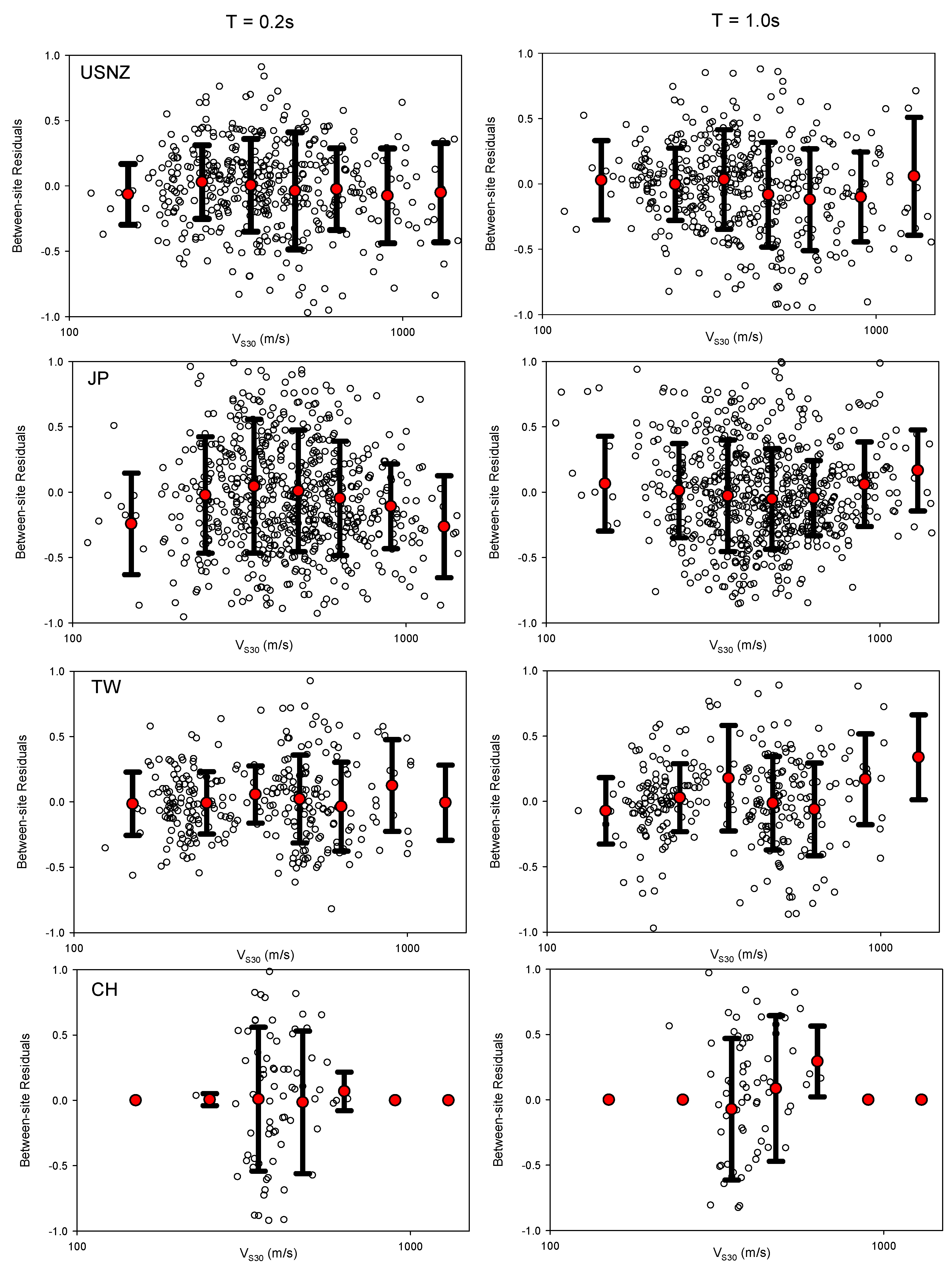
Figure 9.
Between-site residuals at T = 0.2 s and 1 s for each region.


Figure 10.
Variability of site amplification for VS30 and PSArock at T = 0.2 s and 1.0 s. The site bins are: very soft sites (VS30 ≤ 200 m/s), soft sites (200 < VS30 ≤ 300 m/s), stiff sites (300 < VS30 ≤ 400 m/s), moderate stiff sites (400 < VS30 ≤ 550 m/s), very stiff sites (550 < VS30 ≤ 800 m/s), and rock sites (VS30 > 800 m/s). The input rock motion bins for T = 0.2 s are: very weak motion (PSArock < 0.05 g), weak motion (0.05 ≤ PSArock < 0.15 g), moderate motion (0.15 ≤ PSArock < 0.45 g), strong motion (0.45 ≤ PSArock < 0.75 g), and very strong motion (PSArock ≥ 0.75 g). For T = 1.0 s they are: very weak motion (PSArock < 0.01 g), weak motion (0.01 < PSArock < 0.05 g), moderate motion (0.05 < PSArock < 0.10 g), strong motion (0.10 < PSArock < 0.20 g), and very strong motion (PSArock > 0.20 g).


Table 1.
Standard deviation model of the site model.
| Larger Flinn-Engdahl Seismic Regions | Acronym |
|---|---|
| Oregon, California and Nevada * | USNZ |
| New Zealand Region | USNZ |
| Guam to Japan | JP |
| Japan-Kuril Islands-Kamchatka Peninsula | JP |
| Southwestern Japan and Ryukyu Islands | JP |
| Eastern Asia | JP |
| Taiwan | TW |
| Indıa-Xizang-Sichuan-Yunnan | CH |
| Western Asia ** | WA |
| Middle East-Crimea-Eastern Balkans | TRGR |
| Western Mediterranean area *** | WMT |
| Northwestern Europe | NWE |
* Including Alaska, ** Including western Caucasus and Armenia, *** Including northern Italy.
Table 2.
Site model coefficients. The period independent b4 and b5 are 2 and 11, respectively.
| T (s) | b1 | b2 | b3 | σs | c0 | c1 | c2 |
|---|---|---|---|---|---|---|---|
| 0.01 | −0.53307 | −0.46412 | 0.02105 | 0.47096 | 1.24013 | 0.09542 | −0.05865 |
| 0.025 | −0.50842 | −0.3904 | 0.02023 | 0.47508 | 1.24682 | 0.09906 | −0.05951 |
| 0.04 | −0.45025 | −0.31255 | 0.01858 | 0.48906 | 1.33552 | 0.12324 | −0.06481 |
| 0.05 | −0.38023 | −0.23187 | 0.02029 | 0.50412 | 1.6779 | 0.18762 | −0.08741 |
| 0.07 | −0.3505 | −0.18413 | 0.02376 | 0.50892 | 1.57403 | 0.12994 | −0.0791 |
| 0.1 | −0.42752 | −0.37652 | 0.03221 | 0.49777 | 1.52282 | 0.12604 | −0.07408 |
| 0.15 | −0.55919 | −0.53679 | 0.03248 | 0.47977 | 1.31863 | 0.11085 | −0.05612 |
| 0.2 | −0.6673 | −0.6571 | 0.02956 | 0.46896 | 1.21025 | 0.10065 | −0.04777 |
| 0.25 | −0.73135 | −0.69189 | 0.02516 | 0.45698 | 1.13978 | 0.07837 | −0.03958 |
| 0.3 | −0.7884 | −0.68208 | 0.03152 | 0.45065 | 1.05645 | 0.04621 | −0.03245 |
| 0.35 | −0.8332 | −0.69252 | 0.03233 | 0.44141 | 1.01481 | 0.05533 | −0.02765 |
| 0.4 | −0.8681 | −0.74537 | 0.03521 | 0.43589 | 1.00182 | 0.05914 | −0.02363 |
| 0.45 | −0.88575 | −0.73547 | 0.03923 | 0.42954 | 0.94803 | 0.06557 | −0.0179 |
| 0.5 | −0.89944 | −0.69269 | 0.04159 | 0.42699 | 0.94724 | 0.06067 | −0.0171 |
| 0.6 | −0.91493 | −0.6348 | 0.0458 | 0.41593 | 0.95504 | 0.07576 | −0.01606 |
| 0.7 | −0.93236 | −0.63204 | 0.04993 | 0.40303 | 1.01362 | 0.08323 | −0.01527 |
| 0.75 | −0.93217 | −0.6378 | 0.04989 | 0.40219 | 1.03634 | 0.08203 | −0.01622 |
| 0.8 | −0.92975 | −0.65092 | 0.05114 | 0.39766 | 1.05807 | 0.08385 | −0.01434 |
| 0.9 | −0.92777 | −0.57775 | 0.05266 | 0.38861 | 1.11036 | 0.09388 | −0.01658 |
| 1 | −0.93815 | −0.60041 | 0.05421 | 0.3815 | 1.16634 | 0.09095 | −0.01502 |
| 1.2 | −0.93377 | −0.56801 | 0.05576 | 0.36982 | 1.29484 | 0.08078 | −0.01434 |
| 1.4 | −0.93847 | −0.48684 | 0.05782 | 0.35868 | 1.32222 | 0.08353 | −0.00681 |
| 1.6 | −0.92242 | −0.40484 | 0.05645 | 0.35713 | 1.30431 | 0.07158 | −0.00268 |
| 1.8 | −0.91608 | −0.29053 | 0.05615 | 0.34643 | 1.35426 | 0.07341 | 0 |
| 2 | −0.90369 | −0.18149 | 0.05307 | 0.34133 | 1.38763 | 0.0679 | 0 |
| 2.5 | −0.89442 | −0.04175 | 0.05954 | 0.3396 | 1.41986 | 0.08582 | 0 |
| 3 | −0.87386 | 0 | 0.05596 | 0.35349 | 1.37795 | 0.10208 | 0 |
| 3.5 | −0.8551 | 0 | 0.05469 | 0.35286 | 1.34678 | 0.07501 | 0 |
| 4 | −0.8468 | 0 | 0.05469 | 0.36845 | 1.2583 | 0.05876 | 0 |
Table 3.
Site model coefficients for regional effects.
| T (s) | ck,USNZ | ck,JP | ck,TW | ck,CH | ck,WA | ck,GRTR | ck,WMT | ck,NWE |
|---|---|---|---|---|---|---|---|---|
| 0.01 | −0.0302 | 0.0117 | −0.0233 | 0.0158 | 0.1001 | −0.0118 | 0.0172 | 0.0314 |
| 0.025 | −0.0303 | 0.0135 | −0.0272 | 0.015 | 0.1013 | −0.01 | 0.0174 | 0.0264 |
| 0.04 | −0.0336 | 0.0298 | −0.0394 | 0.0111 | 0.1059 | −0.0148 | 0.0101 | 0.0178 |
| 0.05 | −0.04 | 0.0575 | −0.0541 | 0.0099 | 0.1071 | −0.024 | −0.0093 | 0.0038 |
| 0.07 | −0.0346 | 0.0508 | −0.056 | −0.0012 | 0.1119 | −0.019 | −0.0114 | −0.0206 |
| 0.1 | −0.0287 | 0.0199 | −0.045 | 0.022 | 0.1251 | −0.0095 | 0.0084 | −0.0222 |
| 0.15 | −0.0187 | −0.0228 | −0.0114 | 0.0143 | 0.1105 | 0.0044 | 0.0258 | −0.0307 |
| 0.2 | −0.0196 | −0.0439 | 0.0089 | 0.0056 | 0.1134 | 0.0133 | 0.035 | −0.0254 |
| 0.25 | −0.0227 | −0.0543 | 0.0222 | 0.0059 | 0.1016 | 0.0162 | 0.048 | 0.0274 |
| 0.3 | −0.0216 | −0.0583 | 0.03 | −0.00003 | 0.086 | 0.0153 | 0.058 | 0.0407 |
| 0.35 | −0.0187 | −0.0583 | 0.0301 | 0.0025 | 0.089 | 0.0135 | 0.0534 | 0.065 |
| 0.4 | −0.0239 | −0.0544 | 0.0313 | 0.008 | 0.09462 | 0.007 | 0.05177 | 0.0728 |
| 0.45 | −0.0254 | −0.0502 | 0.0327 | 0.0142 | 0.0999 | 0.0041 | 0.0519 | 0.0798 |
| 0.5 | −0.0322 | −0.0461 | 0.036 | 0.0156 | 0.1073 | −0.0022 | 0.0553 | 0.0879 |
| 0.6 | −0.0388 | −0.0389 | 0.0356 | 0.0163 | 0.1209 | −0.0125 | 0.0565 | 0.0978 |
| 0.7 | −0.0411 | −0.0333 | 0.0336 | 0.022 | 0.1246 | −0.0197 | 0.0483 | 0.1104 |
| 0.75 | −0.0416 | −0.0305 | 0.0339 | 0.0252 | 0.1224 | −0.0269 | 0.0485 | 0.1166 |
| 0.8 | −0.0436 | −0.0289 | 0.0346 | 0.0297 | 0.1244 | −0.0321 | 0.0512 | 0.1193 |
| 0.9 | −0.0412 | −0.0262 | 0.0289 | 0.0325 | 0.1239 | −0.0408 | 0.0574 | 0.1303 |
| 1 | −0.0397 | −0.0195 | 0.0146 | 0.0375 | 0.1273 | −0.0434 | 0.0673 | 0.1369 |
| 1.2 | −0.0395 | −0.0071 | −0.0025 | 0.0463 | 0.1376 | −0.0467 | 0.0668 | 0.0914 |
| 1.4 | −0.0365 | −0.0036 | −0.0115 | 0.0574 | 0.1397 | −0.0446 | 0.064 | 0.0893 |
| 1.6 | −0.0361 | 0.0073 | −0.0188 | 0.062 | 0.1319 | −0.0473 | 0.06 | 0.0914 |
| 1.8 | −0.0307 | 0.0108 | −0.0252 | 0.0609 | 0.1332 | −0.0452 | 0.0523 | 0.1062 |
| 2 | −0.028 | 0.0129 | −0.0328 | 0.0591 | 0.1408 | −0.0445 | 0.041 | 0.1092 |
| 2.5 | −0.0336 | 0.0277 | −0.0413 | 0.0588 | 0.1471 | −0.0316 | 0.0197 | 0.0509 |
| 3 | −0.0325 | 0.0369 | −0.0579 | 0.0566 | 0.1679 | −0.0268 | 0.0138 | 0.105 |
| 3.5 | −0.0272 | 0.0461 | −0.063 | 0.0525 | 0.1422 | −0.0294 | 0.0216 | 0.156 |
| 4 | −0.0203 | 0.0503 | −0.0641 | 0.0572 | 0.1945 | −0.0242 | 0.0138 | 0.2198 |
© 2018 by the authors. Licensee MDPI, Basel, Switzerland. This article is an open access article distributed under the terms and conditions of the Creative Commons Attribution (CC BY) license (http://creativecommons.org/licenses/by/4.0/).
Share and Cite
MDPI and ACS Style
Sandıkkaya, M.A.; Dinsever, L.D. A Site Amplification Model for Crustal Earthquakes. Geosciences 2018, 8, 264. https://doi.org/10.3390/geosciences8070264
AMA Style
Sandıkkaya MA, Dinsever LD. A Site Amplification Model for Crustal Earthquakes. Geosciences. 2018; 8(7):264. https://doi.org/10.3390/geosciences8070264
Chicago/Turabian StyleSandıkkaya, M. Abdullah, and L. Doğan Dinsever. 2018. "A Site Amplification Model for Crustal Earthquakes" Geosciences 8, no. 7: 264. https://doi.org/10.3390/geosciences8070264
Note that from the first issue of 2016, this journal uses article numbers instead of page numbers. See further details here.