Street Choice Logit Model for Visitors in Shopping Districts

Abstract
:1. Introduction
2. Method
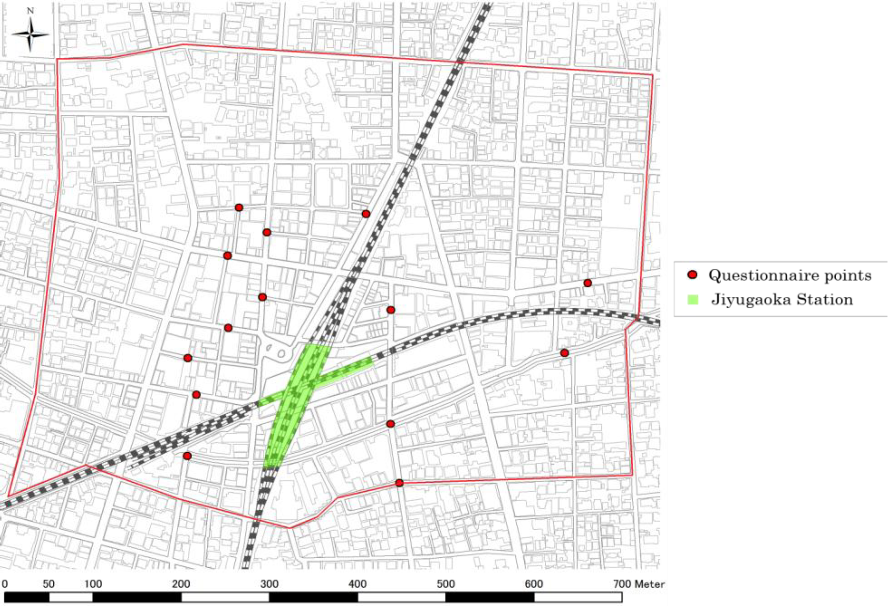
2.1. Study Area

2.2. Variables of Two Models

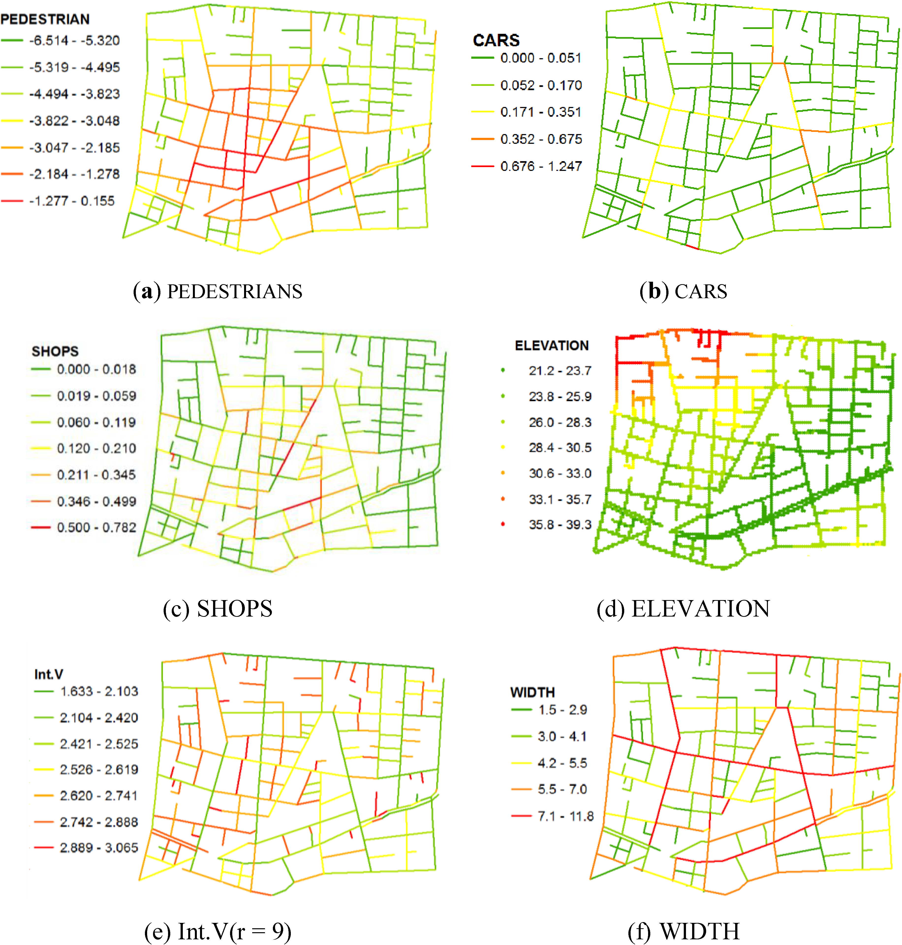
| Variables | Method of data collection |
|---|---|
| PEDESTRIANS | Field survey |
| CARS | |
| SHOPS | Town Pages (NTT yellow pages) |
| ELEVATION | Digital map 5m mesh (elevation) |
| DISTANCE | A program using Dijkstra’s algorithm |
| Int.V | Space Syntax |
| WIDTH | Measuring result (field survey) |
| DIRECTION | questionnaire survey (0 or 1) |
| Retail shops | Service shops | Total | |||||||
|---|---|---|---|---|---|---|---|---|---|
| Commodity | Fashion | General goods | Food | Restaurant | Café | Beauty salon | Beauty parlor | School | |
| 44 | 244 | 131 | 77 | 268 | 35 | 92 | 123 | 107 | 1121 |

3. Pedestrian Distribution Model
| SHOPS | CARS | ELEVATION | DISTANCE | |
|---|---|---|---|---|
| SHOPS | 0.287 ** | −0.060 | −0.281 ** | |
| CARS | −0.035 | 0.770 | ||
| ELEVATION | 0.151 ** |
| Int.V | R-value | R2-value | Adjusted R2-value | Standard error (SE) |
|---|---|---|---|---|
| Axial R3 | 0.719 | 0.518 | 0.504 | 0.403 |
| Axial R5 | 0.722 | 0.521 | 0.508 | 0.402 |
| Axial R7 | 0.725 | 0.525 | 0.512 | 0.400 |
| Axial R9 | 0.728 | 0.530 | 0.517 | 0.398 |
| Axial Rn | 0.727 | 0.529 | 0.515 | 0.399 |
| Angular_R1 | 0.707 | 0.500 | 0.487 | 0.410 |
| Angular_R2 | 0.709 | 0.503 | 0.489 | 0.409 |
| Angular_R3 | 0.710 | 0.505 | 0.491 | 0.409 |
| Angular_R4 | 0.710 | 0.504 | 0.490 | 0.409 |
| Angular_R5 | 0.710 | 0.504 | 0.490 | 0.409 |
| Angular_Rn | 0.709 | 0.503 | 0.490 | 0.409 |
| Metric_150m | 0.716 | 0.513 | 0.500 | 0.405 |
| Metric_300m | 0.722 | 0.521 | 0.508 | 0.402 |
| Metric_450m | 0.724 | 0.524 | 0.510 | 0.401 |
| Metric_600m | 0.717 | 0.514 | 0.501 | 0.404 |
| Metric_750m | 0.716 | 0.513 | 0.499 | 0.405 |
| Metric_900m | 0.712 | 0.508 | 0.494 | 0.407 |
| Metric_1050m | 0.707 | 0.500 | 0.486 | 0.411 |
| Explanatory variable | Non-Standardizing Coefficient | Standardizing Coefficient | p-value | Collinearity | |||
|---|---|---|---|---|---|---|---|
| Partial regression coefficient | Standard Error | Standardised partial regression coeficient | t-value | Tolerance | Variance Inflation Factor | ||
| Constant | −1.799 | 0.433 | −4.158 | 0.000 | |||
| Int.V | 0.923 | 0.269 | 0.192 | 3.426 | 0.001 | 0.829 | 1.206 |
| SHOPS | 0.707 | 0.128 | 0.311 | 5.538 | 0.000 | 0.825 | 1.212 |
| CARS | 1.375 | 0.853 | 0.089 | 1.612 | 0.109 | 0.854 | 1.171 |
| ELEVATION | −0.046 | 0.010 | −0.265 | −4.835 | 0.000 | 0.862 | 1.160 |
| DISTANCE | −0.002 | 0.000 | −0.417 | −7.476 | 0.000 | 0.832 | 1.201 |
4. Street Choice Model
4.1. Questionnaire Survey on the Visitors’ Strolling Route
| Items | Choices |
|---|---|
| Gender | Male, Female |
| Age | Teens, Twenties, Thirties, Forties, Fifties, Sixties, Other |
| Purpose | Shopping, Lunch, Rambling, Business, Get home, Other |
| Transportation mode | On foot, Bicycle, Bus, Train, Car |
| Travel time | < 30 min, 30 min, 1 h, 1.5 h, 2 h |
| Frequency | Once, Twice, Third times, Other, |
| Relationships | Friend, Parent, Couple, Other |
| Stationary time | Free answer |
| Route | Free answer |
| Attribution | Definition | Number of choices | Rambling ratio |
|---|---|---|---|
| All | All street choices | 1211 | 34% |
| Toward destination (TD) | Heading for destination | 799 | 0% |
| Non-destination (ND) | Undefined destinations | 412 | 100% |
| Male | Only male (alone, group) | 230 | 40% |
| Female | Only female (alone, group) | 825 | 30% |
| Couple | Male and female group | 156 | 46% |
| Alone | Street choices for alone person | 129 | 30% |
| Group | Street choices for a group | 780 | 36% |
4.2. Logit Model


4.3. Estimated Parameters for Each Attribute
| Attribution | Int.V | SHOPS | CARS | ELEVATION | WIDTH | DISTANCE | DIRECTION | HR (%) |
|---|---|---|---|---|---|---|---|---|
| All | 0.725 | 1.235 *** | −3.695 | −0.160 ** | 0.104 *** | −0.052 *** | −1.354 *** | 80 |
| TD | −0.939 | 1.952 *** | −7.181 | −0.262 ** | 0.132 *** | −0.534 *** | −1.238 *** | 87 |
| ND | 2.010 ** | 0.582 | −2.822 | −0.122 | 0.071 | −1.485 *** | 67 | |
| Male | 2.771 * | 2.558 ** | −12.929* | −0.148 | 0.265 *** | −0.067 *** | −1.635 *** | 85 |
| Female | 0.565 | 1.155 ** | −3.175 | −0.060 | 0.095 ** | −0.055 *** | −1.282 *** | 80 |
| Couple | 0.283 | 0.957 | 3.363 | −0.506 *** | 0.038 | −0.042 *** | −1.484 *** | 77 |
| Alone | 1.881 * | 2.411 *** | −15.222 ** | −0.222 * | 0.188 *** | −0.068 *** | −1.469 *** | 84 |
| Group | 0.068 | 0.867 ** | 0.636 | −0.128 | 0.074 * | −0.048 *** | −1.334 *** | 78 |
5. Conclusions
Acknowledgments
Author Contributions
Conflicts of Interest
References
- Gil, J.; Tobari, E.; Lemlij, M.; Rose, A.; Penn, A. The Differentiating Behaviour of Shoppers Clustering of Individual Movement Traces in a Supermarket. In Proceedings of the 7th International Space Syntax Symposium, Stockholm, Sweden, 8–11 June 2009.
- Millonig, A.; Schechtner, K. Understanding Walking Behaviour—Pedestrian Motion Patterns and Preferences in Shopping Environments. Available online: http://www.walk21.com/papers/Alexandra%20Millonig%20and%20Katja%20Schechtnerb_Understanding%20Walking%20Behaviour.Pedestrian%20Motion%20Patterns%20and%20Preferences%20in%20Shopping%20Environments.pdf (accessed on 2 June 2014).
- Tsukaguchi, H.; Matsuda, K. Analysis on Pedestrian Route Choice Behavior. J. Infrastruct. Plan. Manag. 2002, 56, 117–126. [Google Scholar]
- Golledge, R.G. Defining the Criteria Used in Path Selection. Working Paper No. 278. Transportation Center, The University of California: Berkeley, CA, USA, 1995; pp. 1–37. Available online: http://www.uctc.net/papers/278.pdf (accessed on 2 June 2014).
- Golledge, R.G. “Path Selection and Route Preference in Human Navigation—A Progress Report.”. Working Paper No. 277. Transportation Center, University of California: Berkeley, CA, 1995; pp. 207–222. Available online: http://www.uctc.net/papers/277.pdf (accessed on 2 June 2014).
- Takegami, N.; Tsugaguchi, H. Modeling of Pedestrian Route Choice Behavior Based on The Spatial Relationship Between The Pedestrian’s Current Location and The Destination. J. Infrastruct. Plan. Manag. 2006, 62, 64–73. [Google Scholar] [CrossRef]
- Kneidl, A.; Borrmann, A. How Do Pedestrians Find their Way? Results of an Experimental Study with Students Compared to Simulation Results. In Proceedings of Emergency Evacuation of People from Buildings, Warsaw, Poland, 31 March 2010.
- Sakurai, Y.; Koshizuka, T. Estimation of Pedestrian Flow in Toyohashi City. J. Plan. Inst. Jpn. 2012, 47, 817–822. [Google Scholar]
- Zhu, W.; Timmermans, H. Modeling Pedestrian Shopping Behavior Using Principles of Bounded Rationality: Model Comparison and Validation. J. Geogr. Sci. 2011, 13, 101–126. [Google Scholar]
- Sueshige, Y.; Morozumi, M. The Visual Information Which Encourage or Restrain Citizens’ Strolling Activities in Urban Space: On the relationship of strolling activities and visual information given by the environment in downtown Kumamoto Part 2. J. Archit. Plan. 2007, 614, 191–197. [Google Scholar]
- Oiwa, Y.; Yamada, T.; Misaka, T.; Kaneda, T. A Transition Analysis of Shopping District from the View Point of Visitors’ Shop around Behaviors: A Case Study of Ohsu Distinct, Nagoya (Urban Planning). J. Archit. Build. Sci. 2005, 22, 469–474. [Google Scholar]
- Kawanabe, M.; Kawashima, K. A Study on Rambling Activities of Visitor by Tram in Central Commercial District: Focusing on Behavioral Characteristics of Visitor and Spatial Composition in Hiroshima City. J. Plan. Inst. Jpn. 2012, 47, 168–174. [Google Scholar]
- Matsumoto, N.; Funabiki, E. Relationship between Foot Passengers’ Actions of Stop without Purpose and Stop with Purpose in an Underground Shopping Arcade. J. Archit. Plan. 2011, 76, 321–326. [Google Scholar] [CrossRef]
- Hensher, D.A.; Rose, J.M.; Greene, W.H. Applied Choice Analysis; Cambridge University Press: Tokyo, Japan, 2005. [Google Scholar]
- Japan Society of Civil Engineers. Hishuukei Koudou Logit-model No Riron to Jissai; Japan Society of Civil Engineers: Tokyo, Japan, 1995. (In Japanese) [Google Scholar]
© 2014 by the authors; licensee MDPI, Basel, Switzerland. This article is an open access article distributed under the terms and conditions of the Creative Commons Attribution license (http://creativecommons.org/licenses/by/3.0/).
Share and Cite
Kawada, K.; Yamada, T.; Kishimoto, T. Street Choice Logit Model for Visitors in Shopping Districts. Behav. Sci. 2014, 4, 154-166. https://doi.org/10.3390/bs4030154
Kawada K, Yamada T, Kishimoto T. Street Choice Logit Model for Visitors in Shopping Districts. Behavioral Sciences. 2014; 4(3):154-166. https://doi.org/10.3390/bs4030154
Chicago/Turabian StyleKawada, Ko, Takashi Yamada, and Tatsuya Kishimoto. 2014. "Street Choice Logit Model for Visitors in Shopping Districts" Behavioral Sciences 4, no. 3: 154-166. https://doi.org/10.3390/bs4030154