
Seasonal Variations in the Use of Profundal Habitat among Freshwater Fishes in Lake Norsjø, Southern Norway, and Subsequent Effects on Fish Mercury Concentrations

Abstract
:1. Introduction
2. Materials and Methods
2.1. Sampled Fish
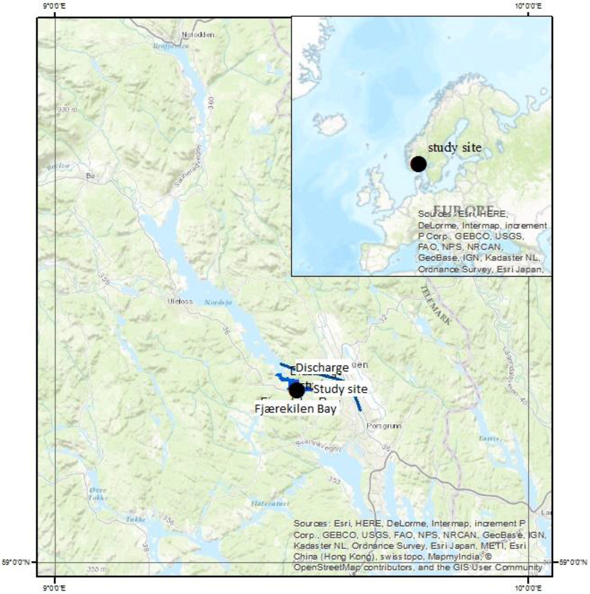
2.2. Site Description
2.3. Sampling
2.4. General Analysis
2.5. Benthic Invertebrates and Stomach Content Analysis
2.6. Preparation of Muscle Fillet Samples for SI and Hg Analysis
2.7. Stable Isotope Analysis
2.8. Hg Analysis
2.9. Data Analysis
3. Results
3.1. Descriptive Statistics
3.2. Use of the Profundal Habitat
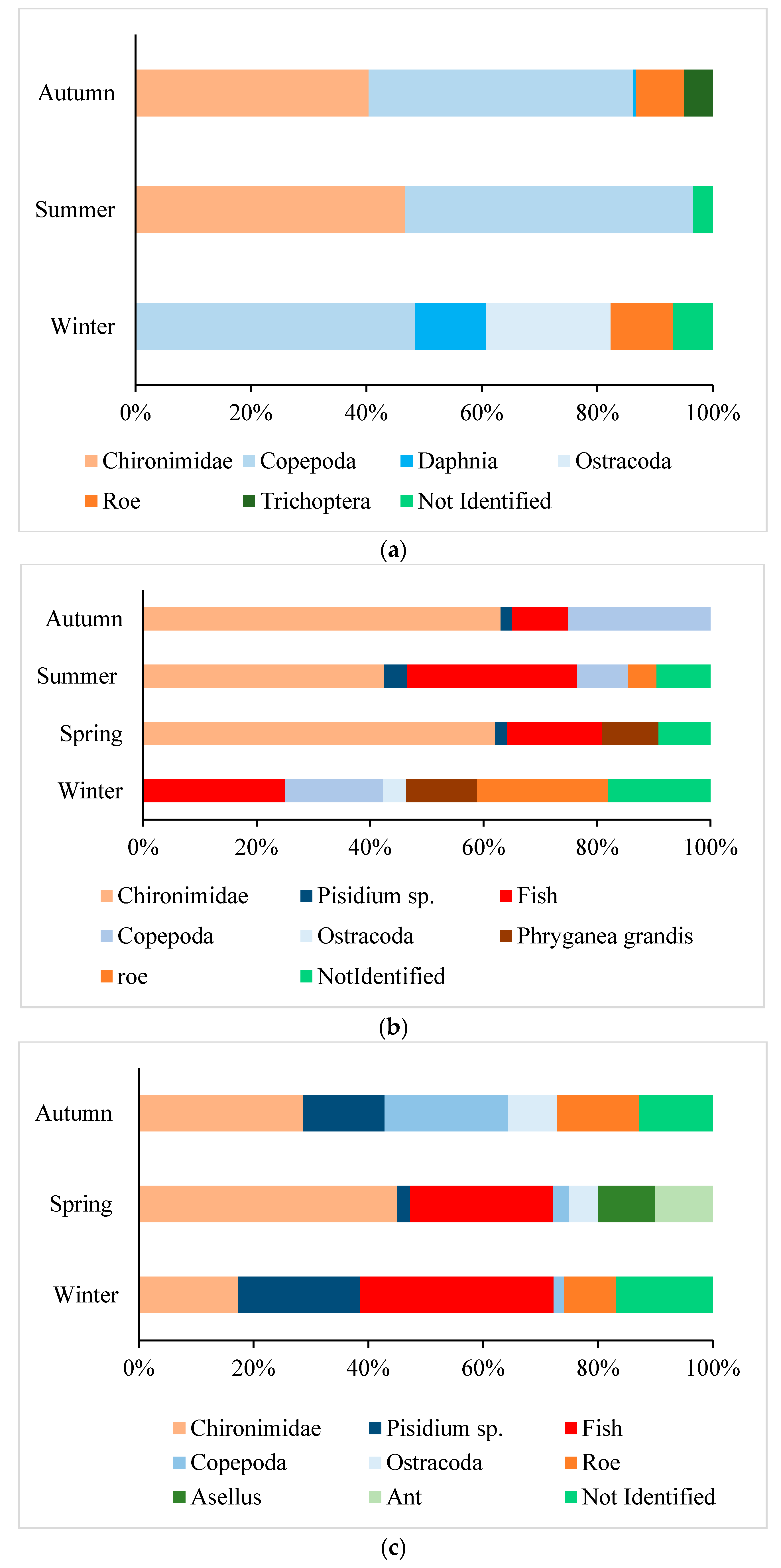
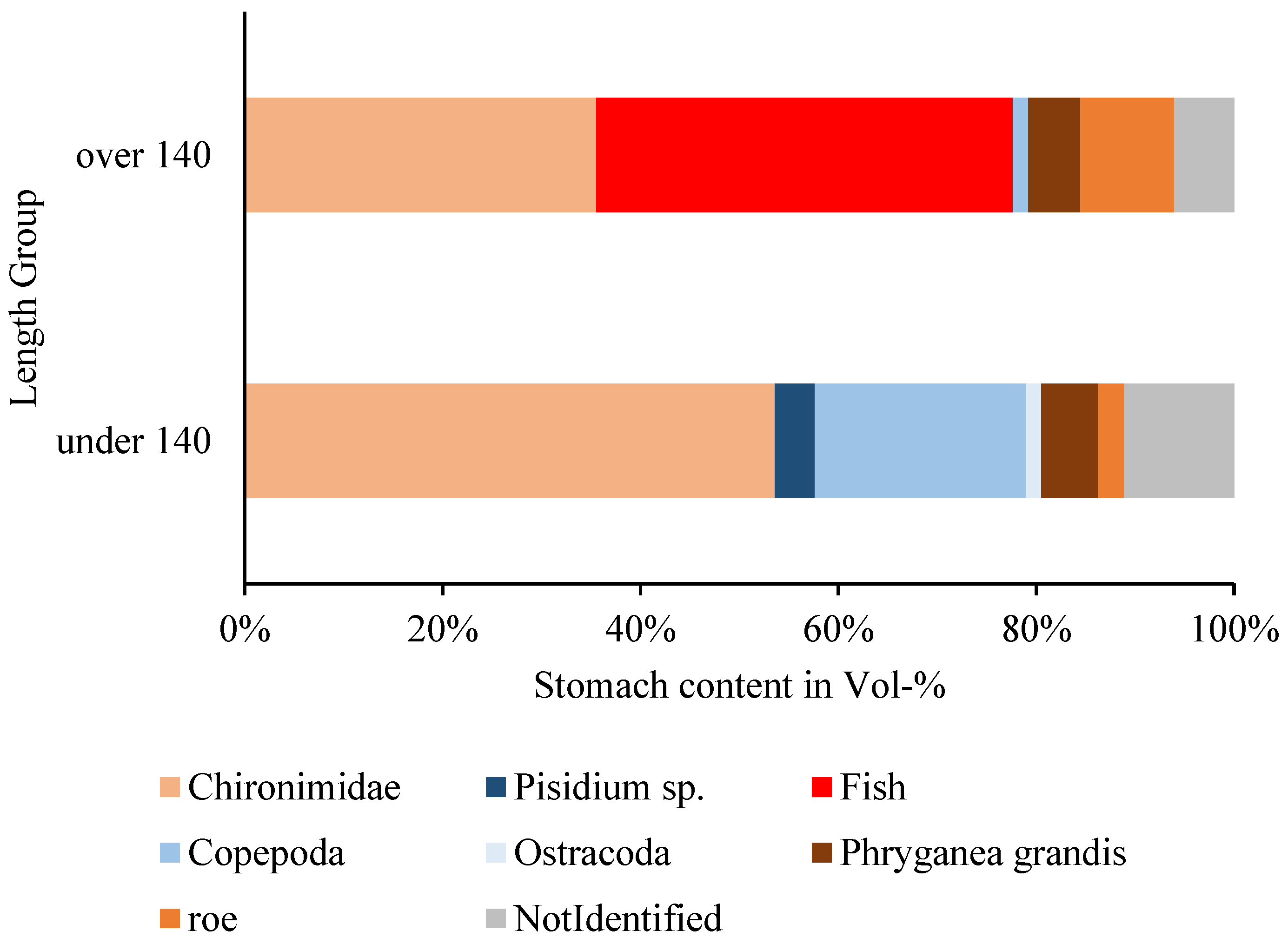
3.3. Stomach Content and Diet
3.3.1. Benthic Invertebrates
3.3.2. Pelagic Invertebrates
3.3.3. Fish and Other Items
3.4. Hg-Models
3.4.1. Model Intercepts and Residual Standard Error
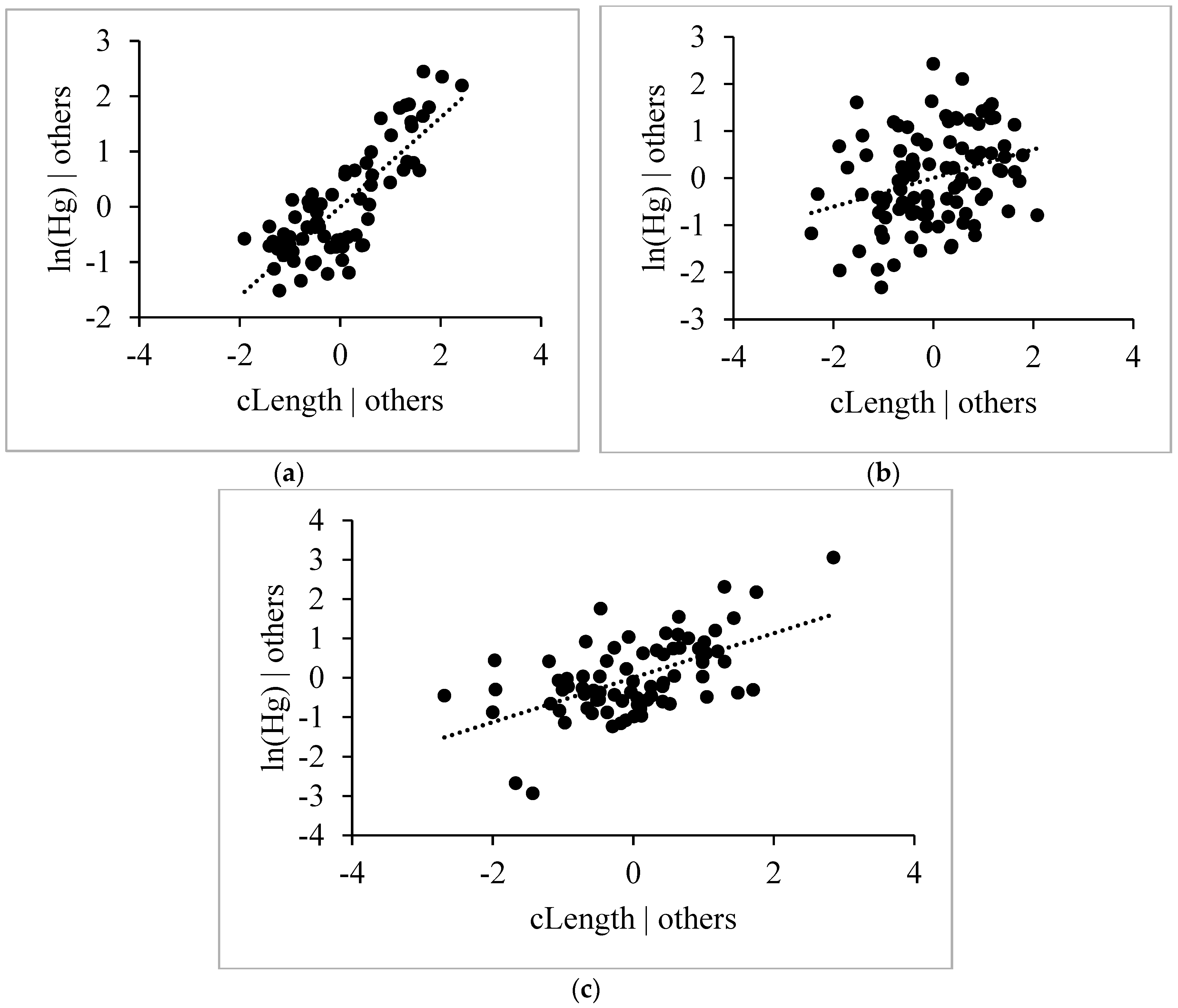
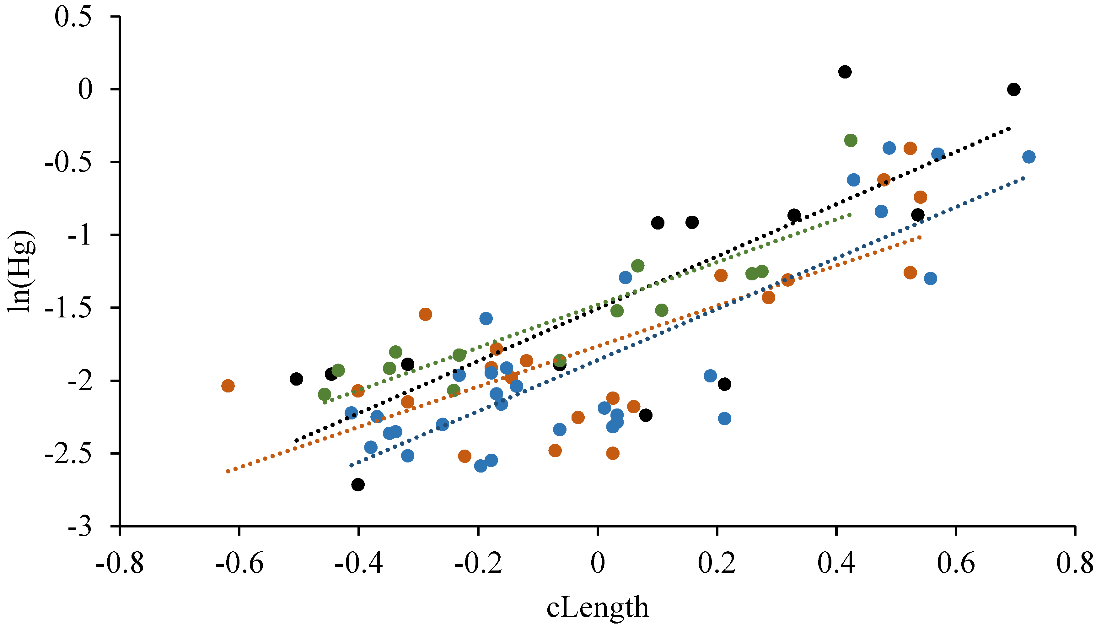
3.4.2. Length
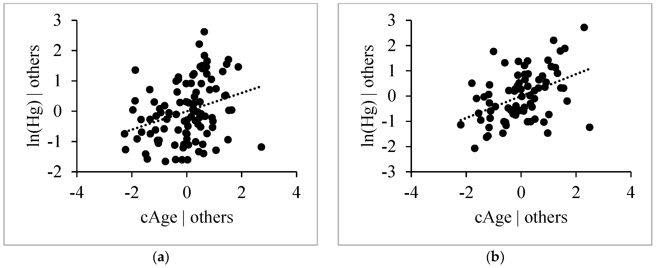
3.4.3. Age
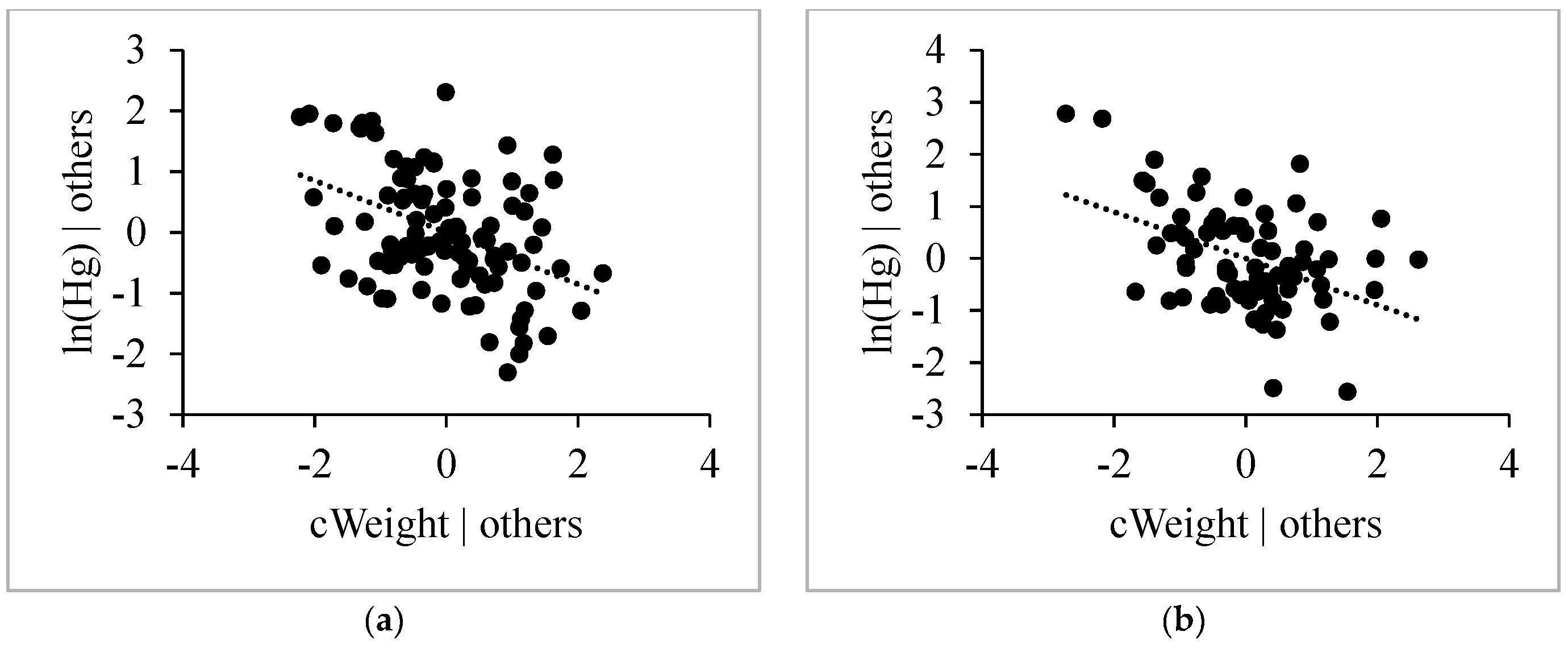
3.4.4. Weight
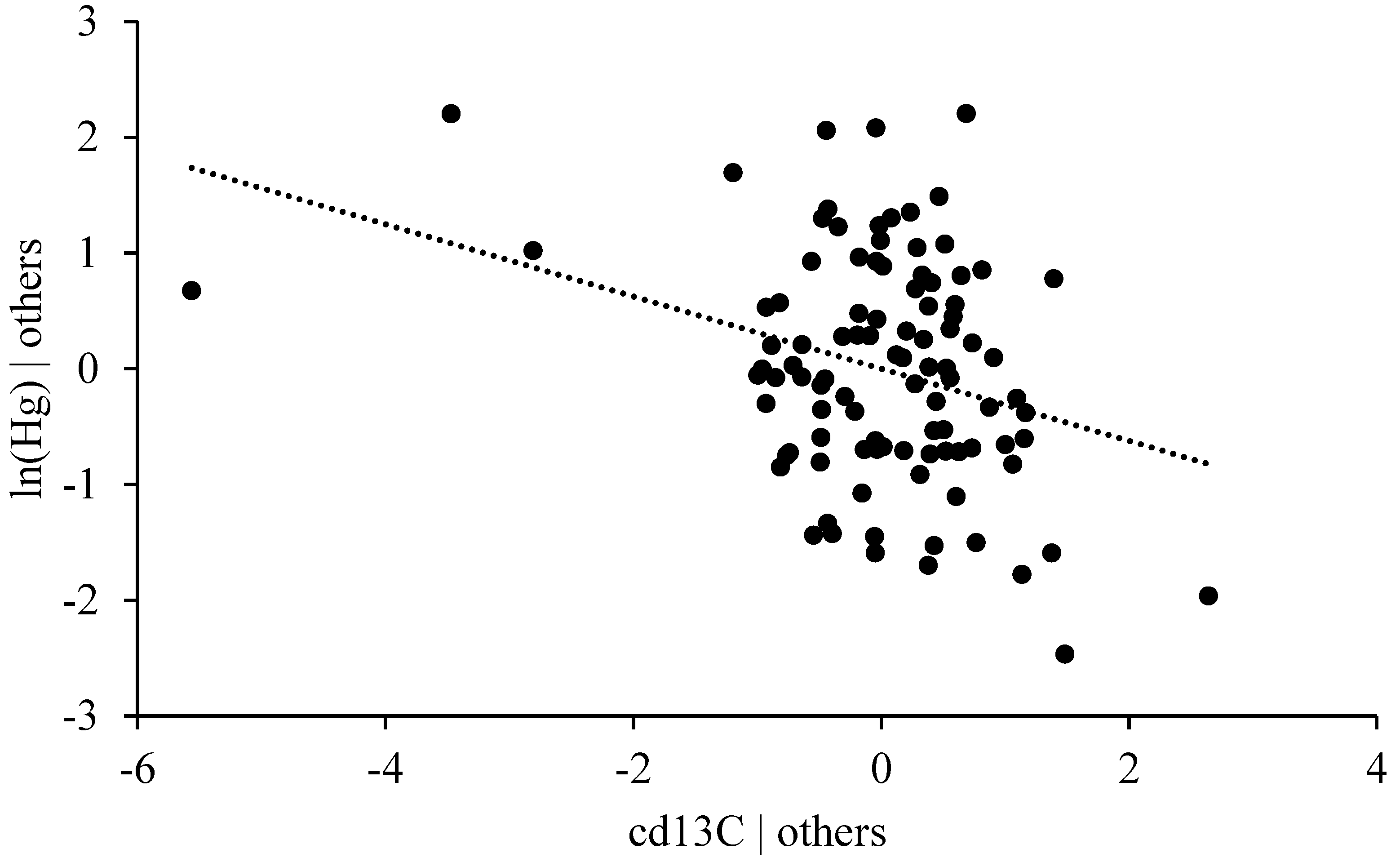
3.4.5. Stable Isotope Ratio δ13C
3.4.6. Stable Isotope Ratio δ15N
3.4.7. Season
4. Discussion
4.1. Age, Size and Weight Distributions, Stable Isotope Ratios and Tot-Hg
4.2. Use of the Profundal Habitat
4.3. Ontogenetic Diet Shift in A. Charr
4.4. Factors Determining Tot-Hg-Concentrations (Model Results)
4.4.1. Length, Age and Weight
4.4.2. Habitat Effect and δ13C
4.4.3. Biomagnification and δ15N
4.4.4. Seasonal Variation
5. Conclusions
Supplementary Materials
Acknowledgments
Author Contributions
Conflicts of Interest
Abbreviations
| ABD | Algal bloom dilution |
| AIC | Akaike information criterion |
| Df | Degrees of freedom |
| Gls | Generalised least squares |
| Hg | Mercury |
| ML | Maximum likelihood |
| ppm | Parts per million |
| REML | Restricted maximum likelihood |
| SD | Standard deviation |
| SE | Standard error |
| SGD | Somatic growth dilution |
| Tot-Hg | Total Mercury |
| ww. | Wet weight |
References
- Gilmour, C.C.; Riedel, C.S. Measurement of Hg methylation in sediments using high specific-activity Hg-203 and ambient incubator. Water Air Soil Pollut. 1995, 80, 747–756. [Google Scholar] [CrossRef]
- Macalady, J.L.; Mack, E.E.; Nelson, D.C.; Scow, K.M. Sediment microbial community structure and mercury methylation in mercury-polluted clear lake, California. Appl. Environ. Microbiol. 2000, 66, 1479–1488. [Google Scholar] [CrossRef] [PubMed]
- Hollweg, T.A.; Gilmour, C.C.; Mason, R.P. Mercury and methylmercury cycling in sediments of the mid-Atlantic continental shelf and slope. Limnol. Oceanogr. 2010, 55, 2703–2722. [Google Scholar] [CrossRef]
- Lehnherr, I.; St. Louis, V.L.; Kirk, J.L. Methylmercury cycling in high arctic wetland ponds: Controls on sedimentary production. Environ. Sci. Technol. 2012, 46, 10523–10531. [Google Scholar] [CrossRef] [PubMed]
- Cabana, G.; Rasmussen, J.B. Modeling food-chain structure and contaminant bioaccumulation using stable nitrogen isotopes. Nature 1994, 372, 255–257. [Google Scholar] [CrossRef]
- Atwell, L.; Hobson, K.A.; Welch, H.E. Biomagnification and bioaccumulation of mercury in an arctic marine food web: Insights from stable nitrogen isotope analysis. Can. J. Fish. Aquat. Sci. 1998, 55, 1114–1121. [Google Scholar] [CrossRef]
- Watras, C.J.; Back, R.C.; Halvorsen, S.; Hudson, R.J.M.; Morrison, K.A.; Wente, S.P. Bioaccumulation of mercury in pelagic freshwater food webs. Sci. Total Environ. 1998, 219, 183–208. [Google Scholar] [CrossRef]
- Eagles-Smith, C.A.; Suchanek, T.H.; Colwell, A.E.; Anderson, N.L. Mercury trophic transfer in a eutrophic lake: The importance of habitat-specific foraging. Ecol. Appl. 2008, 18, A196–A212. [Google Scholar] [CrossRef] [PubMed]
- Kidd, K.; Clayden, M.; Jardine, T. Bioaccumulation and biomagnification of mercury through food webs. In Environmental Chemistry and Toxicology of Mercury; Liu, G., Cai, Y., O’Driscoll, N., Eds.; Wiley: Hoboken, NJ, USA, 2012; pp. 455–499. [Google Scholar]
- Lavoie, R.A.; Jardine, T.D.; Chumchal, M.M.; Kidd, K.A.; Campbell, L.M. Biomagnification of mercury in aquatic food webs: A worldwide meta-analysis. Environ. Sci. Technol. 2013, 47, 13385–13394. [Google Scholar] [CrossRef] [PubMed]
- Stafford, C.P.; Hansen, B.; Stanford, J.A. Mercury in fishes and their diet items from Flathead Lake, Montana. Trans. Am. Fish. Soc. 2004, 133, 349–357. [Google Scholar] [CrossRef]
- Huckabee, J.W.; Elwood, J.W.; Hildebrand, S.G. Accumulation of mercury in freshwater biota. In Biogeochemistry of Mercury in the Environment; Nriago, J.O., Ed.; Elsevier/North-Holland Biomedical Press: New York, NY, USA, 1979; pp. 277–302. [Google Scholar]
- Driscoll, C.T.; Yan, C.; Schofield, C.L.; Munson, R.; Holsapple, J. The mercury cycle and fish in the Adirondack lakes. Environ. Sci. Technol. 1994, 28, 136–143. [Google Scholar] [CrossRef]
- Cidzdziel, J.V.; Hinners, T.A.; Pollard, J.E.; Heithmar, E.M.; Cross, C.L. Mercury concentrations in fish from Lake Mead, USA, related to fish size, condition, trophic level, location and consumption risk. Arch. Environ. Contam. Toxicol. 2002, 43, 309–317. [Google Scholar] [CrossRef] [PubMed]
- Thomann, R.V. Bioaccumulation model of organic chemical distribution in aquatic food chains. Environ. Sci. Technol. 1989, 23, 699–707. [Google Scholar] [CrossRef]
- Verta, M. Changes in fish mercury concentrations in an intensively fished lake. Can. J. Fish. Aquat. Sci. 1990, 47, 1888–1897. [Google Scholar] [CrossRef]
- Pickhardt, P.C.; Folt, C.L.; Chen, C.Y.; Klaue, B.; Blum, J.D. Algal blooms reduce the uptake of toxic methylmercury in freshwater food webs. Proc. Natl. Acad. Sci. USA 2002, 99, 4419–4423. [Google Scholar] [CrossRef] [PubMed]
- Pickhardt, P.C.; Folt, C.L.; Chen, C.Y.; Klaue, B.; Blum, J.D. Impacts of zooplankton composition and algal enrichment on the accumulation of mercury in an experimental freshwater food web. Sci. Total Environ. 2005, 339, 89–101. [Google Scholar] [CrossRef] [PubMed]
- Karimi, R.; Chen, C.Y.; Pickhardt, P.C.; Fisher, N.S.; Folt, C.L. Stoichiometric controls of mercury dilution by growth. Proc. Natl. Acad. Sci. USA 2007, 104, 7477–7482. [Google Scholar] [CrossRef] [PubMed]
- Ward, D.M.; Nislow, K.H.; Folt, C.L. Bioaccumulation syndrome: Identifying factors that make some stream food webs prone to elevated mercury bioaccumulation. In Year in Ecology and Conservation Biology; Ostfeld, R.S., Schlesinger, W.H., Eds.; The New York Academy of Sciences: New York, NY, USA, 2010; Volume 1195, pp. 62–83. [Google Scholar]
- Lepak, J.M.; Kinzli, K.-D.; Fetherman, E.R.; Pate, W.M.; Hansen, A.G.; Gardunio, E.I.; Cathcart, C.N.; Stacy, W.L.; Underwood, Z.E.; Brandt, M.M.; et al. Manipulation of growth to reduce mercury concentrations in sport fish on a whole-system scale. Can. J. Fish. Aquat. Sci. 2012, 69, 122–135. [Google Scholar] [CrossRef]
- Hobson, K.A.; Alisauskas, R.T.; Clark, R.G. Stable-nitrogen isotope enrichment in avian tissues due to fasting and nutritional stress: Implications for isotopic analysis of diet. Condor 1993, 95, 388–394. [Google Scholar] [CrossRef]
- Meili, M.; Wills, D. Seasonal concentration changes of Hg, Cd, Cu and Al in a population of roach (Rutilus rutilus). In Heavy Metals in the Environment; Lekkas, T.D., Ed.; Commission of the European Communities Consultants: Athens, Greece, 1985; pp. 709–711. [Google Scholar]
- Staveland, G.; Marthinsen, I.; Norheim, G.; Julshamn, K. Levels of environmental pollutants in flounder (Platichthys flesus L.) and cod (Gadus morhua L.) caught in the waterway of Glomma, Norway. II. Mercury and arsenic. Arch. Environ. Contam. Toxicol. 1993, 24, 187–193. [Google Scholar] [CrossRef] [PubMed]
- Park, J.; Curtis, L.R. Mercury distribution in sediments and bioaccumulation by fish in two Oregon reservoirs: Point-source and nonpoint-source impacted systems. Arch. Environ. Contam. Toxicol. 1997, 33, 423–429. [Google Scholar] [CrossRef] [PubMed]
- Gorski, P.R.; Lathrop, R.C.; Hill, S.D.; Herrin, R.T. Temporal mercury dynamics and diet composition in the mimic shiner. Trans. Am. Fish. Soc. 1998, 128, 701–712. [Google Scholar] [CrossRef]
- Farkas, A.; Salánki, J.; Speciár, A. Age- and size-specific patterns on heavy metals in the organs of freshwater fish Abramis brama L., populating a low-contaminated site. Water Res. 2003, 37, 959–964. [Google Scholar] [CrossRef]
- Murphy, G.W.; Newcomb, T.J.; Orth, O.J. Sexual and seasonal variations of mercury in smallmouth bass. J. Freshw. Ecol. 2007, 22, 35–143. [Google Scholar] [CrossRef]
- Zhang, L.; Campbell, L.M.; Johnson, T.B. Seasonal variation in mercury and food web biomagnification in Lake Ontario, Canada. Environ. Pollut. 2012, 161, 178–184. [Google Scholar] [CrossRef] [PubMed]
- Moreno, C.E.; Fjeld, E.; Deshar, M.K.; Lydesen, E. Seasonal variation of mercury and δ15N in fish from Lake Heddalsvatn, southern Norway. J. Limnol. 2015, 74, 21–30. [Google Scholar] [CrossRef]
- Farkas, A.; Saláki, J.; Varanka, I. Heavy metal concentrations in fish of Lake Balaton. Lakes Reserv. 2000, 5, 271–279. [Google Scholar] [CrossRef]
- Foster, E.P.; Drake, D.I.; DiDimenico, G. Seasonal changes and tissue distribution of mercury in largemouth bass (M. ceopterus salmoides) from Dorena Reservoir, Oregon. Arch. Environ. Contam. Toxicol. 2000, 38, 78–82. [Google Scholar] [CrossRef] [PubMed]
- Burger, J.; Jeitner, C.; Donio, M.; Shukla, S.; Gochfeld, M. Factors affecting mercury and selenium levels in New Jersey flatfish: Low risk to human consumers. J. Toxicol. Environ. Health 2009, 72, 853–860. [Google Scholar] [CrossRef] [PubMed]
- Peterson, B.J.; Fry, B. Stable isotopes in ecosystem studies. Ann. Rev. Ecol. Syst. 1987, 18, 293–320. [Google Scholar] [CrossRef]
- Cabana, G.; Rasmussen, J.B. Comparison of aquatic food chains using nitrogen isotopes. Proc. Natl. Acad. Sci. USA 1996, 93, 10844–10847. [Google Scholar] [CrossRef] [PubMed]
- Post, D.M. Using stable isotopes to estimate trophic position: Models, methods, and assumptions. Ecology 2002, 83, 703–718. [Google Scholar] [CrossRef]
- Hoefs, J. Stable Isotope Geochemistry; Springer Science & Business Media: New York, NY, USA, 2013. [Google Scholar]
- Minagawa, M.; Wada, E. Stepwise enrichment of 15N along food chains: Further evidence and the relation between delta15N and animal age. Geochim. Cosmochim. Acta 1984, 48, 1135–1140. [Google Scholar] [CrossRef]
- Vander Zanden, M.J.; Rasmussen, J.B. Primary consumer delta13C and delta15N and the trophic position of aquatic consumers. Ecology 1999, 80, 1395–1404. [Google Scholar] [CrossRef]
- Lavoie, R.A.; Hebert, C.E.; Rail, J.-F.; Braune, B.M.; Yumvihoze, E.; Hill, L.G.; Lean, D.R.S. Trophic structure and mercury distribution in a Gulf of St. Lawrence (Canada) food web using stable isotope analysis. Sci. Total Environ. 2010, 408, 5529–5539. [Google Scholar] [CrossRef] [PubMed]
- Power, M.; Klein, G.M.; Guiguer, K.; Kwan, M.K.H. Mercury accumulation in the fish community of a sub-Arctic lake in relation to trophic position and carbon sources. J. Appl. Ecol. 2002, 39, 819–830. [Google Scholar] [CrossRef]
- Gorski, P.R.; Cleckner, L.B.; Hurley, J.P.; Sierzen, M.E.; Armstrong, D.E. Factors affecting enhanced mercury bioaccumulation in inland lakes of Isle Royale National Park, USA. Sci. Total Environ. 2003, 304, 327–348. [Google Scholar] [CrossRef]
- Stewart, A.R.; Saiki, M.K.; Kuwabara, J.S.; Alpers, C.N.; Marvin-Dipasquale, M.; Krabbenhoft, D.P. Influence of plankton mercury dynamics and trophic pathways on mercury concentrations of top predator fish of a mining-impacted reservoir. Can. J. Fish. Aquat. Sci. 2008, 65, 2351–2366. [Google Scholar] [CrossRef]
- Chumchal, M.M.; Hambright, K.D. Ecological factors regulating mercury contamination of fish from Caddo Lake, Texas, USA. Environ. Toxicol. Chem. 2009, 28, 962–972. [Google Scholar] [CrossRef] [PubMed]
- Holtan, H. Norsjø: En Limnologisk Undersøkelse Utført I 1967; Norwegian Institute for Water Research NIVA: Oslo, Norway, 1968; p. 40. [Google Scholar]
- Vann-Nett. Available online: http://www.vann-nett.no/portal/water?waterbodyID=016-6-L (accessed on 28 July 2016).
- Nordeng, H. On the biology of char (Salmo alpinus L.) in Salangen, North Norway. Age and spawning frequency determined from scales and otoliths. Nytt Mag. Zool. 1961, 10, 67–123. [Google Scholar]
- Shanks, A.L. Surface slicks associated with tidally forced internal waves may transport pelagic larvae of benthic invertebrates and fishes shoreward. Mar. Ecol. Prog. Ser. 1983, 13, 311–315. [Google Scholar] [CrossRef]
- Raastad, J.E.; Olsen, L.-H. Insekter og Småkryp I Vann og Vassdrag; Aschehoughs Naturbøker: Oslo, Norway, 1999. [Google Scholar]
- Craig, H. Isotopic standards for carbon and oxygen and correction factors for mass-spectrometric analysis of carbon dioxide. Geochim. Cosmochim. Acta 1957, 12, 133–149. [Google Scholar] [CrossRef]
- R Core Team. R: A Language and Environment for Statistical Computing; R Foundation for Statistical Computing: Vienna, Austria, 2016. [Google Scholar]
- NLME: Linear and Nonlinear Mixed Effects Models, R-Package Version 3.1-127, 2016. Available online: http://CRAN.R-project.org/package=nlme (accessed on 28 July 2016).
- Zuur, A.F.; Ieno, E.N.; Walker, N.J.; Saveliev, A.A.; Smith, G.M. Mixed Effects Models and Extensions in Ecology with R; Springer Science & Business Media: New York, NY, USA, 2009; p. 574. [Google Scholar]
- RGL: 3D Visualization Using Open GL, R-Package Version 0.95.1441, 2016. Available online: https://CRAN.R-project.org/package=rgl (accessed on 28 July 2016).
- RGLWIDGET: “RGL” in “HTMLWIDGETS” Framework, R-Package Version 0.1.1434, 2015. Available online: https://CRAN.R-project.org/package=rglwidget (accessed on 28 July 2016).
- Schoener, T.W. Nonsynchronous spatial overlap of lizards in patchy habitats. Ecology 1970, 51, 408–418. [Google Scholar] [CrossRef]
- Wallace, R.K. An Assessment of diet overlap indices. Trans. Am. Fish. Soc. 1981, 110, 72–76. [Google Scholar] [CrossRef]
- Nilsson, N.A. Interactive segregation between fish species. In The Biological Basis of Freshwater Fish Production; Gerking, S.D., Ed.; Blackwell Scientific: Oxford, UK, 1967; pp. 295–313. [Google Scholar]
- Amundsen, P.-A.; Knudsen, R.; Bryhni, H.T. Niche use and resource partitioning of Arctic charr, European whitefish and grayling in a subarctic lake. Hydrobiologia 2010, 650, 3–14. [Google Scholar] [CrossRef]
- Borgstrøm, R.; Saltveit, S.J. En Vurdering av Fisketap Gjennom Tappetunnellene fra Nedre Norsjø til Rafnes og Porsgrunn Fabrikker; Institutt for Naturforvaltning NHL: Ås, Norway, 1981; 18p. [Google Scholar]
- Degerman, E.; Hammar, J.; Nyberg, P.; Svardson, G. Human impact on the fish diversity in the four largest lakes of Sweden. Ambio 2001, 30, 522–528. [Google Scholar] [CrossRef] [PubMed]
- Sandlund, O.T.; Haugerud, E.; Rognerud, S.; Borgstrøm, R. Arctic charr (Salvelinus alpinus) squeezed in a complex fish community dominated by Perch (Perca fluviatilis). Fauna Nor. 2013, 33, 1–11. [Google Scholar] [CrossRef]
- Gu, B.; Schell, D.M.; Alexander, V. Stable carbon and nitrogen isotopic analysis of the plankton food web on a subarctic lake. Can. J. Fish. Aquat. Sci. 1994, 51, 1338–1344. [Google Scholar] [CrossRef]
- Yoshioka, T.; Wada, E.; Hayashi, H. A stable isotope study on seasonal food web dynamics in a eutrophic lake. Ecology 1994, 75, 835–846. [Google Scholar] [CrossRef]
- Toda, H.; Wada, E. Use of 15N/14N ratios to evaluate the food source of the mysid, Neomysis intermedia Czeriawsky, in a eutrophic lake in Japan. Hydrobiologia 1990, 194, 85–90. [Google Scholar] [CrossRef]
- Grey, J.; Jones, R.I.; Sleep, D. Seasonal changes in the importance of the source of organic matter to the diet of zooplankton in Loch Ness, as indicated by stable isotope analysis. Limnol. Oceanogr. 2001, 46, 505–513. [Google Scholar] [CrossRef]
- Klemetsen, A.; Amundsen, P.-A.; Dempson, J.B.; Jonsson, B.; Jonsson, N.; O’Connell, M.F.; Mortensen, E. Atlantic Salmon Salmo salar L., Brown trout Salmo trutta L. and Arctic charr Salvelinus alpinus L.: A review of aspects of their life histories. Ecol. Freshw. Fish 2003, 12, 1–59. [Google Scholar] [CrossRef]
- Jonsson, B. Fisker; Cappelens Naturhåndbøker: Oslo, Norway, 2006. [Google Scholar]
- Granås, E. Krøkle (Osmerus eperlanus (L.)) i Nordfjorden, Tyrifjordsundersøkelsen 1970–1986; Direktoratet for vilt og Ferskvannsfisk: Oslo, Norway, 1979. [Google Scholar]
- Nellbring, S. The ecology of smelts (genus Osmerus): A literature review. Nord. J. Freshw. Res. 1989, 65, 116–145. [Google Scholar]
- Horppila, J.; Malinen, T.; Nurminen, L.; Tallberg, P.; Vinni, M. A metalimnetic oxygen minimum indirectly contributing to the low biomass of cladocerans in Lake Hiidenvesi—A diurnal study on the refugee effect. Hydrobiologia 2000, 436, 81–90. [Google Scholar] [CrossRef]
- Pethon, P. Aschehougs Store Fiskebok; Løvaas Lito: Sarpsborg, Norway, 2005. [Google Scholar]
- Klemetsen, A.; Vasshaug, Ø. Et forsøk på å overføre krøkle til Vestlandet. Fauna 1966, 19, 92–99. [Google Scholar]
- Jensen, K.W. Fish and Fisheries in Lake Norsjø; AS Norsk Bergverk: Ulefoss, Norway, 1954; p. 68. [Google Scholar]
- Borgstrøm, R. Oppsamlingsskjønn for Norsjø m.v. Ovenforliggende Reguleringers Virkning på Fiskebestander og Utøvelsen av Fisket; Universitet i Oslo: Oslo, Norway, 1974; p. 49. [Google Scholar]
- Finstad, A.G.; Ugedal, O.; Berg, O.K. Growing large in a low grade environment: Size dependent foraging gain and niche shifts to cannibalism in Arctic char. Oikos 2006, 112, 73–82. [Google Scholar] [CrossRef]
- Hammar, J. Cannibals and parasites: Conflicting regulators of bimodality in high latitude Arctic char, Salvelinus alpinus. Oikos 2000, 88, 33–47. [Google Scholar] [CrossRef]
- Svenning, M.A.; Borgstrøm, R. Population structure in landlocked Spitzbergen Arctic char. Sustained by cannibalism? Nord. J. Freshwater Res. 1995, 71, 424–431. [Google Scholar]
- Parker, H.H.; Johnson, L. Population structure, ecological segregation and reproduction in non-anadromous Arctic charr, Salvelinus alpinus (L.), in four unexploited lakes in the Canadian high Arctic. J. Fish Biol. 1991, 38, 123–147. [Google Scholar] [CrossRef]
- Hindar, K.; Ryman, N.; Stahl, G. Genetic differentiation among local populations and morphotypes of Arctic charr, Salvelinus alpinus. Biol. J. Linn. Soc. 1986, 27, 269–285. [Google Scholar] [CrossRef]
- Snorrason, S.S.; Skúlason, S.; Sandlund, O.T.; Malmquist, H.J.; Jonsson, B.; Jonasson, P.M. Shape polymorphism in Arctic charr, Salvelinus alpinus, in Thingvallavatn, Iceland. In Biology of Charr and Masu Salmon; Kawanabe, H., Ed.; Kyoto University: Kyoto, Japan, 1989. [Google Scholar]
- Danzmann, R.G.; Ferguson, M.M.; Skúlason, S.S.; Noakes, D.L.G. Mitochondrial DNA diversity among four sympatric morphs of Arctic charr, Salvelinus alpinus L., from Thingvallavatn, Iceland. J. Fish Biol. 1991, 39, 649–659. [Google Scholar] [CrossRef]
- Hartley, S.E.; MCGowan, C.; Greer, R.B.; Walker, A.F. The genetics of sympatric Arctic charr (Salvelinus alpinus (L.)) populations from Loch Rannoch, Scotland. J. Fish Biol. 1992, 41, 1021–1031. [Google Scholar] [CrossRef]
- Nordeng, H. Solution to the “Char problem” based on Arctic char (Salvelinus alpinus) in Norway. Can. J. Fish. Aquat. Sci. 1983, 40, 1372–1387. [Google Scholar] [CrossRef]
- Nordeng, H.; Bratland, P.; Skurdal, J. Patterns of smolt transformation in the resident fraction on anadromous Arctic charr Salvelinus alpinus; genetic and environmental influence. In Biology of Charrs and Masu Salmon; Kawanabe, H., Ed.; Kyoto University: Kyoto, Japan, 1989. [Google Scholar]
- Westgaard, J.L.; Klemetsen, A.; Knudsen, R. Genetic differences between two sympatric morphs of Arctic charr confirmed by microsatellite DNA. J. Fish Biol. 2004, 65, 1185–1191. [Google Scholar] [CrossRef]
- Adams, C.; Fraser, D.; Wilson, A.J.; Alexander, G.; Ferguson, M.M.; Skúlason, S. Patterns of phenotopic and genetic variability show hidden diversity in Scottish Arctic charr. Ecol. Freshw. Fish 2007, 16, 78–86. [Google Scholar] [CrossRef]
- Gomez-Uchida, D.; Dunphy, K.P.; O’Connell, M.F.; Ruzzante, D.E. Genetic divergence between sympatric Arctic charr Salvelinus alpinus morphs in Gander Lake, Newfoundland: Roles of migration and unequal effective population sizes. J. Fish Biol. 2008, 73, 2040–2057. [Google Scholar] [CrossRef]
- Power, M.; Power, G.; Reist, J.D.; Bajno, R. Ecological and genetic differentiation among the Arctic charr of Lake Aigneau, Northern Québec. Ecol. Freshw. Fish 2009, 18, 445–460. [Google Scholar] [CrossRef]
- Conejeros, P.; Phan, A.; Power, M.; O’Connell, M.; Alekseyev, S.; Salinas, I.; Dixon, B. Differentiation of sympatric Arctic char morphotypes using major histocompability class II genes. Trans. Am. Fish. Soc. 2014, 143, 586–594. [Google Scholar] [CrossRef]
- May-MCNally, S.L.; Quinn, T.P.; Woods, P.J.; Taylor, E.B. Evidence for genetic distinction among sympatric ecotypes of Arctic char (Salvelinus alpinus) in south-western Alaskan lakes. Ecol. Freshw. Fish 2015, 24, 562–574. [Google Scholar] [CrossRef]
- Foe, C.; Louie, S. Statewide Mercury Control Program for Reservoirs, Appendix A: Importance of Primary and Secondary Production in Controlling Fish Tissue Mercury Concentrations; Californian Environmental Protection Agency, State Water Resource Control Board: Sacramento, CA, USA, 2014.
- Werner, E.E. Ontogenetic scaling of competitive relations: Size dependent effects and response in two anuran larvae. Ecology 1994, 75, 197–213. [Google Scholar] [CrossRef]
- Persson, L.; Leonardson, K.; Roos, A.M.; Gyllenberg, M.; Christensen, C.S. Ontogenetic scaling of foraging rates and the dynamics of a size-scaled consumer-resource model. Theor. Popul. Biol. 1998, 54, 270–297. [Google Scholar] [CrossRef] [PubMed]
- Aljetlavi, A.A.; Leonardsson, K. Size-dependent competitive ability in a deposit-feeding amphipod, Monoporeia affinis. Oikos 2002, 97, 31–44. [Google Scholar] [CrossRef]
- Byström, P.; Andersson, J. Size-dependent foraging capacities and inter cohort competition in an ontogenetic omnivore (Arctic char). Oikos 2005, 110, 523–536. [Google Scholar] [CrossRef]
- Perssin, L.; Byström, P.; Wahlström, E.; Nijlunsing, A.; Rosema, S. Resource limitation during early ontogeny-constraints induced by growth capacity in larval and juvenile fish. Oecologia 2000, 122, 459–469. [Google Scholar] [CrossRef]
- Byström, P.; Andersson, J.; Kiessling, A.; Eriksson, L.-O. Size and temperature dependent foraging capacities and metabolism: Consequences for winter starvation mortality in fish. Oikos 2006, 115, 43–52. [Google Scholar] [CrossRef]


| Month | A. Charr | E. Smelt n Caught | Whitefish | A. Charr | E. Smelt n Analysed | Whitefish |
|---|---|---|---|---|---|---|
| 14 January | 2 | 3 | 18 | 2 | 1 | 15 |
| 14 February | 9 | 20 | 20 | 5 | 15 | 15 |
| 14 March | 6 | 21 | 42 | 5 | 15 | 15 |
| 14 April | 0 | 0 | 0 | 0 | 0 | 0 |
| 14 May | 27 | 9 | 4 | 13 | 8 | 4 |
| 14 June | 29 | 0 | 1 | 0 | 0 | 0 |
| 14 July | 12 | 1 | 0 | 8 | 1 | 0 |
| 14 August | 10 | 1 | 0 | 0 | 0 | 0 |
| 14 September | 43 | 23 | 0 | 13 | 14 | 0 |
| 14 October | 20 | 20 | 2 | 15 | 15 | 2 |
| 14 November | 0 | 0 | 0 | 0 | 0 | 0 |
| 14 December | 32 | 40 | 10 | 15 | 15 | 10 |
| 15 January | 1 | 20 | 20 | 1 | 15 | 15 |
| Total | 191 | 158 | 117 | 77 | 99 | 76 |
| Variable | Species | n | Median | Mean ± SD | Min | Max | Min–Max |
|---|---|---|---|---|---|---|---|
| Age (year) | A. charr | 77 | 9 | 9 ± 4 | 3 | 19 | 16 |
| E. smelt | 99 | 2 | 2 ± 1 | 1 | 8 | 7 | |
| Whitefish | 76 | 4 | 5 ± 3 | 1 | 16 | 15 | |
| Length (mm) | A. charr | 77 | 129 | 145 ± 51 | 74 | 283 | 209 |
| E. smelt | 99 | 98 | 99 ± 6 | 87 | 113 | 26 | |
| Whitefish | 76 | 253 | 247 ± 36 | 130 | 310 | 180 | |
| Weight (g) | A. charr | 77 | 20 | 38 ± 45 | 3 | 178 | 175 |
| E. smelt | 99 | 4 | 4 ± 1 | 2 | 8 | 6 | |
| Whitefish | 76 | 131.5 | 131 ± 49 | 13 | 265 | 252 | |
| δ13C (‰) | A. charr | 77 | −29.15 | −29.64 ± 1.51 | −34.74 | −27.79 | 6.95 |
| E. smelt | 99 | −29.08 | −29.14 ± 0.55 | −32.38 | −27.60 | 4.78 | |
| Whitefish | 76 | −29.14 | −29.12 ± 0.49 | −30.21 | −27.61 | 2.60 | |
| δ15N (‰) | A. charr | 77 | 12.01 | 11.69 ± 1.22 | 6.89 | 13.51 | 6.62 |
| E. smelt | 99 | 10.19 | 10.41 ± 0.97 | 7.64 | 13.60 | 5.97 | |
| Whitefish | 76 | 8.35 | 8.60 ± 1.25 | 6.39 | 12.63 | 6.24 | |
| Tot-Hg (ppm ww.) | A. charr | 77 | 0.14 | 0.24 ± 0.21 | 0.07 | 1.13 | 1.06 |
| E. smelt | 99 | 0.20 | 0.22 ± 0.08 | 0.09 | 0.54 | 0.44 | |
| Whitefish | 76 | 0.18 | 0.20 ± 0.09 | 0.05 | 0.49 | 0.45 |
| Variable | Group | n | Median | Mean ± SD | Min | Max | Min−Max |
|---|---|---|---|---|---|---|---|
| δ13C (‰) | Trichoptera | 3 | −28.10 | −27.98 ± 0.43 | −28.66 | −27.17 | 1.49 |
| Chironomidae | 5 | −29.40 | −30.00 ± 1.20 | −33.61 | −26.72 | 6.89 | |
| Asellus Aquaticus | 8 | −28.63 | −28.92 ± 0.78 | −32.21 | −25.25 | 6.96 | |
| δ15N (‰) | Trichoptera | 3 | 5.13 | 5.46 ± 1.36 | 3.28 | 7.96 | 4.68 |
| Chironomidae | 5 | 9.09 | 9.32 ± 0.42 | 8.21 | 10.69 | 2.48 | |
| Asellus Aquaticus | 8 | 6.22 | 6.13 ± 0.31 | 4.37 | 7.32 | 2.86 |
© 2016 by the authors; licensee MDPI, Basel, Switzerland. This article is an open access article distributed under the terms and conditions of the Creative Commons Attribution (CC-BY) license (http://creativecommons.org/licenses/by/4.0/).
Share and Cite
Olk, T.R.; Karlsson, T.; Lydersen, E.; Økelsrud, A. Seasonal Variations in the Use of Profundal Habitat among Freshwater Fishes in Lake Norsjø, Southern Norway, and Subsequent Effects on Fish Mercury Concentrations. Environments 2016, 3, 29. https://doi.org/10.3390/environments3040029
Olk TR, Karlsson T, Lydersen E, Økelsrud A. Seasonal Variations in the Use of Profundal Habitat among Freshwater Fishes in Lake Norsjø, Southern Norway, and Subsequent Effects on Fish Mercury Concentrations. Environments. 2016; 3(4):29. https://doi.org/10.3390/environments3040029
Chicago/Turabian StyleOlk, Tom Robin, Tobias Karlsson, Espen Lydersen, and Asle Økelsrud. 2016. "Seasonal Variations in the Use of Profundal Habitat among Freshwater Fishes in Lake Norsjø, Southern Norway, and Subsequent Effects on Fish Mercury Concentrations" Environments 3, no. 4: 29. https://doi.org/10.3390/environments3040029