Identifying Reliable Opportunistic Data for Species Distribution Modeling: A Benchmark Data Optimization Approach

Abstract

The purpose of this study is to increase the number of species occurrence data by integrating opportunistic data with Global Biodiversity Information Facility (GBIF) benchmark data via a novel optimization technique. The optimization method utilizes Natural Language Processing (NLP) and a simulated annealing (SA) algorithm to maximize the average likelihood of species occurrence in maximum entropy presence-only species distribution models (SDM). We applied the Kruskal–Wallis test to assess the differences between the corresponding environmental variables and habitat suitability indices (HSI) among datasets, including data from GBIF, Facebook (FB), and data from optimally selected FB data. To quantify uncertainty in SDM predictions, and to quantify the efficacy of the proposed optimization procedure, we used a bootstrapping approach to generate 1000 subsets from five different datasets: (1) GBIF; (2) FB; (3) GBIF plus FB; (4) GBIF plus optimally selected FB; and (5) GBIF plus randomly selected FB. We compared the performance of simulated species distributions based on each of the above subsets via the area under the curve (AUC) of the receiver operating characteristic (ROC). We also performed correlation analysis between the average benchmark-based SDM outputs and the average dataset-based SDM outputs. Median AUCs of SDMs based on the dataset that combined benchmark GBIF data and optimally selected FB data were generally higher than the AUCs of other datasets, indicating the effectiveness of the optimization procedure. Our results suggest that the proposed approach increases the quality and quantity of data by effectively extracting opportunistic data from large unstructured datasets with respect to benchmark data.

1. Introduction

Improving both the quality and quantity of species occurrence data is crucial for biological monitoring and species distribution modeling (SDM) in the investigation of biodiversity [1,2,3,4]. Although professionally collected data are the preferred data source for SDM, they are expensive to collect and are often in short supply. Data collected using proper crowdsourcing techniques, often termed “opportunistic data” [3,4,5,6,7,8,9,10,11,12] or unstructured volunteer data, can provide ecologists with a variety of biodiversity monitoring data. Consequently, volunteer-based citizen science monitoring systems have attracted a lot of attention. However, even professionally curated databases, which include portals for citizen scientists and increase the amount of structured data available for research, lack adequate coverage of species occurrence. Fortunately, opportunistic data are increasing exponentially as technology that is useful in wildlife monitoring is becoming more widespread, such as mobile phone use and smart phone application software [1]. Volunteers can therefore contribute monitoring data to a variety of existing datasets. In the last decade, volunteer-based citizen science monitoring data (henceforth opportunistic data) have been collected by a number of platforms, e.g., eBird [13], BeeID [14], EpiCollect projects [15] and the EnjoyMoths project [3]. The opportunistic data collected through these platforms have also been taken advantage of by many biological conservation studies, including invasive species [16,17], habitat loss [6], conservation prioritization [18], wild species turnover [10], and wolf colonization [11] studies.

Although the proponents of opportunistic monitoring techniques are quick to point out the benefits of this type of data [3,11], the data often lack structure and contain a number of other limitations [19,20,21] that have been identified by critics. Since opportunistic data are usually collected by volunteers, most of whom lack formal survey training [22], misidentification and biases such as overrepresentation of certain areas are more prevalent in these datasets [3,23], even though many of the opportunistic data may be reliable. Therefore, although opportunistic data may supplement professionally collected data, they are not a substitute for it. For example, Kamp et al. [24] demonstrated that opportunistic data might not fulfill one of the most critical functions of a structured monitoring program, i.e., the ability to identify population fluctuations. Spatial biases in opportunistic data can also be problematic when low quality species survey data lead to biased species distribution estimates, which may result in unsuitable biodiversity conservation policies [25]. Compared to models based on monitoring data collected by experts, models based on data collected by untrained citizen scientists can contain higher variability [3,8,23]. Such variability can arise from a number of sources, e.g., misidentification of species [3,23], and can result in under- or overestimates of species abundance [3,8]. In addition, opportunistic data typically consists of species presence locations, without information on species absences [8,26]. Munson et al. [27] also found that the eBird opportunistic data had more uncertainty than the professionally collected North American Breeding Bird Survey (BBS) data. Due to these and other issues, many still consider opportunistic data to be low quality and unreliable for research and conservation planning purposes [9].

Advocates of opportunistic data, however, contend that there are a number of techniques for handling reliability issues, and that as long as researchers are aware of the key limitations and use the data appropriately, opportunistic data can supplement professionally collected data and potentially help bridge the gap between science and action [12,28]. Furthermore, the sheer quantity and spatial extent of opportunistic data can provide researchers and policy makers with information on ecological trends that may otherwise go unnoticed due to the relative scarcity of professionally collected data [4,10]. Studies demonstrating the similar predictive results of models built on opportunistic data versus professional data further justify the use of opportunistic data [27]. A study conducted by Bried and Siepielski [10] also indicated that their presence-only opportunistic datasets contained identical patterns to that of presence-absence systematic datasets.

Although opportunistic data can provide a number of advantages, opportunistic data accuracy varies with monitoring task difficulty [29]. It is therefore essential to assess and maximize the analytical value of specific opportunistic data. Researchers have accomplished this using a number of techniques that balance data quantity with data quality [30]. Since it is often difficult for researchers to objectively assess the merits of data collected by anonymous volunteers, opportunistic data quality is often evaluated in terms of its similarity to professionally collected benchmark datasets [29,31]. Furthermore, cross-validating opportunistic data quality using predicted species presence probabilities [32] enables assessment of record outlier veracity, subsequent flagging, and filtering of these records. Therefore, opportunistic data reliability is increased by direct or indirect data integration with professionally collected field survey data [4,8].

In recent years, a number of statistical and data filtering tools have been proposed which could be effective at removing biases while maintaining biological change signals [1] and addressing data quality issues such as measurement error, spatial clustering, detection, and identification [27]. Here we divide these approaches into two categories, including collection-oriented and species-oriented techniques. Collection-oriented techniques rely on data collection standards to validate opportunistic data, i.e., who uploaded the data and how were the data collected. One popular user-oriented technique that has spurred numerous related ecological sampling methodologies, considers the amount of filtered data extracted per species per specific site or visited location [9,17,24,33]. Other examples of collection-oriented techniques are those that incorporate meta-data on the relative expertise of data collectors, e.g., Yu et al. [34]. Species-oriented techniques, on the other hand, rely on known species distributions to validate opportunistic data. There have been a number of methods used in species-oriented techniques. The most common approaches evaluate the veracity of given opportunistic data based on how similar they are to current expectations. These approaches vary from basic statistical approaches that identify outliers, probabilistic models, multi-component occupancy–detection models, hierarchical based data filtering methods, Multivariate Conditional Autoregressive (MVCAR) models, to machine learning approaches [1,4,24,26,30,35].

In this study, we focus on opportunistic data collected in Taiwan from the EnjoyMoths project’s social media Facebook (FB) page [36]. Previously, Lin et al. [3], applied NLP to extract the names of species and places from text in EnjoyMoths FB page posts. We combined this resultant FB data with professionally collected data from the Global Biodiversity Information Facility (GBIF) using the proposed optimization procedure. This method extracts opportunistic data that correspond strongly with the environmental variables of professionally-collected data. We then statistically tested the differences between the corresponding environmental variables and the resultant SDM habitat suitability index (HSI) values from GBIF only data, FB only data, and GBIF plus optimally selected FB data. Next, we applied a bootstrapping method and four SDM types to validate our data extraction method. We then performed data uncertainty analysis on our five datasets: (1) GBIF only data; (2) FB only data; (3) GBIF plus FB data (GBIF + FB); (4) GBIF plus optimally selected FB data (GBIF + FB_o); and (5) GBIF plus randomly selected FB data (GBIF + FB_r). In addition, we performed correlation analysis between the SDM “benchmark output” averages and the SDM output averages. Benchmark outputs were based on the GBIF dataset whereas other outputs were based on the other datasets mentioned above. Based on our validation results, the proposed data filtering method is effective. The results indicate that this technique can extract complementary opportunistic data from existing datasets, thereby providing a more in-depth understanding of the status and trends of biodiversity.

2. Methods and Material

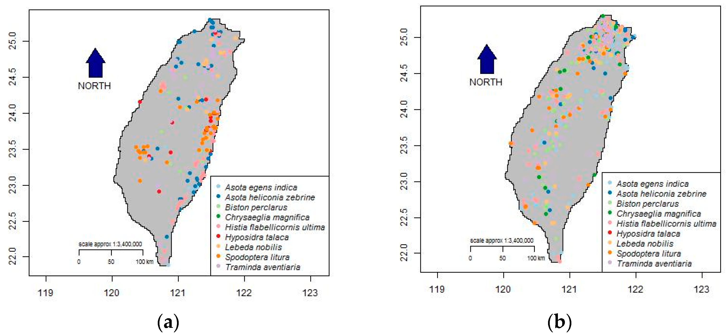
2.1. Study Area and Focal Species

Taiwan is a subtropical island with an area of 36,000 km². For this study, we selected nine moth species from the EnjoyMoths project: Asota egens indica, Asota heliconia zebrine, Biston perclarus, Chrysaeglia magnifica, Histia flabellicornis ultima, Hyposidra talaca, Lebeda nobilis, Spodoptera litura, and Traminda aventiaria (see Supplementary 2 for more details). We derived species observations and location coordinates from posts on the EnjoyMoths FB group [36]. NLP then identified FB-posted observations by species name [3].

TaiBIF [37] is the GBIF Taiwan portal specifically designed to broaden the GBIF network and increase the availability of local biodiversity data. Therefore, we used the TaiBIF portal of GBIF as the benchmark dataset in this study. We selected species with more than 15 records in the GBIF TaiBIF dataset (see Supplementary 1 for more details) to include: 37 records of A. egens indica; 103 records of A. heliconia zebrine; 29 records of B. perclarus; 39 records of C. magnifica; 58 records of H. flabellicornis ultima; 34 records of H. talaca; 21 records of L. nobilis; 33 records of S. litura, and 39 records of T. aventiaria (see Supplementary 2 for more detail) (Figure 1). We used fourteen environmental variables as focal species SDM inputs, including the first to fourth principle components of monthly precipitation (mm), the first to third principle components of monthly temperature (°C), elevation, and the Normalized Difference Vegetation Index (NDVI). We applied environmental descriptor variables to create a bio-climatic map for assessing the representation of bio-climate zones against an independent bio-climatic map of Metzger et al. [38]. We found good agreement in bioclimatic and ecosystem patterns between the created and published bio-climatic maps [3].

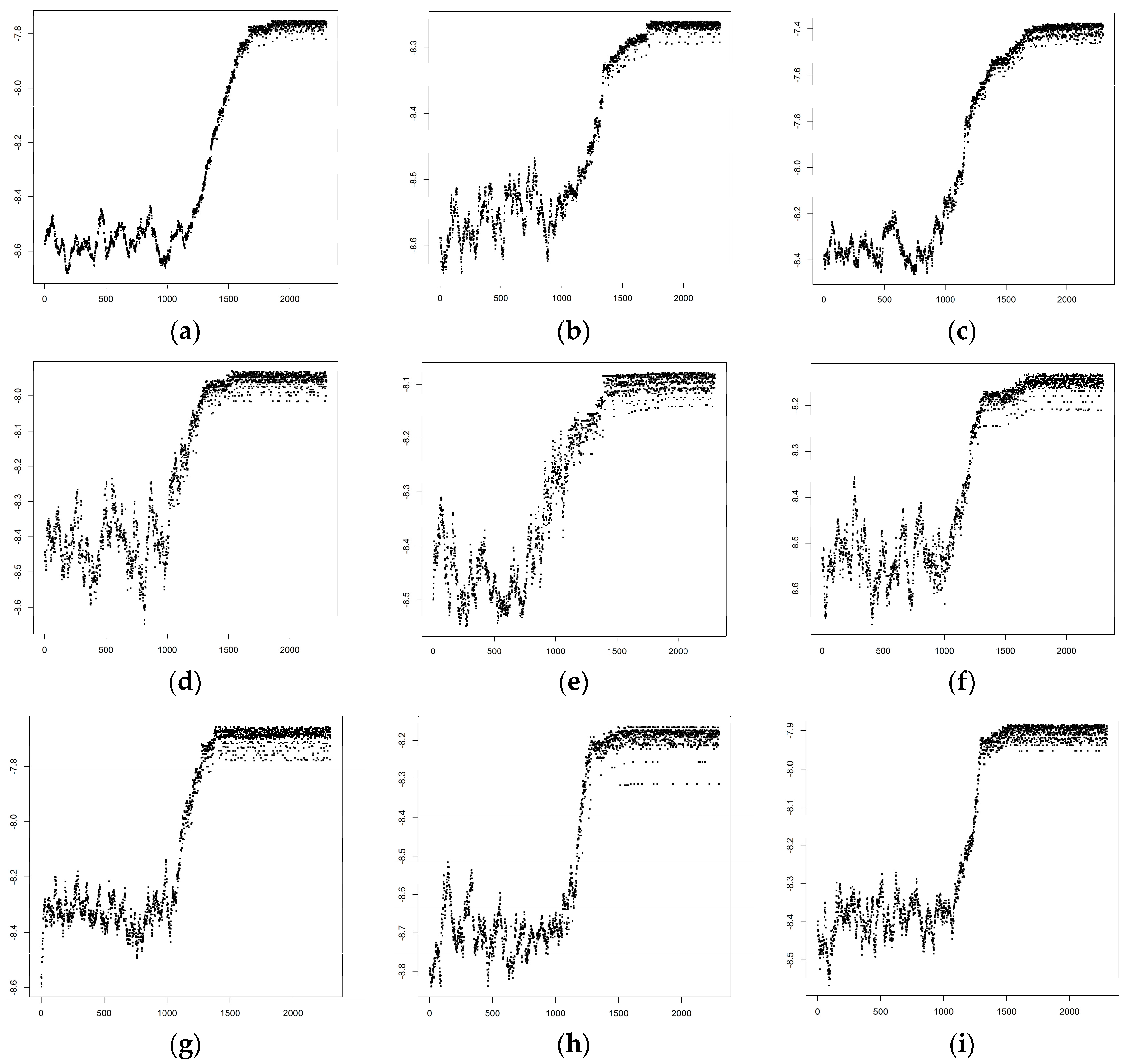
2.2. Optimal Data Filtering Method

To increase the number of available samples, we developed an optimization procedure based on a simulated annealing (SA) algorithm to integrate opportunistic data with professionally collected GBIF data. Two key parameters in the SA procedure are the cooling rates and the number of iterations during the optimization procedure. This study used three cooling rates: 0.3, 0.4, and 0.5, to obtain optimal data sets from opportunistic data. Given $N_c$ opportunistic data and $N_p$ professionally collected data, the optimization procedure aims to choose $n$ opportunistic data that can increase the average likelihood of species occurrence. We defined the average likelihood by the following equation, which is the geometric mean of the maximum entropy presence-only species distribution modeling approach:

$${\left({\displaystyle \prod }_{i=1}^{n+N_p}{q}_{\lambda }\left(x_i\right)\right)}^{\raisebox{1ex}{$1$}\!\left/ \!\raisebox{-1ex}{$\left(n+N_p\right)$}\right.}$$

(1)

where $q_{\lambda }\left(x_i\right)$ is the probability of target species presence at location $x_i$, which can be derived from the following equation based on a maximum entropy approach.

$$q_{\lambda }\left(x\right)=\frac{\exp ({{\displaystyle \sum }}_{j=1}^g{\lambda }_j·z_j\left(x\right))}{G_{\lambda }}$$

(2)

where g is the number of the environmental variables; ${\lambda }_j$ is the coefficient corresponding to driving factor $z_j$ defined by the maximum entropy model; and $G_{\lambda }$ is a normalized constant. The optimization steps are as follows:

Step 1.

Select n random samples from $N_c$ (opportunistic data).

Step 2.

Calculate the objective function, $O$, which is equal to the geometric mean of $q_{\lambda }\left(x\right)$ based on $N_{p }$ professional data and n opportunistic data.

Step 3.

Implement an annealing schedule: generate a uniform random number, $r$, between 0 and 1. If $r$< 0.5, add a sample into the n random samples from the rest of opportunistic data; otherwise, remove a sample from the n random samples at random. Calculate the objective function, $O$.

Step 4.

Calculate M = exp [−Δ$O$/T], where Δ$O$ is the change in the objective function, a comparison between the current $O$ and the last $O$, and T is the cooling rate (0–1).

Step 5.

Generate a uniformed random number (rand) in the range of 0–1. If rand < M, accept the new values; otherwise, discard the changes.

Step 6.

Repeat Steps 3–5 until either the objective function value falls beyond a given stop criterion (e.g., $O$ > a default value) or a specified number of iterations (e.g., 100,000 runs) have been completed.

2.3. Statistical Testing on Environmental Variables and HSI Similarity among Datasets

To assess the difference between the corresponding environmental variables among the five datasets ((1) GBIF; (2) FB; (3) GBIF + FB; (4) GBIF + FB_o; and (5) GBIF + FB_r), we applied the Kruskal–Wallis test. We applied the same test to the resultant SDM HSI of each dataset. When we found significant differences among datasets, we performed multiple comparisons to identify how pairs of the three datasets GBIF, FB, and FB_o, differ in terms of variable importance and HSI values. In addition, we performed correlation analysis between the average SDM benchmark outputs and the average SDM outputs.

2.4. Model Performance Evaluation and Data Bootstrapping for Uncertainty Analysis

In this study, we used four SDM types, Generalized Additive Model (GAM), Generalized Linear Model (GLM), Maximum Entropy Modeling (Maxent), and Support Vector Machine (SVM), to estimate habitat suitability distributions [39] of the focal species in addition to assessing the robustness of our data extraction method. We used the area under the curve of the receiver operating characteristic (AUC) to evaluate the performance of the above SDMs each trained by one of the five datasets: (1) GBIF; (2) FB; (3) GBIF + FB; (4) GBIF + FB_o; and (5) GBIF + FB_r. We assume that SDM performance is better when trained by the GBIF + FB_o dataset, regardless of the SDM type used. Model performance in concurrence with this assumption validates the proposed data filtering method. Additionally, to understand the variability among each dataset better, we applied a bootstrapping method to each of the five datasets and generated 1000 subsamples for each dataset consisting of 80% of the original data. We used each of the 80% subsample datasets to train the four SDM types. We then used the remaining 20% subsample datasets to test the model performances in terms of the AUC values. Boxplots illustrate the statistical distribution of AUC results. We also applied a two-sample Kolmogorov–Smirnov (K–S) test to compare differences in the 1000 AUC values between pairs of 80% subsample datasets and 20% subsample datasets of the five datasets.

We performed a principal component analysis (PCA) to evaluate the consensus between projections of 1000 realizations created by each SDM type for each data source. PCA represents the variation of independent dimensions [40], and is applicable to SDM outputs [41]. We treated the first principal component (PC1) axis as a consensus axis that reflects the general trend followed by 1000 realizations [42,43]. We evaluated the variability between 1000 realizations by calculating the proportion of explained variance from PC1 axis. When all projections are fully consistent with each other, the PC1 axis explains 100% of the variation. In contrast, if the projections were completely inconsistent, the PC1 axis explains only 0.1% of the variation (=1/1000 × 100%, where 1000 is the number of realizations) [42]. That is, a higher proportion of explained variance represents a lower variability between realizations.

3. Results

3.1. Optimized Selection of Opportunistic Data

Figures S1, S2 and Figure 2 display objective function values and average log likelihood during the optimization process under 0.3, and 0.4, and 0.5 cooling rates, respectively. As shown in Figure 2, the average log likelihood of all species converged at iteration 1500 through 1800 under a 0.5 cooling rate. The average log likelihood for nine species increased by 185.7% (0.36 to 0.93) from initial states to optimal states using the proposed approach under a 0.5 cooling rate. Moreover,

Table 1. The number of observations in GBIF, FB, FB_o, as well as the proportion of the number of observations in FB_o to the number of observations in FB.

Data Type	GBIF	FB	(FB_o)			Proportion
Species			0.3	0.4	0.5	0.3	0.4	0.5
Asota egens indica	37	170	69	60	54	41%	35%	32%
Asota heliconia zebrina	103	101	60	60	59	59%	59%	58%
Biston perclarus	29	140	58	51	43	41%	36%	31%
Chrysaeglia magnifica	39	60	23	28	23	38%	47%	38%
Histia flabellicornis ultima	58	67	10	10	11	15%	15%	16%
Hyposidra talaca	34	63	28	28	28	44%	44%	44%
Lebeda nobilis	21	63	29	28	20	46%	44%	32%
Spodoptera litura	33	59	20	20	20	34%	34%	34%
Traminda aventiaria	39	64	28	27	28	44%	42%	44%

Note: Cooling rates are 0.3, 0.4, and 0.5; Professionally collected data from Global Biodiversity Information Facility (GBIF); opportunistic data from Facebook (FB); opportunistic data from optimally selected Facebook dataset (FB_o).

shows the number of NLP extracted opportunistic GBIF, FB, FB_o, as well as the proportion of the number of observations in FB_o to the number of observations in FB for each species under 0.3, 0.4, and 0.5 cooling rates. As can be seen, by using the proposed optimal data filtering technique with a 0.5 cooling rate, the available sample data increased to a total number of 91, 162, 72, 62, 69, 62, 41, 53 and 67, for Asota egens indica, Asota heliconia zebrine, Biston perclarus, Chrysaeglia magnifica, Histia flabellicornis ultima, Hyposidra talaca, Lebeda nobilis, Spodoptera litura, and Traminda aventiaria, respectively. That is, 2.46, 1.57, 2.48, 1.59, 1.19, 1.82, 1.95, 1.61 and 1.72 times that of the original data available in the GBIF database. The average log likelihood for nine species increased from 0.29 to 0.87 under a 0.4 cooling rate, and from 0.23 to 0.71 under a 0.3 cooling rate (Figures S1 and S2).

Under a 0.5 cooling rate, the greatest proportion of data utilized from the volunteer data (58%) appears in the data filtering results of A. heliconia zebrine, while H. flabellicornis ultima shows the lowest proportion of data utilization from opportunistic data (16%).

Table 2. Observed species locations in FB red (left), GBIF blue (center), and GBIF + FB_o red/blue (right); and habitat suitability distributions based on the above-mentioned datasets for each species.

	Dataset	FB	GBIF	GBIF + FB_o
Species
Asota egens indica
Asota heliconia zebrine
Biston perclarus
Chrysaeglia magnifica
Histia flabellicornis ultima
Hyposidra talaca
Lebeda nobilis
Spodoptera litura
Traminda aventiaria

Note: Cooling rate is 0.5; Professionally collected data from Global Biodiversity Information Facility (GBIF); opportunistic data from Facebook (FB); opportunistic data from optimally selected Facebook dataset (FB_o).

maps observation locations under a 0.5 cooling rate and species distributions modeled on opportunistic data from FB, professionally collected data from GBIF, and a combination of the two. The selected opportunistic data tend to reach the highest point-densities in the north of Taiwan. Figures S3 and S4 represent optimal observation locations selected under 0.3 and 0.4 cooling rates as well as corresponding simulated species distributions (Supplementary 3).

3.2. Statistical Testing on Environmental Variables and HSI Similarity among Datasets

The average environmental variables corresponding to the three datasets, GBIF, FB, and FB_o, and the results of a Kruskal–Wallis (KW) test on the environmental variables of different datasets are shown in Table S1, as are the results of multiple comparison tests between the datasets for each environmental variable. Datasets displayed in paired combinations are those datasets that differed significantly. Significant differences of variables such as watershed, distance to city, and the third principal component of precipitation, are apparent among datasets for all species. Forest, watershed, distance to city, and the first through third principal components of temperature all demonstrated significant differences for most species. Only one variable, distance to road, was not significantly different among datasets. Table S1 also displays the average HSI values of models based on the GBIF, FB, and FB_o datasets for each species, as well as the KW p-value results between datasets and multiple comparison results for each species. All species showed significant differences between HSIs among datasets. Through multiple comparison tests, the average HSIs of FB and FB_o were shown to be significantly different for all species though the average HSIs of FB_o were greater than those of FB.

Table 3. Average correlation between species distribution models based on GBIF dataset and alternative combination dataset.

Species	FB	GBIF + FB	GBIF + FB_o	GBIF + FB_r
Asota egens indica	0.39	0.57	0.71	0.78
Asota heliconia zebrine	0.59	0.88	0.91	0.90
Biston perclarus	0.49	0.64	0.77	0.74
Chrysaeglia magnifica	0.47	0.80	0.91	0.90
Histia flabellicornis ultima	0.40	0.85	0.99	0.96
Hyposidra talaca	0.17	0.61	0.77	0.78
Lebeda nobilis	0.44	0.69	0.84	0.82
Spodoptera litura	0.19	0.62	0.83	0.82
Traminda aventiaria	0.54	0.83	0.86	0.94

Note: Opportunistic dataset from Facebook (FB); Professionally collected data from Global Biodiversity Information Facility plus opportunistic data from Facebook (GBIF+FB); Professionally collected data from Global Biodiversity Information Facility plus opportunistic data from optimally selected Facebook dataset (GBIF + FB_o); Professionally collected data from Global Biodiversity Information Facility plus opportunistic data from randomly selected Facebook dataset (GBIF + FB_r). All correlations are significant at p value < 0.05.

shows the Pearson correlation coefficients between species distributions based on the GBIF dataset and alternative combinations of various selected datasets. The SDM output averages based on the GBIF dataset and combinations of the GBIF dataset plus optimal selected or random selected opportunistic datasets are highly correlated.

3.3. Performance and Uncertainty Analysis

Table 4. Boxplots of the AUC values derived from four models (GAM, GLM, Maxent, and SVM) of five datasets (GBIF, FB, GBIF + FB, GBIF + FB_o, and GBIG + FB_r) for nine species.

SDM Type	AUC Results
GAM	Asota egens indica	Asota heliconia zebrine	Biston perclarus
	Chrysaeglia magnifica	Histia flabellicornis ultima	Hyposidra talaca
	Lebeda nobilis	Spodoptera litura	Traminda aventiaria
GLM	Asota egens indica	Asota heliconia zebrine	Biston perclarus
	Chrysaeglia magnifica	Histia flabellicornis ultima	Hyposidra talaca
	Lebeda nobilis	Spodoptera litura	Traminda aventiaria
Maxent	Asota egens indica	Asota heliconia zebrine	Biston perclarus
	Chrysaeglia magnifica	Histia flabellicornis ultima	Hyposidra talaca
	Lebeda nobilis	Spodoptera litura	Traminda aventiaria
SVM	Asota egens indica	Asota heliconia zebrine	Biston perclarus
	Chrysaeglia magnifica	Histia flabellicornis ultima	Hyposidra talaca
	Lebeda nobilis	Spodoptera litura	Traminda aventiaria

Note: Cooling rate is 0.5; Generalized Additive Model (GAM); Generalized Linear Model (GLM); Maximum Entropy Modeling (Maxent); and Support Vector Machine (SVM); Professionally collected data from Global Biodiversity Information Facility (GBIF); Opportunistic dataset from Facebook (FB); Professionally collected data from Global Biodiversity Information Facility plus opportunistic data from Facebook (GBIF + FB); Professionally collected data from Global Biodiversity Information Facility plus opportunistic data from optimally selected Facebook dataset (GBIF + FB_o); Professionally collected data from Global Biodiversity Information Facility plus opportunistic data from randomly selected Facebook dataset (GBIF + FB_r).

shows the boxplots of 1000 AUC values of four model predictions (GAM, GLM, Maxent, and SVM) based on five datasets (GBIF, FB, GBIF + FB, GBIF + FB_o, and GBIF + FB_r) under a 0.5 cooling rate. Figures S5 and S6 show the boxplots of 1000 AUC values of the model predictions with cooling rates of 0.3 and 0.4, respectively. The GBIF dataset generally led to the highest AUC variance, i.e., standard deviations, and the lowest median AUC values. In addition, the median AUCs of GBIF+FB_o are highest among those of the five datasets for Asota egens indica in all models; for Biston perclarus in GLM, Maxent, and SVM models; for Chrysaeglia magnifica in all models; for Histia flabellicornis ultima in all models; for Lebeda nobilis in GLM, Maxent, and SVM; for Spodoptera litura in GAM and Maxent; and Traminda aventiaria in all models. The median AUCs of GBIF + FB_o were higher than those of GBIF + FB_r in all cases. In other words, the SDMs based on GBIF plus FB_o datasets outperformed those based on other datasets. The two-sample K–S test results show that, for most species and datasets, the resultant AUC values were significantly different. In addition,

Table 5. Explained variation by the first PCA component of the 1000 species distributions derived from four SDMs based on five datasets under a 0.5 cooling rate.

Species	Model	Dataset
		GBIF	FB	GBIF + FB	GBIF + FB_o	GBIF + FB_r
Asota egens indica	GAM	0.90	0.97	0.98	0.97	0.90
	GLM	0.53	0.87	0.88	0.81	0.73
	Maxent	0.32	0.77	0.78	0.60	0.55
	SVM	0.68	0.82	0.82	0.87	0.72
Asota heliconia zebrina	GAM	0.95	0.98	0.98	0.98	0.96
	GLM	0.78	0.81	0.89	0.88	0.86
	Maxent	0.62	0.59	0.79	0.76	0.73
	SVM	0.81	0.85	0.84	0.85	0.81
Biston perclarus	GAM	0.91	0.98	0.98	0.97	0.91
	GLM	0.43	0.85	0.88	0.72	0.69
	Maxent	0.28	0.70	0.73	0.44	0.42
	SVM	0.72	0.82	0.80	0.83	0.73
Chrysaeglia magnifica	GAM	0.92	0.96	0.96	0.96	0.91
	GLM	0.58	0.68	0.78	0.70	0.65
	Maxent	0.30	0.41	0.57	0.43	0.38
	SVM	0.71	0.77	0.78	0.81	0.71
Histia flabellicornis ultima	GAM	0.96	0.95	0.97	0.97	0.95
	GLM	0.69	0.70	0.86	0.77	0.74
	Maxent	0.47	0.47	0.71	0.55	0.50
	SVM	0.82	0.71	0.81	0.87	0.81
Hyposidra talaca	GAM	0.90	0.95	0.95	0.95	0.90
	GLM	0.49	0.73	0.80	0.71	0.65
	Maxent	0.35	0.47	0.62	0.47	0.45
	SVM	0.64	0.82	0.80	0.81	0.73
Lebeda nobilis	GAM	0.86	0.95	0.96	0.95	0.86
	GLM	0.29	0.73	0.79	0.53	0.54
	Maxent	0.24	0.45	0.54	0.33	0.29
	SVM	0.65	0.82	0.79	0.79	0.70
Spodoptera litura	GAM	0.91	0.95	0.95	0.95	0.89
	GLM	0.35	0.68	0.71	0.59	0.53
	Maxent	0.20	0.39	0.54	0.36	0.29
	SVM	0.74	0.74	0.72	0.73	0.64
Traminda aventiaria	GAM	0.92	0.96	0.97	0.96	0.92
	GLM	0.56	0.69	0.80	0.72	0.68
	Maxent	0.31	0.40	0.60	0.41	0.40
	SVM	0.69	0.78	0.76	0.81	0.71
Average		0.62	0.75	0.81	0.75	0.69

Note: Cooling rate is 0.5; Generalized Additive Model (GAM); Generalized Linear Model (GLM); Maximum Entropy Modeling (Maxent); and Support Vector Machine (SVM); Professionally collected data from Global Biodiversity Information Facility (GBIF); Opportunistic dataset from Facebook (FB); Professionally collected data from Global Biodiversity Information Facility plus opportunistic data from Facebook (GBIF + FB); Professionally collected data from Global Biodiversity Information Facility plus opportunistic data from optimally selected Facebook dataset (GBIF + FB_o); Professionally collected data from Global Biodiversity Information Facility plus opportunistic data from randomly selected Facebook dataset (GBIF + FB_r).

shows the explained variation by the first PCA component of the 1000 species distributions derived from four SDMs based on five datasets for each species. The average explained variation under 0.5 cooling rate for GBIF, FB, GBIF + FB, GBIF + FB_o and GBIF + FB_r datasets were 0.62, 0.75, 0.81, 0.74, and 0.69, respectively. We observed similar average explained variation findings for cooling rates of 0.3 and 0.4 (Tables S2 and S3 in Supplementary).

4. Discussion

4.1. Optimal Data Filtering Procedure

Opportunistic data present advantages and challenges for sampling problems in ecology, biogeography, and conservation [10]. Although opportunistic data integrity may be compromised by a general lack of important metadata, e.g., sampling effort [4,11], suitable techniques in conjunction with reasonable assumptions can garner quality data [3,4,29]. While many opportunistic data extraction techniques have been developed and used in biological studies [3,4,10,17,33], few have considered professionally collected data based SDM outputs [32]. One recent trend uses integrated modeling techniques to utilize, or “share”, information from disparate data sources in SDMs [44] rather than strictly extracting opportunistic data. Another, more recent joint modeling method presented by Pacifici et al. [4], uses data from structured and unstructured surveys to directly inform SDMs by sharing parameters in jointly estimated likelihoods. Some approaches have even considered other criteria such as the relative competence of volunteers who upload opportunistic data [34,35]. Despite the wide range of available approaches, maximizing likelihood is the most common approach to obtain presence-only data [26]. This study used an SA approach to maximize the average likelihood of a maximum entropy presence-only species distribution model based on NLP extracted opportunistic data collected by citizen scientists and successfully identified reliable inputs with respect to the designated benchmark GBIF dataset.

More specifically, in contrast to other studies [3,4,10,11], this study proposes and validates an optimal data filtering method using SA techniques to extract samples from opportunistic data by removing unrealistic entries as identified by GBIF based SDMs. While the validation results suggest that the proposed optimal filtering method successfully selected high quality data from the opportunistic data by maximizing the likelihood function in the study cases, there are a number of caveats. For example, a basic premise of this optimization technique is that the benchmark data is relatively free of data biases, i.e., in this case the professionally collected GBIF data is free of specimen misidentification, spatial over- or underrepresentation, etc. In addition, there are a number of parameters and settings that can affect the performance and efficiency of SA. In this study, we used an exponential cooling schedule at three cooling rates, all of which Robini and Reissman [45] reported as the most successful. Theoretically, the series of iterations converge to a global optimum while the cooling rates tend to zero. In this study, by using the proposed filtering method at the 0.5 cooling rate, the average species presence probability increased by 2.2 to 10 times. Despite this, the optimal selected sample size at the 0.5 cooling rate is less than the sample sizes identified at the 0.3 and 0.4 cooling rates. The 0.5 cooling rate also produced the highest average rate of increase in the maximum likelihood value.

4.2. Uncertainty Analysis

As seen in the variation explained by the first PCA component of species HSI [42,43], uncertainty analysis revealed low uncertainty in the HSI derived from the professionally collected GBIF data plus opportunistic data from optimally selected FB dataset (GBIF + FB_o) relative to the GBIF plus opportunistic data from randomly selected FB dataset (GBIF + FB_r). Interestingly, the GBIF plus all opportunistic data from Facebook (GBIF + FB) yielded the lowest uncertainty. Given the inverse relationship between uncertainty and sample size, this could be attributable to the greater number of samples from the GBIF+FB dataset used to train the SDMs. As Buisson et al. [46] noted, assessing the uncertainty that data collection introduces into species distribution predictions is crucial, as is comparing the effects of varying dataset sizes [47].

4.3. Method Validation

Recently, numerous studies successfully used opportunistic data with various datasets in their biological mapping and species modeling [3,4,10,11,28]. In this study, we used three main validation criteria: (1) the strength of the relationship between datasets and environmental variables; (2) resultant SDM performance; and (3) uncertainty analysis. By using the proposed method to combine professionally collected GBIF data and opportunistic datasets, we obtained larger datasets that resulted in higher performing species distribution estimates with lower uncertainty than those estimates based solely on GBIF. In addition, although the GBIF + FB_o dataset contained more uncertainty than the GBIF + FB dataset, the GBIF + FB_o dataset better reflected species preferences. Our results suggest that the proposed approach improves biodiversity monitoring program data by identifying high-quality citizen science data.

Our results also clearly indicate that the proposed technique increases the number of available data by a factor of up to 2.47 times that of the original professionally collected GBIF dataset at a 0.5 cooling rate. Our approach can be used as a viable tool when combining multiple datasets of varying quality, i.e., a known high quality dataset combined with unknown quality datasets. Furthermore, our approach may be particularly useful when used in conjunction with other data integration modeling frameworks, such as that of Pacifici et al. [4], which used integrated data to handle data contamination issues. For example, the Pacifici et al. [4] correlation modeling method may enhance the randomly selected opportunistic data models in this study since the correlation model has the ability to utilize information from disparate datasets and models when parameters between various datasets cannot be shared directly, e.g., differing measurement scales or drastic differences in data quality. On the other hand, the optimally selected opportunistic data technique presented here may improve the presence only Pacifici et al. [4] shared model when the reliability of opportunistic datasets have been verified, i.e., the spatial structures and species specific environmental variables match the high-quality datasets to a high degree.

Contrary to results obtained by using NPL-extracted FB data alone [3], the optimally selected GBIF + FB_o dataset from this study tend to be located in areas that have higher GBIF-based SDM HSI. For some species, important predictive environmental variables found in GBIF and FB_o datasets exhibit more similarity with one another than with the FB datasets. For instance, for Asota egens indica, Biston perclarus, Chrysaeglia magnifica, Histia flabellicornis ultima, and Spodoptera litura, the average predictive strengths of the forest cover variable in FB_o datasets are significantly higher than those found in FB datasets. This is presumably due to the positive effects of forest cover on habitats. In contrast, FB_o datasets are less correlated with the distinct watershed area variable than the FB datasets, suggesting less bias associated with easily accessible or frequently visited recreational areas. These results indicate that suitable environmental variables should play a role in the extraction of reliable opportunistic data [10]. Our method demonstrates this when considering the SDM-identified environmental drivers during screening for potentially reliable samples.

SDMs based on the GBIF + FB_o dataset outperformed other datasets in most cases, and reflect two benefits of using the proposed data filtering technique. First, the proposed optimal data filtering technique, in most cases, i.e., species and SDM model type combinations, may enable the selection of more biologically meaningful samples as indicated by a higher performing SDM than SDMs based on GBIF + FB_r. Second, higher performing models may also be a result of larger datasets. In this study, SDMs based on GBIF + FB_o performed better than GBIF-based SDMs. That is, the results indicate that the proposed approach increases SDM sample size and performance, and decreases model uncertainty. However, similar to the results of Munson et al. [27], the GBIF only dataset-based SDM performance and the GBIF + FB_r dataset-based SDM performance had similar predictive powers in some cases. In addition to this, the GBIF-based SDM output correlation analysis revealed a high correlation with both GBIF + FB_o and GBIF + FB_r dataset-based SDM outputs. Nonetheless, the differences in spatial structure identified in the Kruskal–Wallis analysis stage of our study, as well as differences in the distribution of the AUC box-plotted analysis suggest that a data-extracting procedure is advisable. The AUC values clearly indicate lower median AUC values and higher AUC variability of models based on opportunistic data only versus models based on professionally collected data. The effectiveness of the proposed technique is also apparent when iteration durations are increased, and when the similarities between GBIF based and FB_o based model outputs are compared. The three main validation criteria used in this study: the strength of the relationship between datasets and environmental variables, resultant SDM performance, and uncertainty analysis, further support the appropriateness of the proposed filtering method in identifying high quality data. The disadvantages of non-filtered opportunistic data have also been demonstrated and include: apparent spatial biases for uninformative environmental variables; inclusion of unrealistic observational data with exceedingly low HSI values; lower SDM performance when compared to GBIF + FB_o based SDMs; and finally, higher SDM uncertainty when compared to equal sized filtered datasets. If professionally collected benchmark data are relatively unbiased, and are representative of the species of concern, the proposed technique can fill gaps in professionally collected datasets. Users should be cautious since the converse is also true, namely, if any biases exist in the benchmark dataset the proposed technique may only serve to amplify them. Despite this, the proposed optimal filtering technique has the potential to make meaningful contributions in biological conservation and policymaking since it analyzes large datasets of citizen science, validates entries, and identifies unbiased records that improve SDM predictions [3].

5. Conclusions

Opportunistic data can provide ecologists with additional samples to compensate for data gaps that may exist in the relatively small number of professionally collected, high-quality structured samples available from other sources. Our approach efficiently selected high quality, opportunistically sourced data using the proposed optimization technique with an automated NLP component, and combined this data with professionally collected GBIF data for modeling moth distributions. We used the Kruskal–Wallis test to analyze the properties of different datasets and the statistical differences between environmental variables and HSI values corresponding to benchmark data, opportunistic data, and filtered datasets. We also addressed the performance and uncertainty in SDM outputs based on different datasets by using a bootstrapping approach to generate random SDM data subsets. Our proposed data filtering method is a tool for filling current data gaps and improving biodiversity monitoring or biological conservation initiatives. By referencing reliable benchmark data, the proposed data extraction technique can garner valuable data from large unstructured datasets, thereby improving ecological data quality and quantity.

References

1. Isaac, N.J.B.; van Strien, A.J.; August, T.A.; Zeeuw, M.P.D.; Roy, D.B. Statistics for citizen science: Extracting signals of change from noisy ecological data. Methods Ecol. Evol. 2014, 5, 1052–1060. [Google Scholar] [CrossRef]
2. Worthington, J.P.; Silvertown, J.; Cook, L.; Cameron, R.; Dodd, M.; Greenwood, R.M.; McConway, K.; Skelton, P. Evolution megalab: A case study in citizen science methods. Methods Ecol. Evol. 2012, 3, 303–309. [Google Scholar] [CrossRef]
3. Lin, Y.-P.; Deng, D.; Lin, W.-C.; Lemmens, R.; Crossm, N.D.; Henle, K.; Schmeller, D.S. Uncertainty analysis of crowd-sourced and professionally collected field data used in species distribution models of taiwanese moths. Biol. Conserv. 2015, 181, 102–110. [Google Scholar] [CrossRef]
4. Pacifici, K.; Reich, B.J.; Miller, D.A.W.; Gardner, B.; Stauffer, G.; Singh, S.; McKerrow, A.; Collazo, J.A. Integrating multiple data sources in species distribution modeling: A framework for data fusion. Ecology 2017, 98, 840–850. [Google Scholar] [CrossRef] [PubMed]
5. Silvertown, J. A new dawn for citizen science. Trends Ecol. Evol. 2009, 24, 467–471. [Google Scholar] [CrossRef] [PubMed]
6. Dickinson, J.L.; Zuckerberg, B.; Bonter, D.N. Citizen science as an ecological research tool: Challenges and benefits. Annu. Rev. Ecol. Evol. Syst. 2010, 41, 149–172. [Google Scholar] [CrossRef]
7. Newman, G.; Zimmerman, D.; Crall, A.; Laituri, M.; Graham, J.; Stapel, L. User-friendly web mapping: Lessons from a citizen science website. Int. J. Geogr. Inf. Sci. 2010, 24, 1815–1869. [Google Scholar] [CrossRef]
8. Jackson, M.M.; Gergel, S.E.; Martin, K. Citizen science and field survey observations provide comparable results for mapping vancouver island white-tailed ptarmigan (lagopus leucura saxatilis) distributions. Biol. Conserv. 2015, 181, 162–172. [Google Scholar] [CrossRef]
9. Ratnieks, F.L.W.; Schrell, F.; Sheppard, R.C.; Brown, E.; Bristow, O.E.; Garbuzov, M. Data reliability in citizen science: Learning curve and the effects of training method, volunteer background and experience on identification accuracy of insects visiting ivy flowers. Methods Ecol. Evol. 2016, 7, 1226–1235. [Google Scholar] [CrossRef]
10. Bried, J.T.; Siepielski, A.M. Opportunistic data reveal widespread species turnover in enallagma damselflies at biogeographical scales. Ecography 2017. [Google Scholar] [CrossRef]
11. Louvrier, J.; Duchamp, C.; Lauret, V.; Marboutin, E.; Cubaynes, S.; Choquet, R.; Miquel, C.; Gimenez, O. Mapping and explaining wolf recolonization in france using dynamic occupancy models and opportunistic data. Ecography 2017. [Google Scholar] [CrossRef]
12. Sullivan, B.L.; Phillips, T.; Dayer, A.A.; Wood, C.L.; Farnsworth, A.; Iliff, M.J.; Davies, I.J.; Wiggins, A.; Fink, D.; Hochachka, W.M.; et al. Using open access observational data for conservation action: A case study for birds. Biol. Conserv. 2017, 208. [Google Scholar] [CrossRef]
13. eBird. Available online: http://eBird.org (accessed on 29 September 2017).
14. Stafford, R.; Hart, A.G.; Collins, L.; Kirkhope, C.L.; Williams, R.L.; Rees, S.G.; Lloyd, J.R.; Goodenough, A.E. Eu-social science: The role of internet social networks in the collection of bee biodiversity data. PLoS ONE 2010, 5, e14381. [Google Scholar] [CrossRef] [PubMed] [Green Version]
15. Aanensen, D.M.; Huntley, D.M.; Feil, E.J.; al-Own, F.; Spratt, B.G. Epicollect: Linking smartphones to web applications for epidemiology, ecology and community data collection. PLoS ONE 2009, 4, e6968. [Google Scholar] [CrossRef] [PubMed]
16. Delaney, D.G.; Sperling, C.D.; Adams, C.S.; Leung, B. Marine invasive species: Validation of citizen science and implications for national monitoring networks. Biol. Invasions 2008, 10, 117–128. [Google Scholar] [CrossRef]
17. Roy, H.E.; Adriaens, T.; Isaac, N.J.B.; Kenis, M.; Onkelinx, T.; Martin, G.S.; Brown, P.M.J.; Hautier, L.; Poland, R.; Roy, D.B.; et al. Invasive alien predator causes rapid declines of native european ladybirds. Divers. Distrib. 2012, 18, 717–725. [Google Scholar] [CrossRef]
18. Zapponi, L.; Cini, A.; Bardiani, M.; Hardersen, S.; Maura, M.; Maurizi, E.; Zan, L.R.D.; Audisio, P.; Bologna, M.A.; Carpaneto, G.M.; et al. Citizen science data as an efficient tool for mapping protected saproxylic beetles. Biol. Conserv. 2017, 208, 139–145. [Google Scholar] [CrossRef]
19. Geldmann, J.; Heilmann-Clausen, J.; Holm, T.E.; Levinsky, I.; Markussen, B.; Olsen, K.; Rahbek, C.; Tøttrup, A.P. What determines spatial bias in citizen science? Exploring four recording schemes with different proficiency requirements. Divers. Distrib. 2016, 22, 1139–1149. [Google Scholar] [CrossRef]
20. Guillera-Arroita, G. Modelling of species distributions, range dynamics and communities under imperfect detection: Advances, challenges and opportunities. Ecography 2017, 40, 281–295. [Google Scholar] [CrossRef]
21. Vantieghem, P.; Maes, D.; Kaiser, A.; Merckx, T. Quality of citizen science data and its consequences for the conservation of skipper butterflies (hesperiidae) in flanders (northern belgium). J. Insect Conserv. 2017, 21, 451–463. [Google Scholar] [CrossRef]
22. Bonney, R.; Shirk, J.L.; Phillips, T.B.; Wiggins, A.; Ballard, H.L.; Miller-Rushing, A.J.; Parrish, J.K. Citizen science. Next steps for citizen science. Science 2014, 343, 1436–1437. [Google Scholar] [CrossRef] [PubMed]
23. Genet, K.S.; Sargent, L.G. Evaluation of methods and data quality from a volunteer-based amphibian call survey. Wildl. Soc. Bull. 2003, 31, 703–714. [Google Scholar]
24. Kamp, J.; Oppel, S.; Heldbjerg, H.; Nyegaard, T.; Donald, P.F. Unstructured citizen science data fail to detect long-term population declines of common birds in denmark. Divers. Distrib. 2016, 22, 1024–1035. [Google Scholar] [CrossRef]
25. Elith, J.; Graham, C.H.; Anderson, R.P.; Dudík, M.; Ferrier, S.; Guisan, A.; Hijmans, R.J.; Huettmann, F.; Leathwick, J.R.; Lehmann, A.; et al. Novel methods improve prediction of species’ distributions from occurrence data. Ecography 2006, 29, 129–151. [Google Scholar] [CrossRef]
26. Fithian, W.; Elith, J.; Hastie, T.; Keith, D.A. Bias correction in species distribution models: Pooling survey and collection data for multiple species. Methods Ecol. Evol. 2015, 6, 424–438. [Google Scholar] [CrossRef] [PubMed]
27. Munson, M.A.; Caruana, R.; Fink, D.; Hochachka, W.M.; Iliff, M.; Rosenberg, K.V.; Sheldon, D.; Sullivan, B.L.; Wood, C.; Kelling, S. A method for measuring the relative information content of data from different monitoring protocols. Methods Ecol. Evol. 2010, 1, 263–273. [Google Scholar] [CrossRef]
28. Van Strien, A.J.; van Swaay, C.A.M.; Termaat, T. Opportunistic citizen science data of animal species produce reliable estimates of distribution trends if analysed with occupancy models. J. Appl. Ecol. 2013, 50, 1450–1458. [Google Scholar] [CrossRef]
29. Kosmala, M.; Wiggins, A.; Swanson, A.; Simmons, B. Assessing data quality in citizen science. Front. Ecol. Environ. 2016, 14, 551–560. [Google Scholar] [CrossRef]
30. Sullivan, B.L.; Aycrigg, J.L.; Barry, J.H.; Bonney, R.E.; Bruns, N.; Cooper, C.B.; Damoulas, T.; Dhondt, A.A.; Dietterich, T.; Farnsworth, A.; et al. The ebird enterprise: An integrated approach to development and application of citizen science. Biol. Conserv. 2014, 169, 31–40. [Google Scholar] [CrossRef]
31. Theobald, E.J.; Ettinger, A.K.; Burgess, H.K.; DeBey, L.B.; Schmidt, N.R.; Froehlich, H.E.; Wagner, C.; HilleRisLambers, J.; Tewksbury, J.; Harsch, M.A.; et al. Global change and local solutions: Tapping the unrealized potential of citizen science for biodiversity research. Biol. Conserv. 2015, 181, 236–244. [Google Scholar] [CrossRef]
32. Jetz, W.; McPherson, J.M.; Guralnick, R.P. Integrating biodiversity distribution knowledge: Toward a global map of life. Trends Ecol. Evol. 2012, 27, 151–159. [Google Scholar] [CrossRef] [PubMed]
33. Maes, D.; Vanreusel, W.; Jacobs, I.; Berwaerts, K.; Dyck, H. Applying iucn red list criteria at a small regional level: A test case with butterflies in flanders (north belgium). Biol. Conserv. 2012, 145, 258–266. [Google Scholar] [CrossRef]
34. Yu, J.; Wong, W.-K.; Hutchinson, R.A. Modeling experts and novices in citizen science data for species distribution modeling. In Proceedings of the 2010 IEEE International Conference on Data Mining, Sydney, Australia, 13–17 December 2010; pp. 1157–1162. [Google Scholar]
35. Yu, J.; Kelling, S.; Gerbracht, J.; Wong, W.-K. Automated data verification in a large-scale citizen science project: A case study. In Proceedings of the 2012 IEEE 8th International Conference on E-Science, Chicago, IL, USA, 8–12 October 2012; pp. 1–8. [Google Scholar]
36. Enjoymoths FB Group. Available online: https://www.facebook.com/groups/EnjoyMoths2/ (accessed on 29 September 2017).
37. Taiwan Biodiversity Information Facility. Available online: http://taibif.tw/en (accessed on 29 September 2017).
38. Metzger, M.J.; Bunce, R.G.H.; Jongman, R.H.G.; Sayre, R.; Trabucco, A.; Zomer, R. A high-resolution bioclimate map of the world: A unifying framework for global biodiversity research and monitoring. Glob. Ecol. Biogeogr. 2013, 22, 630–638. [Google Scholar] [CrossRef]
39. Guisan, A.; Thuiller, W. Predicting species distribution: Offering more than simple habitat models. Ecol. Lett. 2005, 8, 993–1009. [Google Scholar] [CrossRef]
40. Peterson, A.T.; Papeş, M.; Eaton, M. Transferability and model evaluation in ecological niche modeling: A comparison of garp and maxent. Ecography 2007, 30, 550–560. [Google Scholar] [CrossRef]
41. Naimi, B.; Araújo, M.B. Sdm: A reproducible and extensible r platform for species distribution modelling. Ecography 2016, 39, 368–375. [Google Scholar] [CrossRef]
42. Thuiller, W. Patterns and uncertainties of species’ range shifts under climate change. Glob. Chang. Biol. 2004, 10, 2020–2027. [Google Scholar] [CrossRef]
43. Grenouillet, G.; Buisson, L.; Casajus, N.; Lek, S. Ensemble modelling of species distribution: The effects of geographical and environmental ranges. Ecography 2011, 34, 9–17. [Google Scholar] [CrossRef]
44. Dorazio, R.M. Accounting for imperfect detection and survey bias in statistical analysis of presence-only data. Glob. Ecol. Biogeogr. 2014, 23, 1472–1484. [Google Scholar] [CrossRef]
45. Robini, M.C.; Reissman, P.-J. From simulated annealing to stochastic continuation: A new trend in combinatorial optimization. J. Glob. Optim. 2013, 56, 185–215. [Google Scholar] [CrossRef]
46. Buisson, L.; Thuiller, W.; Casajus, N.; Lek, S.; Grenouillet, G. Uncertainty in ensemble forecasting of species distribution. Glob. Chang. Biol. 2009, 16, 1145–1157. [Google Scholar] [CrossRef]
47. Barry, S.; Elith, J. Error and uncertainty in habitat models. J. Appl. Ecol. 2006, 43, 413–423. [Google Scholar] [CrossRef]
Figure 1. Focal species distribution from: (a) GBIF TaiBIF; and (b) EnjoyMoth Facebook data. Note: Global Biodiversity Information (GBIF) Taiwan portal dataset (TaiBIF).
Environments 04 00081 g001
Figure 2. Objective function values or geometric mean of likelihood of all included samples, demonstrated (Y axis) versus the iterations (X axis) under a 0.5 cooling rate for: (a) Asota egens indica; (b) Asota heliconia zebrine; (c) Biston perclarus; (d) Chrysaeglia magnifica; (e) Histia flabellicornis ultima; (f) Hyposidra talaca; (g) Lebeda nobilis; (h) Spodoptera litura; and (i) Traminda aventiaria.
Environments 04 00081 g002