Comparative Simulation of Various Agricultural Land Use Practices for Analysis of Impacts on Environments

Abstract

Current intensification and changes in agricultural land use practices increase environmental impact that can be reduced by bridging the gap between socio-economic demands and scientific justification of sustainable agricultural land use. This can be achieved by replacing the goal of maximum crop yields with the goal of minimal environmental impact. This paper presents results of integrated crop simulation system development for analysis of alternative planning strategies in agricultural land use, with focus on the crop rotation influence on environmental sustainability. The effective tools used in analysis include (1) long-term analysis of changes in agricultural land using a dynamic crop model with daily time step; (2) justification of arbitrary crop rotation scheme of different agro-technologies and sparing measures; and (3) analysis of modern farming management methods using model-oriented approach. The results of study also include estimation of two alternative practices of crop harvesting including remaining or removing whole crop residues from the agricultural field and their influence on basic parameters of soil fertility. In addition, we analyzed comparative efficiency of different agricultural measures neglecting the negative influence of possible climate changes in long-term consequences. Corresponding efficiency rating is the following: organic fertilizer, green manure legume sparing harvesting, winter catch crop, and rotation scheme.

1. Introduction

The modern progress in the development of agricultural crop models has led to a new understanding of different processes taking place in the soil-plant-atmosphere system and its influence on the environment [1,2]. AGROTOOL is the typical eco-physiological process-oriented dynamic crop model to support decision making in agricultural land use [3] that was developed to estimate the agro-meteorological state of crops, to forecast crop growth, and to analyze irrigation, sowing, harvesting, fertilization management, and environmental impact [4]. An imitation algorithm of plant growth in AGROTOOL is invariant. Therefore, the model AGROTOOL is a generic crop simulator, which is applicable for modeling a variety of crops such as barley, winter and spring wheat, alfalfa, maize, and so on [3,5].

Sustainable fertility maintenance of agricultural landscapes during their active usage is one of the widely discussed problems in environmental agricultural science [5,6]. The importance of mentioned problem has recently redoubled due to essential changes in agricultural land use worldwide [7]. For example, modern agricultural energy-oriented land use needs scientific modeling support in many aspects, such as justification of the cultivation crops, justification of crop rotation scheme, justification of spatial allocation of the crops, etc. [8]. The main problem in agricultural land use change and its impact on environment is to overcome the contradiction between economic requests from society and needs in sustainable development of agro-landscapes [9]. Therefore, in recent years, agricultural science encouraged researches to pay more attention to the environmental sustainability of the agro-landscapes instead of reaching their maximum productivity [2,7,10,11].

Consequently, an adequate justification for the new adaptive-landscape, resource-saving agricultural technologies and farming systems requires a shift from the widely used regression (statistically based) models to process-based dynamic simulation models of agro-ecosystems [12]. In this case, the main challenge is to make the process-based dynamic crop model the core of a new generation of intelligent decision support systems in agriculture [13]. In these systems, simulation crop models of agro-ecosystems is an effective tool for environmental analysis and forecasting [14]. The advantages of dynamic crop models over static statistical based models include [15] wider range of options in relation to a variety of environmental data, increase in the adequacy and accuracy of modeling results due to accounting for a broader range of factors, a broad range of the state variables (growth phase, productivity, yield, fertility) of an agricultural ecosystem analyzed during modeling; obtaining results according to external variable conditions (i.e., weather), and a decline in the degree of uncertainties in modeling results.

The above mentioned advantages of dynamic crop models are the rationale for their wide application to agro-ecosystem analysis and crop growing management within a particular growing season (time scale is small) [16,17]. However, the use of models for long-term planning is still in its infancy [18]. This is due to technical limitations in computer power and memory. Currently, due to the progress in development of computer and information technologies, the most significant technical limitations have been overcome. Therefore, use of crop models have become important in mid-term and long-term agricultural forecasting [2,11,19].

The solution of this problem requires adaptation of crop models and corresponding software [20]. The main problem is description and management of the changes in parameters of an agro-ecosystem state during the long-term crop rotation [4,7]. The solution involves following specific requirements [11]:

• Universal character of the simulation algorithm, e.g., structural identity of the models for different crop/species, climate-soil conditions and crop growth technologies.
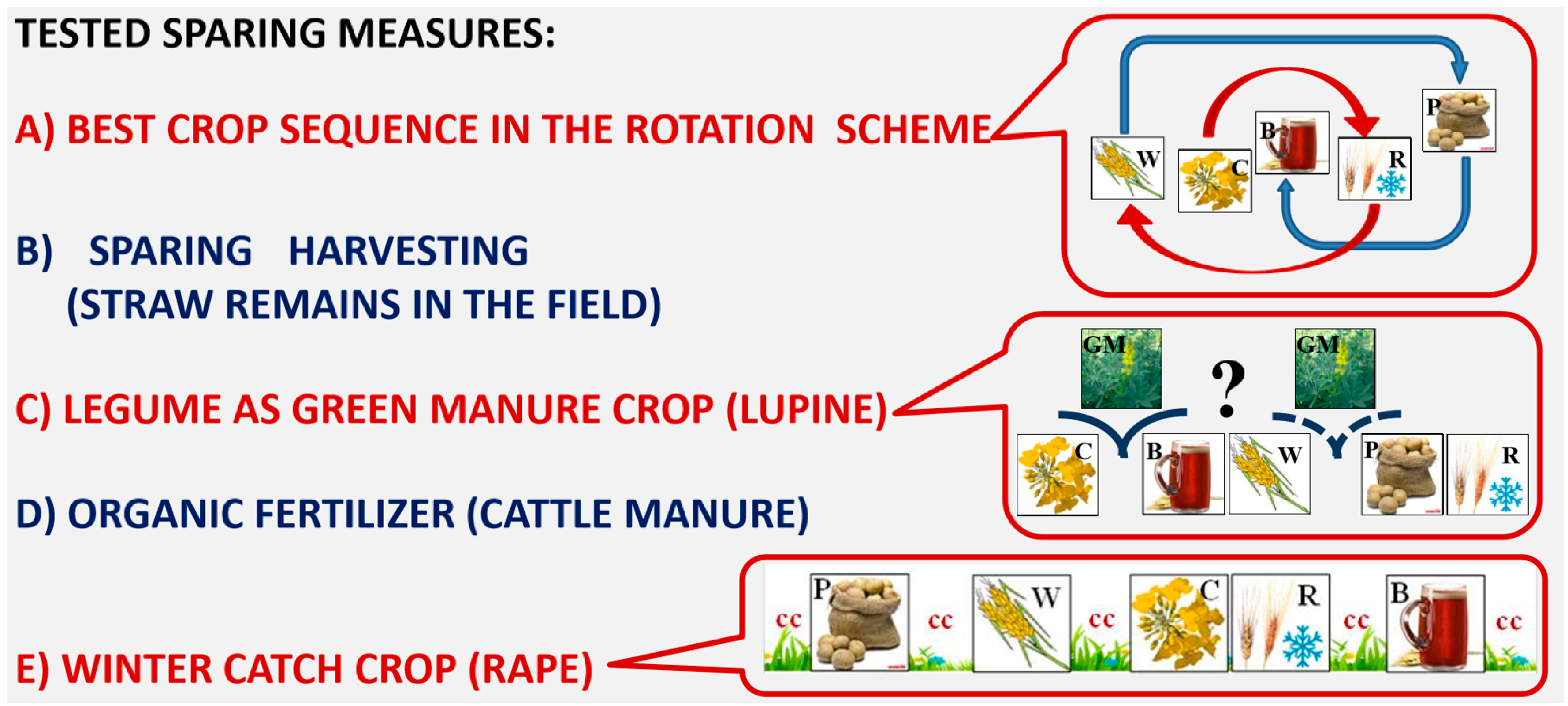
• Comprehensive sequence analysis. The model should consider the influence of crop/species predecessors in all essential aspects such as symbiotic nitrogen fixation by legumes, changes in the agro-chemical and the agro-physical soil properties under tillage, decomposition of crop residues, etc. [21].
• Wintering imitation. The model during simulation should take into account abiotic processes in the agro-ecosystem, such as snowfall, soil frost penetration and thawing, snow melting in off-seasons period, etc.
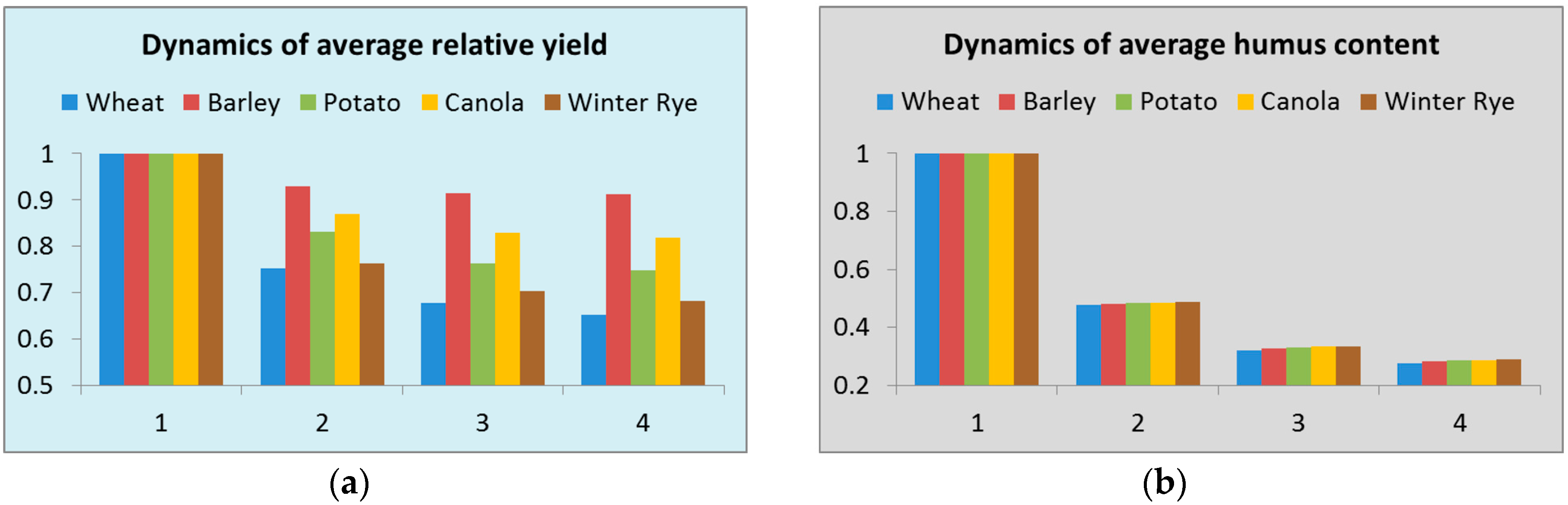
• Ecological/environmental orientation. The modeling capacities should include not only yield estimation but the forecast of dynamics of various agro-ecosystem sustainability parameters such as (1) energy-matter balance in the agro-landscape including emission of greenhouse gases; (2) nutrition substance transfer to water body; (3) soil carbon sequestration; and (4) humus content (fertility indexes).

The solution became possible with development of ecologically oriented comprehensive crop models and special software environments for a cyclical scheme of model computation that takes into account crop rotation [3,4,5,11,22,23]. This provides an opportunity to analyze long-term trends of indicators of soil fertility and other environmental parameters of the agro-landscapes. The above list of requirements for “model-oriented” decision-making system for support sustainable agriculture seems to be too strict. However, several prototypes of such systems have been developed. One example is DSSAT. This model is the leading solution for crop modeling in the USA. DSSAT includes special option for crop rotation analysis that estimate environmental impacts and economic risks taking into account fertilizer management, irrigation, soil carbon sequestration, climate changes, and precision agriculture management [24]. Several examples of successful DSSAT applications for optimization of combination of crop residue and crop rotation analysis [25,26], and analyses of nitrogen application rate for sustainable crop production [27] are also well known. In European Union one of the most known solutions for model-based analysis incorporating mid-term planning at a farm scale is LandСаRе-DSS developed by the Leibniz Center of Agro-Landscape Research [6,28].

Methods and versatile technical solutions proposed for mid- and long-term forecasting of productivity of agricultural crops for the areas with various spatial coverage (from all over the country to a single field) will bridge above mentioned gaps. Also, the proposed approaches form a common methodology of impact analysis in various agricultural land use practices [3,4,5,11,29]. The efforts for development and improvement of the integrated software environment for crop models APEX (Automation of Polivariant Experiments) [11] are presented. The improved system was used for the analysis and improvement of alternative medium-term planning strategies on agro-landscape management, taking into account the type of crop rotation influence on environmental sustainability. Two tasks have been analyzed. The first task was to estimate two alternative practices of crop harvesting and their influence on basic indices of soil fertility. These alternative practices included leaving or removing all crop residues from the agricultural fields during harvesting. The second task was to analyze the comparative efficiency of different agricultural measures neglecting the negative influence of possible climate changes in long-term consequences. Instead of purely theoretical case study described above (the single culture, the same weather realization, etc.), this computational experiment takes into account many factors and becomes close to a real situation.

2. Materials and Methods

2.1. Model AGROTOOL

The simulation algorithm of AGROTOOL, as with any other dynamical crop model, can be written in the form of recurrent discrete expression.

x(k + 1) = f(x(k), a, w(k), u(k)),  x(0) = x₀, k = 0,1...T,

(1)

where x—vector of dynamic state variables; a—vector of constant parameters; u—vector controlled external impacts (agricultural treatments); w—vector uncontrollable external impacts (weather); k—the time step for the model (time step is equal to one day), f—the evolution operator (a logical essence of the simulation algorithm), x₀—vector of initial state, T—last step of simulation [3].

The crop model AGROTOOL v.3.5. (AFI, St.Petersburg, Russia) is the third production level model (Figure 1) according to de Wit’s classification. This means that availability of water and nitrogen are the main limiting factors reducing the potential photosynthesis-based productivity [30,31].

Process description involved in AGROTOOL covers several modeling domains in crop simulation approach (

Table 1. Processes involved in AGROTOOL and the principal approaches of their implementation.

Modeling Domain	Approach
Leaf Area Development & Light Interception	Detailed model based on Monsi-Saeki approach
Light Utilization	Original model of photosynthesis as well dark metabolism
Yield Formation	Y(PRT)—Partitioning during reproductive stages
Crop Phenology	f(Temperature, Water)
Root Distribution over Depth	Exponential, based on water availability
Stresses Involved	W, N
Water Dynamics	Richards equation in 10-layer soil profile
Evapotranspiration	Modified FAO56 approach
Soil CN-model	C-N transfer and interaction in plant and soil, 5 organic pools

).

There are several modules in the crop model AGROTOOL software that are independent, scalable, replaceable, interacting at every model time step:

(1) The agrometeorological module. This module provides a connection to the database with meteorological data about daily weather data including air humidity, minimum and maximum temperature, solar radiation characteristics and precipitation which are need for crop modeling.

(2) The module of radiation and photosynthesis. This module provides calculations of the daily solar radiation sum that is intercepted and absorbed by crops, as well as the corresponding daily sum of assimilates, which are accumulated due to photosynthesis and dark metabolism.

(3) The module of turbulent gas exchange. This module provides calculations of the profile of the wind speed above and inside the crops, and corresponding aerodynamic resistance for fluxes of heat and water vapor as well as carbon dioxide.

(4) The module of soil water dynamics. This module provides calculations of the soil moisture balance using 10-layer presentation of the one-meter till. The balance is calculated taking into account precipitation, water evaporation from soil, transpiration of crops, water transfer within the soil layers, and percolation. Calculation also includes main hydro-physical soil constants such as maximum hydroscopy, field capacity and saturation capacity [32,33].

(5) The module of plant growth and development. This module includes some specific functions related to “growth distribution”, which is intended for the estimation of the dry matter increase for different parts of crops. Special concept was developed for definition of the shoot-root balanced growth during all stages of crops vegetative development. Also, the “physiological time” is calculated as the sum of effective temperatures; this parameter is corrected according to the effect of crop’s water-stress.

(6) The module of nitrogen transfers and transformations in soil. This module is created for modelling of main processes describing the soil nitrogen status: ammonification, litter humification, denitrification/nitrification, root nitrogen uptake, symbiotic nitrogen fixation by legumes, etc.

(7) The module for control of principal agronomical tillage. This module provides model control of following tillage: sowing, nitrogen fertilizing and top dressing, irrigation, and harvesting. All these agronomical impacts can be imitated both in declarative and reactive mode. This means usage of predetermined dates and rates of actions, or formal rules based on the feedback of values of internal variables of the model respectively.

AGROTOOL has a successful story of verification in Russia [3,4,5,11].

• Leningrad region (North-West of Russia): Spring barley, summer wheat, winter rye, oat, potato, perennial grasses.
• Saratov region (middle Volga): Summer wheat in long-term water stress field experiment.
• Krasnodar region (South-West of Russia): Summer wheat, maize.
• Altai region (West Siberia): Alfalfa, summer wheat.
• Kaliningrad region (The most Western region of Russia): Summer wheat, perennial grasses.
• Tver’ region (Central region of Russia): Summer wheat, spring barley, perennial grasses, rape, potato, oat. Landscape field has been tested as well.

Also, AGROTOOL has been successfully verified in Muncheberg & Badlauchstadt (Germany) for summer wheat, spring barley, and sugar beet.

2.2. Multivariate Analysis in “APEX”: Integrated Software Environment for Crop Models

Automation of Polivariant Experiments (APEX) is an integrated software environment for crop models developed in Laboratory of Agroecosystem Simulation (Agrophysical Research Institute, Saint-Petersburg). APEX provides setting, execution and analysis of multi-factor computer experiments using arbitrary crop simulation models. There are two basic features in APEX for multivariate analysis. APEX can be used as versatile repository of external descriptors of the dynamic crop models. Special dialog inside APEX allows users to register their own crop models. Also, the APEX interface includes user-friendly module for polyvariant/multyvariant analysis of modeling results. Inside APEX, a user can design multivariate case study, execute the model in batch mode, and finally execute advanced functions of statistical analysis for obtained results. APEX is the advanced software providing information support, planning, and analysis of multivariate computer experiments with crop models.

Model polyvariant analysis or computer experiment procedure in APEX is based on three principal concepts. They are “Factor level”, “Scenario”, and “Project”. “Factor level” is a dataset of one or many data tables related to one of predefined factors. “Scenario” is the tuple of the links to the levels of key factors required for a single model run. These key factors are the following: “soil”, “culture”, “location”, “initial state”, “technology”, and “weather”. During the model registration APEX allows users to define the structure of variables and parameters for the specific model and to generate a list of tables and their fields and an array of metadata. Finally, the “Project” contains the list of output scenarios (Figure 2).

There are several ways to manage data in the “Factor level” block. User can enter them manually, import from different external sources, apply stochastic generators (weather generator, for instance), propagation of existing level by means of varying one or several characteristics on a grid of values.

The project in APEX can be calculated and modified at any time. The model executes current scenario with input data sets and saves obtained results in APEX database. After project calculations are finished the results can be analyzed using statistical tools inside the system. In APEX, the strict specification of possible factors provides a clear understanding of the nature of compared scenarios. This approach provides wide opportunities for semantically rich analysis of the calculation results. The usage of APEX coupled with the crop model AGROTOOL allows us to create a real information decision support for solving typical problems of agro-ecological management.

Typical problems that might require multivariate analysis methodology are presented in

Table 2. Challenges for multivariant analysis.

Problem	Source of Multivariance
Sensitivity analysis and parametric identification	Parameter value variability
Statistical analysis and productivity assessment	Actual weather
Climate change influence on crop productivity	Future weather scenarios
Optimization of agrotechnologies	Variants (dates and rates) of technological treatments
Operative information support of field experiments	Variants of technological treatments and future weather to the end of vegetation period
Precision agriculture and GIS integration	Spatial heterogeneity of agricultural field
Long-term analysis of crop rotation	Fields, seasons, and cultures of rotation under investigation

.

2.3. Long-Term Analysis of Different Crop Rotations

Certain challenges and requirements for use in dynamic crop models for crop rotation analysis include:

• Improving the accuracy and adequacy of simulation in multifactor settings;
• Multivariable computation (e.g., weather vs. climate);
• Statistical interpretation of simulation results and risk analysis;
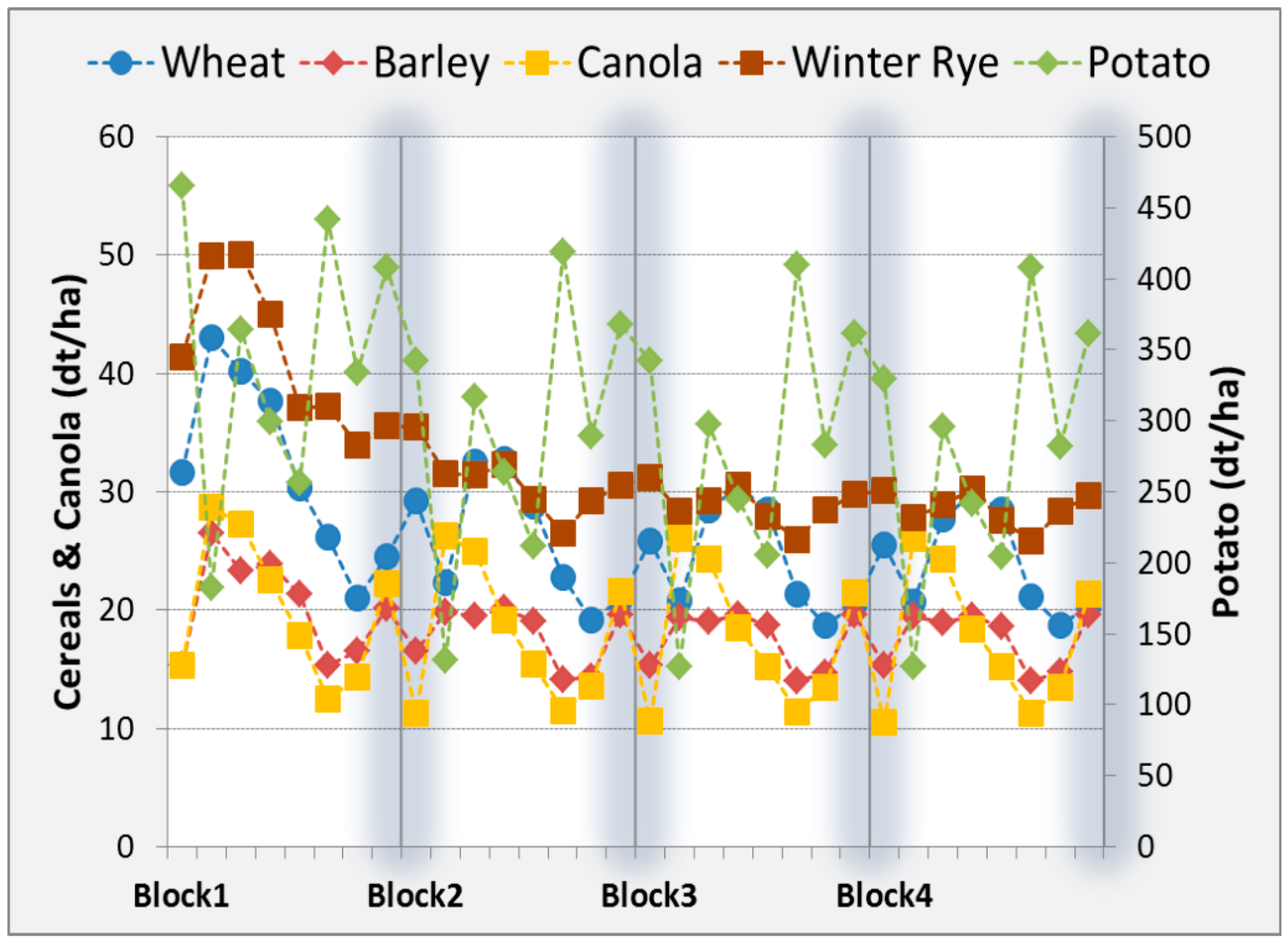
• Large number of model controlled/monitored characteristics such as productivity, physiology, ecology, fertility, etc.;
• Management of model uncertainties;
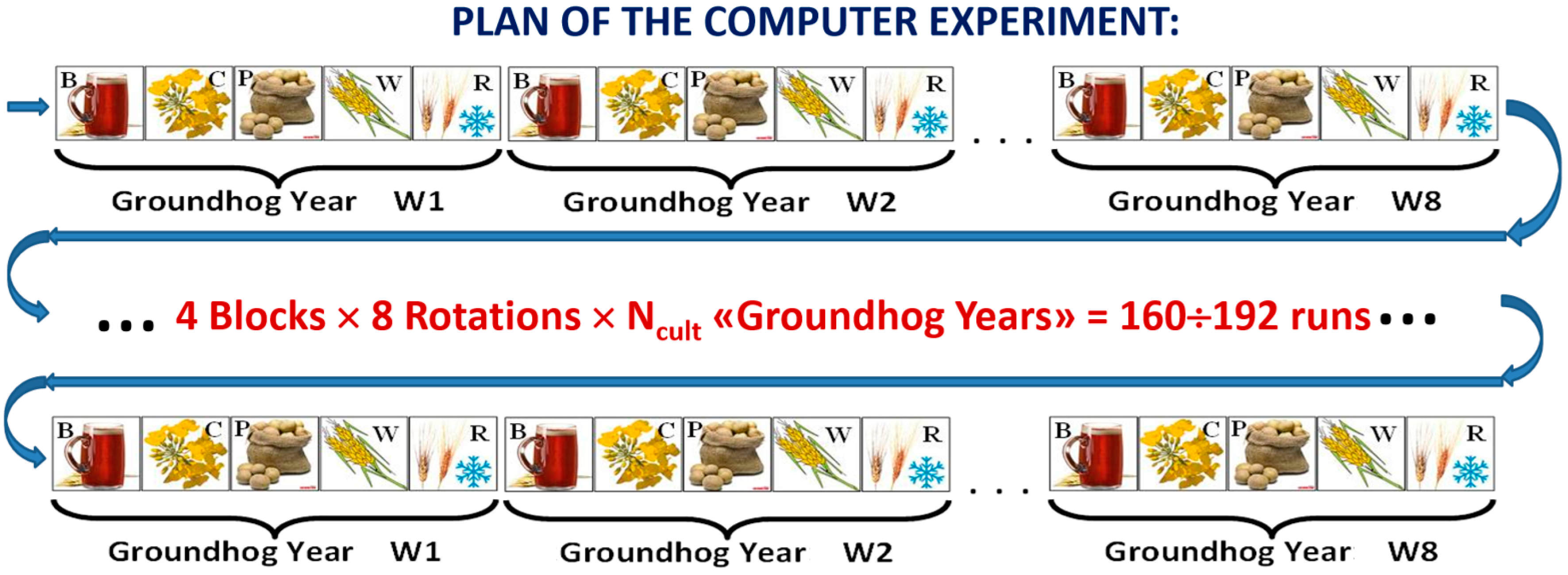
• Simulation of several consequent vegetation periods according to a chosen rotation scheme;
• The model must simulate different cultures and take into consideration agroecosystem dynamics during non-growing season (wintering);
• The runtime framework must support the calculation of scenarios in a predetermined sequence and the transfer of data from the previous scenario to the next one.

The calculation of crop rotations in APEX required the following additional functionality that was developed in this study:

• mechanism for the direct specification of the execution sequence inside scenarios in the APEX project and to specify “boundary condition” scenarios, defining the beginning of the new crop rotation block for a particular agricultural field;
• An adequate interface/method for the transfer of the results of the previous scenario into the next scenario as initial state. This method must take into account previous crop on agricultural field in the procedure of the metadata specification describing the connected model.

Analysis of the success of the above mentioned requirements to APEX and AGROTOOL for mid-term planning in land use is presented in

Table 3. APEX and AGROTOOL for crop rotation analysis.

Requirement	Current State
Crop Model:	AGROTOOL:
Generic simulator	Versatile algorithm for all maintained cultures. Calibrated models for cereals (summer and winter wheat, winter rye, barley, oats), maize, potato, root vegetables, annual and perennial forages, legumes.
Uninterrupted runs	Separated calculation of litter and root residues in the module of carbon-nitrogen transfer and transformation in soil. Sub-model of symbiotic nitrogen fixation and nodule nitrogen dynamics.
“Wintering”	Snow coverage and snow melting sub-models.
Simulation infrastructure:	APEX (Automation of Polivariant Experiments):
Multiple running	Validated and implemented integrated environment for multivariate analysis and automation of computer experiments with crop models.
Crop rotation support	Special plug-in for planning not full factorial experiments and performing complex serial-parallel schemes of scenario computation. Transfer of “inheritable” variables from the results of previous run to the initial state of the next run inside of the rotation cycle.
Forecasting	Built-in stochastic generator of daily weather variables

.

Developed integrated environment covers necessary aspects of modeling and thus, the APEX with AGROTOOL seems to be a proper tool for the model-oriented long-term analysis of different crop rotation practices. In addition to factors listed in Table 3 there are also build-in model variables such as:

• Shoot litter (aboveground biomass);
• Root litter (belowground biomass);
• Humus content in 1 m layer;
• Total Mineral Nitrogen in 1 m layer;
• Nodule Nitrogen (for legumes).

3. Results and Discussion

To demonstrate abilities of AGROTOOL model inside APEX in the analysis of long-term consequences of different land-use strategies, we present the results of a notional experiment. The objective of this experiment was to estimate two alternative practices of crop harvesting and their influence on basic indices of soil fertility. Alternatives consist of remaining or removing all crop residues from the field. The same benchmark weather scenario was used as meteorological input for every sequential model execution during multi-year computation project. This allowed us to reduce the impact of inter-seasonal weather variability. It should be noted that easy implementation of such virtual conditions is one of the important advantages of simulation comparing with standard field investigation test. The selected simulation results are presented in Figure 3, Figure 4 and Figure 5.

We analyzed long-term dynamics of productivity as well ecologically-oriented parameters under mentioned land use strategies for two benchmark weather realizations and also investigated the spring wheat and weather datasets—2012, 2013 vegetation periods in Men’kovo Experimental Station (Leningrad Region, Russia). The results demonstrate the difference of traditional technology (all above-ground biomass removed from the field) and “green manure” technology (all above-ground biomass remained on the field) in the terms of various indices: dynamic of total grain yield (Figure 3), dynamic of soil humus content (Figure 4) and dynamic of mineral nitrogen content (Figure 5).

Two specific qualities of modeling were noted during the study: (1) Figure 3, Figure 4 and Figure 5 shows that AGROTOOL have a significant sensitivity to predecessor (sequence of crops) impact in crop rotation schem. (2) Computer modeling allows evaluating the typical spin-up time of agro-landscape which is necessary to reach the steady state in terms of ecological sustainability.

The much more comprehensive and interesting research was designed to analyze the comparative efficiency of different agricultural measures neglecting the negative influence of possible climate changes in long-term consequences. Instead of the purely theoretical case study described above (the single culture, the same weather realization, etc.), this computational experiment takes into account many factors i.e., has a close correspondence to real life.

The set of input data forming the structure of proceeded computational experiment included the following conditions:

Location: Men’kovo Experimental Station, Leningrad Region, Russia (59°25′ N, 30°02′ E).

Soil: Sod-podzolic sandy loam, well-cultivated.

Cultures: Spring Wheat (W), Barley (B), Winter Rye (R), Canola Seeds (C), Potato (P) which is used for different crop rotation cycles.

Weather: Eight benchmark synthetic weather scenarios generated by original stochastic weather generator, based on classic Richardson-Wright approach [34]. Climatic parameters have been identified from 30-year actual weather datasets for the nearest weather station “Belogorka” and modified according to IPCC-provided [35] data about possible climate changes for selected location: (2050, GCM HadCM3, Emission Scenario A2).

Base Technology: No Irrigation, No Mineral Fertilizing.

Figure 6 shows the principal plan of the computer experiment. One can see the total number of model runs for single case study varied from 160 to 192 (depending on the existence of additional legume crop in rotation). The principal plan of the computer experiment included eight crop rotations with duration of five years with five crops. Weather conditions were the same for each crop simulation. If there was a change in weather conditions, we used different synthetic weather scenario for the next crop rotation. The principal plan of the computer experiment was repeated four times (there were four blocks) to collect statistics of long-term temporal dynamics of sparing activities. For comparison, we conducted analysis between specific or averaged values for these four different blocks.

There are five sparing measures (Figure 7) that has been investigated: (1) the choice of best crop sequence in the rotation scheme; (2) “sparing” harvesting, when straw or any other non-food residues remains in the field; (3) cultivation of legume (lupine) as green manure (GM) crop providing nitrogen fixation; (4) application of pre-sowing organic fertilizer (cattle manure); (5) addition of winter catch crop (cc) in general rotation scheme preventing carbon sequestration.

A sequence of numerical experiments included several stages:

1st stage. Computation of control variant (no management).

2nd stage. Investigation of crop sequence in rotation scheme. The total number: 4! = 24 investigated variants.

3rd stage. Choice of the five best variants of crop sequence from previous stage for next stages.

4th stage. Investigation of the sparing harvesting.

5th stage. Analysis of winter catch crop cultivation before spring crops.

6th stage. Application of organic fertilization.

7th stage. Search the best place of additional legume crop inside the selected rotation scheme.

Final stage: Investigation of integral impact of all measures together.

Results for the base variant (no management) are presented in Figure 8. Relative values are presented (the share of the indicator from the value in the first block) and show negative dynamics. Some yields decrease with time depending on culture. In case of barley, dynamics follows plateau, humus content drops. Figure 9 shows yield dynamics in continuous rotation. It displays the fall of yields in blocks (before averaging, that is, taking into account the inter-seasonal variability within a particular 40-year block).

The time needed for running computational experiment depends on the project size i.e., the total number of variants to be computed. The single variant corresponds to the simulation of plant production process for concrete crop, concrete field and selected technology during one vegetation period. Such an elementary calculation provided by single instance of AGROTOOL dynamic crop model in sequential batch mode takes approximately eight seconds using standard PC hardware (Intel Core i5-2500 CPU 3.3 GHz, 8GB RAM).

Comparative efficiency of tested measures (partial benefit/total benefit) is shown on Figure 10. Figure allows ranging efficiency of tested measures. Corresponding estimation of the efficiency rating is the following: organic fertilizer, green manure legume sparing harvesting, winter catch crop, and rotation scheme. Results for full variant (all measures) are presented in Figure 11. It is interesting to compare the results with Figure 8. Yields do not decrease much, and for some crops, they even grow. Humus generally grows. That is, applying all the measures of organic farming, it is possible to preserve the yields and soil fertility.

4. Conclusions

Crop models are widely used in information decision support, crop management, breeding of crop ideotype, forecast of climate change impact, training of farmers, etc. Constantly emerging new challenges require more intelligent usage of crop modeling software techniques to satisfy the needs of agricultural land use planner. Key features for crop modeling systems are adaptability, customization ability, and scalability. The paper argued that effective usage of the modern crop modeling software needs more intelligent environments to perform multi-factor computer experiments. Analysis of the obtained results allows us to conclude that total abilities of AGROTOOL integrated with APEX cover completely the challenges of mid-term forecasting of agro-landscape sustainability. Therefore, APEX + AGROTOOL bundle can be used as an effective tool of model-oriented long/mid-term analysis of different crop rotation schemes in agricultural land use practice.

Two tasks have been analyzed. In the first task, the result of two alternative practices of crop harvesting including remaining or removing whole crop residues from the agricultural field and their influence on basic parameters of soil fertility have been estimated. Also, we analyzed comparative efficiency of different agricultural measures neglecting the negative influence of possible climate changes in long-term consequences. These computational experiments took into account many factors to correspond closely to real agricultural land use practice. The obtained results show that effective tool for comparative simulation of various agricultural land use practices for analysis of impacts on environments has been created.

References

1. Belcher, K.W.; Boehm, M.M.; Fulton, M.E. Agroecosystem sustainability: A system simulation model approach. Agric. Syst. 2004, 79, 225–241. [Google Scholar] [CrossRef]
2. Costanzo, A.; Bàrberi, P. Functional agrobiodiversity and agroecosystem services in sustainable wheat production. A review. Agron. Sustain. Dev. 2014, 34, 327–348. [Google Scholar] [CrossRef]
3. Badenko, V.; Terleev, V.; Topaj, A. AGROTOOL software as an intellectual core of decision support systems in computer aided agriculture. Appl. Mech. Mater. 2014, 635, 1688–1691. [Google Scholar] [CrossRef]
4. Badenko, V.L.; Topaj, A.G.; Yakushev, V.V.; Mirschel, W.; Nendel, C. Crop models as research and interpretative tools. Sel’skokhozyaistvennaya Biol. 2017, 52, 437–445. [Google Scholar] [CrossRef]
5. Medvedev, S.; Topaj, A. Crop simulation model registrator and polyvariant analysis. IFIP Adv. Inf. Commun. Technol. 2011, 359, 295–301. [Google Scholar] [CrossRef]
6. Wenkel, K.O.; Berg, M.; Mirschel, W.; Wieland, R.; Nendel, C.; Köstner, B. LandCaRe DSS—An interactive decision support system for climate change impact assessment and the analysis of potential agricultural land use adaptation strategies. J. Environ. Manag. 2013, 127, 168–183. [Google Scholar] [CrossRef] [PubMed]
7. Dury, J.; Schaller, N.; Garcia, F.; Reynaud, A.; Bergez, J.E. Models to support cropping plan and crop rotation decisions. A review. Agron. Sustain. Dev. 2012, 32, 567–580. [Google Scholar] [CrossRef]
8. Welfle, A.; Gilbert, P.; Thornley, P.; Stephenson, A. Generating low-carbon heat from biomass: Life cycle assessment of bioenergy scenarios. J. Clean. Prod. 2017, 149, 448–460. [Google Scholar] [CrossRef]
9. Zhao, Z.; Qin, X.; Wang, E.; Carberry, P.; Zhang, Y.; Zhou, S.; Zhang, X.; Hu, C.; Wang, Z. Modelling to increase the eco-efficiency of a wheat-maize double cropping system. Agric. Ecosyst. Environ. 2015, 210, 36–46. [Google Scholar] [CrossRef]
10. Tully, K.; Ryals, R. Nutrient cycling in agroecosystems: Balancing food and environmental objectives. Agroecol. Sustain. Food 2017, 41, 761–798. [Google Scholar] [CrossRef]
11. Medvedev, S.; Topaj, A.; Badenko, V.; Terleev, V. Medium-term analysis of agroecosystem sustainability under different land use practices by means of dynamic crop simulation. IFIP Adv. Inf. Commun. Technol. 2015, 448, 252–261. [Google Scholar] [CrossRef]
12. Acevedo, M.F. Interdisciplinary progress in food production, food security and environment research. Environ. Conserv. 2011, 38, 151–171. [Google Scholar] [CrossRef]
13. Capalbo, S.M.; Antle, J.M.; Seavert, C. Next generation data systems and knowledge products to support agricultural producers and science-based policy decision making. Agric. Syst. 2017, 155, 191–199. [Google Scholar] [CrossRef] [PubMed]
14. Jones, J.W.; Antle, J.M.; Basso, B.; Boote, K.J.; Conant, R.T.; Foster, I.; Godfray, H.C.J.; Herrero, M.; Howitt, R.E.; Janssen, S.; et al. Brief history of agricultural systems modeling. Agric. Syst. 2017, 155, 240–254. [Google Scholar] [CrossRef] [PubMed]
15. Wieland, R.; Mirschel, W.; Nendel, C.; Specka, X. Dynamic fuzzy models in agroecosystem modeling. Environ. Model. Softw. 2013, 46, 44–49. [Google Scholar] [CrossRef]
16. Tonitto, C.; Li, C.; Seidel, R.; Drinkwater, L. Application of the DNDC model to the Rodale Institute Farming Systems Trial: Challenges for the validation of drainage and nitrate leaching in agroecosystem models. Nutr. Cycl. Agroecosyst. 2010, 87, 483–494. [Google Scholar] [CrossRef]
17. Yu, C.; Li, C.; Xin, Q.; Chen, H.; Zhang, J.; Zhang, F.; Li, X.; Clinton, N.; Huang, X.; Yue, Y.; et al. Dynamic assessment of the impact of drought on agricultural yield and scale-dependent return periods over large geographic regions. Environ. Model. Softw. 2014, 62, 454–464. [Google Scholar] [CrossRef]
18. Sun, S.; Delgado, M.S.; Sesmero, J.P. Dynamic adjustment in agricultural practices to economic incentives aiming to decrease fertilizer application. J. Environ. Manag. 2016, 177, 192–201. [Google Scholar] [CrossRef] [PubMed]
19. Tan, J.; Cui, Y.; Luo, Y. Global sensitivity analysis of outputs over rice-growth process in ORYZA model. Environ. Model. Softw. 2016, 83, 36–46. [Google Scholar] [CrossRef]
20. Rodriguez, D.; de Voil, P.; Rufino, M.C.; Odendo, M.; van Wijk, M.T. To mulch or to munch? Big modelling of big data. Agric. Syst. 2017, 153, 32–42. [Google Scholar] [CrossRef]
21. Davari, M.R.; Sharma, S.N.; Mirzakhani, M. Effect of cropping systems and crop residue incorporation on production and properties of soil in an organic agroecosystem. Biol. Agric. Hortic. 2012, 28, 206–222. [Google Scholar] [CrossRef]
22. Guillem, E.E.; Murray-Rust, D.; Robinson, D.T.; Barnes, A.; Rounsevell, M.D.A. Modelling farmer decision-making to anticipate tradeoffs between provisioning ecosystem services and biodiversity. Agric. Syst. 2015, 137, 12–23. [Google Scholar] [CrossRef]
23. Ozturk, I.; Sharif, B.; Baby, S.; Jabloun, M.; Olesen, J.E. The long-Term effect of climate change on productivity of winter wheat in Denmark: A scenario analysis using three crop models. J. Agric. Sci. 2017, 55, 733–750. [Google Scholar] [CrossRef]
24. Jones, J.; Hoogenboom, G.; Porter, C.; Boote, K.; Batchelor, W.; Hunt, L.; Ritchie, J. The DSSAT cropping system model. Eur. J. Agron. 2003, 18, 235–265. [Google Scholar] [CrossRef]
25. Sarkar, R.; Kar, S. Sequence Analysis of DSSAT to Select Optimum Strategy of Crop Residue and Nitrogen for Sustainable Rice-Wheat Rotation. Agron. J. 2008, 100, 87–97. [Google Scholar] [CrossRef]
26. Li, Z.T.; Yang, J.Y.; Drury, C.F.; Hoogenboom, G. Evaluation of the DSSAT-CSM for simulating yield and soil organic C and N of a long-term maize and wheat rotation experiment in the Loess Plateau of Northwestern China. Agric. Syst. 2015, 135, 90–104. [Google Scholar] [CrossRef]
27. Salmerón, M.; Cavero, J.; Isla, R.; Porter, C.H.; Jones, J.W.; Boote, K.J. DSSAT nitrogen cycle simulation of cover crop-maize rotations under irrigated mediterranean conditions. Agron. J. 2014, 106, 1283–1296. [Google Scholar] [CrossRef]
28. Köstner, B.; Wenkel, K.-O.; Berg, M.; Bernhofer, C.; Gömann, H.; Weigel, H.-J. Integrating regional climatology, ecology, and agronomy for impact analysis and climate change adaptation of German agriculture: An introduction to the LandCaRe2020 project. Eur. J. Agron. 2014, 52, 1–10. [Google Scholar] [CrossRef]
29. Badenko, V.; Kurtener, D.; Yakushev, V.; Torbert, A.; Badenko, G. Evaluation of Current State of Agricultural Land Using Problem-Oriented Fuzzy Indicators in GIS Environment. In International Conference on Computational Science and Its Applications, ICCSA 2016: Computational Science and Its Applications—ICCSA 2016; Springer: Cham, Switzerland, 2016; Volume 9788, pp. 57–69. [Google Scholar]
30. De Wit, C.T.; van Keulen, H. Modelling production of field crops and its requirements. Geoderma 1987, 40, 253–265. [Google Scholar] [CrossRef]
31. Boote, K.J.; Jones, J.W.; White, J.W.; Asseng, S.; Lizaso, J.I. Putting mechanisms into crop production models. Plant Cell Environ. 2013, 36, 1658–1672. [Google Scholar] [CrossRef] [PubMed]
32. Terleev, V.V.; Mirschel, W.; Badenko, V.L.; Guseva, I.Y. An Improved Mualem–Van Genuchten Method and Its Verification Using Data on Beit Netofa Clay. Eurasian Soil Sci. 2017, 50, 445–455. [Google Scholar] [CrossRef]
33. Terleev, V.V.; Topaj, A.G.; Mirschel, W. The improved estimation for the effective supply of productive moisture considering the hysteresis of soil water-retention capacity. Russ. Meteorol. Hydrol. 2015, 40, 278–285. [Google Scholar] [CrossRef]
34. Richarsdon, C.W.; Wright, D.A. WGEN: A Model for Generating Daily Weather Variables. 1984. Available online: https://www.goldsim.com/Downloads/Library/Models/Applications/Hydrology/WGEN.pdf (accessed on 7 November 2017).
35. Fick, S.E.; Hijmans, R.J. WorldClim 2: New 1-km spatial resolution climate surfaces for global land areas. Int. J. Climatol. 2017, 37, 4302–4315. [Google Scholar] [CrossRef]
Figure 1. Generic Crop Model AGROTOOL v.3.5.: Q—solar radiation; T—temperature; W—soil moisture; P—precipitation; N—nitrogen; C—carbon; P—phosphorus; K—potassium.
Environments 04 00092 g001
Figure 2. Multivariate running in Automation of Polivariant Experiments (APEX): full factor experiment for the case of the three factors.
Environments 04 00092 g002
Figure 3. Long-term dynamics of plant productivity under different land use strategies for two benchmark weather realizations. Plant—spring wheat. Weather datasets—2012, 2013 vegetation periods in Men’kovo Experimental Station (Leningrad Region, Russia). S1—traditional technology—all above-ground biomass removed from the field, S2—“green manure” technology—all above-ground biomass remained on the field.
Environments 04 00092 g003
Figure 4. Long-term dynamics of soil humus content under different land use strategies for two benchmark weather realizations. Plant—spring wheat. Weather datasets—2012, 2013 vegetation periods in Men’kovo Experimental Station (Leningrad Region, Russia). S1—traditional technology—all above-ground biomass removed from the field, S2—“green manure” technology —all above-ground biomass remained on the field.
Environments 04 00092 g004
Figure 5. Long-term dynamics of mineral nitrogen content under different land use strategies for two benchmark weather realizations. Plant—spring wheat. Weather datasets—2012, 2013 vegetation periods in Men’kovo Experimental Station (Leningrad Region, Russia). S1—traditional technology—all above-ground biomass removed from the field, S2—“green manure” technology—all above-ground biomass remained on the field.
Environments 04 00092 g005
Figure 6. Plan of the computer experiment.
Environments 04 00092 g006
Figure 7. The tested sparing measures.
Environments 04 00092 g007
Figure 8. Results for base variant (no management): (a) Dynamics of average relative yield; (b) Dynamics of average humus content.
Environments 04 00092 g008
Figure 9. Yield dynamics in continuous rotation.
Environments 04 00092 g009
Figure 10. Comparative efficiency of tested measures (partial benefit/total benefit).
Environments 04 00092 g010
Figure 11. Results for full variant (all measures): (a) Dynamics of average relative yield; (b) Dynamics of average humus content.
Environments 04 00092 g011