Application of Unconventional Seismic Attributes and Unsupervised Machine Learning for the Identification of Fault and Fracture Network

Abstract

The identification of small scale faults (SSFs) and fractures provides an improved understanding of geologic structural features and can be exploited for future drilling prospects. Conventional SSF and fracture characterization are challenging and time-consuming. Thus, the current study was conducted with the following aims: (a) to provide an effective way of utilizing the seismic data in the absence of image logs and cores for characterizing SSFs and fractures; (b) to present an unconventional way of data conditioning using geostatistical and structural filtering; (c) to provide an advanced workflow through multi-attributes, neural networks, and ant-colony optimization (ACO) for the recognition of fracture networks; and (d) to identify the fault and fracture orientation parameters within the study area. Initially, a steering cube was generated, and a dip-steered median filter (DSMF), a dip-steered diffusion filter (DSDF), and a fault enhancement filter (FEF) were applied to sharpen the discontinuities. Multiple structural attributes were applied and shortlisted, including dip and curvature attributes, filtered and unfiltered similarity attributes, thinned fault likelihood (TFL), fracture density, and fracture proximity. These shortlisted attributes were computed through unsupervised vector quantization (UVQ) neural networks. The results of the UVQ revealed the orientations, locations, and extensions of fractures in the study area. The ACO proved helpful in identifying the fracture parameters such as fracture length, dip angle, azimuth, and surface area. The adopted workflow also revealed a small scale fault which had an NNW–SSE orientation with minor heave and throw. The implemented workflow of structural interpretation is helpful for the field development of the study area and can be applied worldwide in carbonate, sand, coal, and shale gas fields.

1. Introduction

Small scale faults (SSFs) are responsible for a minor portion of all seismic activity in an active region and have an offset of about 25–50 m [1] that can extend to about 2–4 km with small throws of about 40 m [2]. The study on the assessment of the small scale faults and fractures in heterogeneous sandstone reservoirs is a global issue [3]. However, it is challenging to accurately categorize fractures due to their heterogeneous nature and complicated features [4,5]. SSFs and fractures control the storage and impact distribution of the natural gas storage in reservoirs [6] and provide necessary information related to tectonics, overpressure, burial history, and diagenesis [7]. SSFs and fractures tend to make gas reservoirs very complicated, particularly in those fields that show a heterogeneity and poor continuity of lateral facies distribution [8].Research of SSFs and fractures plays a vital role in establishing the porosity and permeability of these heterogeneous and tight sandstone reservoirs. The evaluation of SSFs and fractures provides controls and guidance for the prospect evaluation and development of heterogeneous sandstone reservoirs [9]. Interpreters usually manually mark faults on seismic sections to carry out fault interpretation, which can be problematic and time consuming. The uncertainty in manually interpreting the faults and fractures is very high, particularly in basins with sparse seismic data [10]. Several authors have illustrated the importance of classifying faults through various techniques [11,12,13] and fractures through an ant-tracking algorithm [14,15,16,17]. Consequently, an effective and reliable method is required to characterize these faults and fractures.

Contemplating past studies, the application of seismic attributes has played a vital role in aiding structural interpretation. Numerous authors have successfully applied structural attributes for a comprehensive analysis of the structural interpretation of seismic data [18,19,20,21,22]. Seismic edge-detection technology is the most commonly used method in the oil and gas industry to deduce the structural and stratigraphic features of seismic data [23]. However, this method is very challenging and makes it difficult to trace discontinuities that are concealed in the seismic sections, which may appear as slight changes in seismic waveforms, which makes it very challenging to interpret SSFs and fractures [24]. Recently, several authors have used curvature attributes to identify the orientations of faults and fractures [11,23,25,26,27,28]. The coherency-based similarity attribute enhances the seismic edge of the seismic data [29]. The use of conventional attributes such as dip [11], curvature [23], coherency [30], dip and azimuth [31], chaos [32], and variance [33,34] can be used to successfully detect the subtle faults and fractures of the seismic amplitude volume in sedimentary basins. In our study, we also adopted unconventional geometrical attributes that are not routinely used for characterizing faults and fractures. These include thinned-fault likelihood (TFL) [35,36], fracture density [37,38,39,40,41,42], fracture proximity, and fault-enhancement filter (FEF) similarity [43], the last of which can be further observed through a voxel connectivity filter (VCF) to yield a 3D fracture network; interpretation was performed to rank these fracture geobodies. Afterwards, artificial neural networks (ANNs) were applied to these attributes to characterize the fracture network. These seismic attributes provided the basis for detecting small scale reflection continuities in the seismic data, which is difficult to do when using conventional interpretation techniques. Contemporary studies of multi-attribute analysis via artificial neural networks have been widely acknowledged because of their effective approaches of identifying structural features [44,45,46,47,48,49]. ANNs are proficient in the recognition of complicated characteristics using numerous parameters [41] and are frequently applied in the structural and stratigraphic identification and interpretation of seismic features [50].

Fault attributes are accompanied and followed by an ant-tracking attribute to interpret the discontinuities of the seismic amplitude [11,32,51,52]. Ant-colony optimization (ACO) is an efficient method for detecting small scale faults and fractures within the reservoirs, and it is more reliable, accurate, and intuitive than other methods [12,53,54,55]. Ant-tracking technology is a proficient tool in interpreting and augmenting the production of deployed fields [53]. The identification of small scale faults plays a vital role in detecting promising well-locations and explaining injection contradictions [8]. The small scale fault structure helps in identifying remaining reserves by analyzing fracture development using the ant-tracking method [56]. The application of an ant-colony optimization algorithm conveys the basis for the future development and exploration of remaining hydrocarbons, and it also gives a reference for analyzing the micro-scale faults and fractures of similar reservoirs.

Multiple studies have been carried out to explore and classify reservoir hydrocarbons. Still, the vast majority remains unexplored due to insufficient attention to comprehend the fracture network of reservoir sands. Several authors have studied thin sections to illustrate the presence of fractures in their study areas [57,58].

In some scenarios of these exploration ventures, the geophysicists and geologists have had solitary seismic data for interpretation. Due to the absence of well logs, image logs, and core data in these situations, unconventional seismic attributes and unsupervised neural networks play a vital role in characterizing fault and fracture networks by using conventional seismic data. Therefore, the present research aimed to provide an innovative workflow of data conditioning by using integrated geostatistical filtering for the dip and azimuth calculation, as well as structural filtering for the enhancement of structural features such as faults and fractures. Moreover, the study also provides an advanced workflow using the multi-attribute analysis, neural networks, and artificial ant-tracking for the identification of fracture parameters. Additionally, the current study also aimed to identify the small scale fault and network of fractures in reservoir sands using 3D seismic data within the Sawan gas field of the Lower Indus Basin, which has been previously overlooked. The methods applied in the study for the delineation of the small scale faults and fractures incorporated the combined use of data conditioning, multi-attribute analysis (using dip, curvature, variance, similarity, thinned-fault likelihood, fracture density, and fracture proximity), ANNs, and the ACO approach. The applied ant-colony optimization algorithm was followed by the automatic fault extraction technology to reveal the dip azimuth, dip angle, fracture length, and surface area of the fractures.

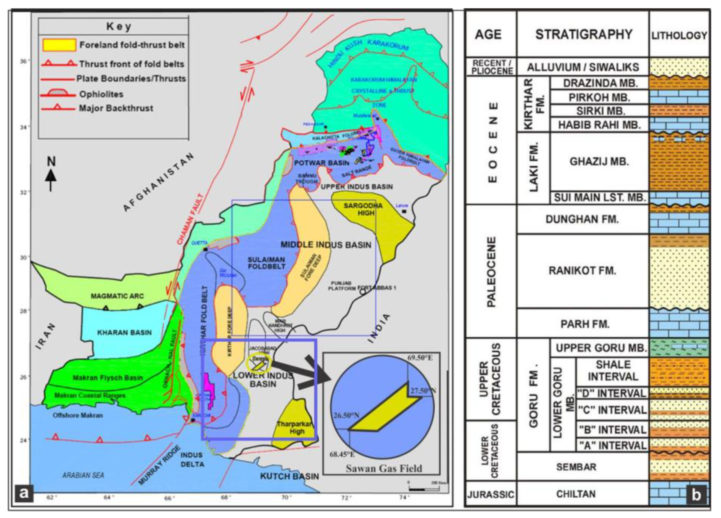
2. Geological Settings

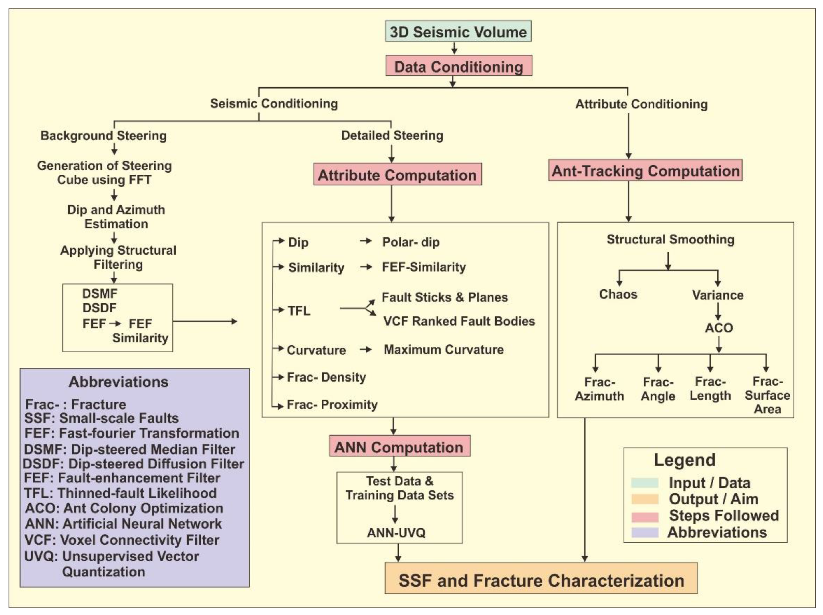
The study area (Sawan gas field) is located at the junction of the Middle Indus Basin and Southern (lower) Indus Basin of Pakistan. The lower Indus Basin is located in such a way that Indian Shield is located in the East; Sulaiman Fold, Thrust Belt, and Kirther Ranges are located in the West; Jacobabad-Khairpur High is located in the South; and Sargodha High is located in the North [59]. During the early Cretaceous time, the Indian plate drifted northward, where marine shales and limestones of the lower Cretaceous section of the Sembar and Goru formations were deposited on the northwest margin, whereas the carbonates were deposited on the northern shelf of the late Cretaceous [60]. The Precambrian basement of the basin and the majority of the Cretaceous rocks within the study area are tectonically stable and controlled [61,62,63,64]. Several structural lows and highs have been identified from the Precambrian, and these played important roles in the lateral and vertical thicknesses of the reservoir. Amongst these lows and highs, Jacobabad-Khairpur High, illustrated as a horst, is situated in our research area (Figure 1a). The Paleocene Ranikot clastics pinch out along the Khairpur High, which gives an indication of a preliminary Paleocene uplift episode that affects the Khairpur High. The enlargement of different sub-basins and complicated basinal topography during the Eocene suggests the occurrence of carbonate accumulations along with deep marls that were accumulated with Ghazij shales in the later stage. The tectonostratigraphic of the study area resulted from three tectonic episodes: erosion and uplifting in the late Cretaceous, basement rooted NNW–SSE wrench faults, and the recent uplifting of Jacobabad-Khairpur Highs of late Tertiary [65]. These faults were formed as a result of transtensional tectonics that were linked with Indian and Eurasian plate’s collision [66]. The stratigraphy of the study area incorporates Chiltan limestone (Jurassic age) at the base, which is overlain by different rocks of Sembar and lower Gou Formation (Cretaceous age) to alluvial rocks (Quaternary age). The primary lithologies of the lower Indus Basin are shelf carbonates and clastics, marine marls and shales, and turbidities [67] (Figure 1b). Several authors have researched the existence of wide Cretaceous deltaic settings and related shelf margins [68,69]

3. Methodology

The data were acquired from the Directorate General Concession Petroleum (DGPC), Ministry of Petroleum, Islamabad Pakistan. The seismic data were composed of a high-resolution 3D post-stack seismic volume that covered an area of approximately 25 km² of the Sawan gas field. The seismic grid contained an inline that ranged from 643 to 867, and the crossline ranged from 893 to 1031. A total of 225 inlines and 139 crosslines were used. The length of the inline was 3459.09, and the interval of the inlines was 25.03, whereas the length of the crossline was 5606.15, and the interval of the crosslines was 25.07. The sample value format was the International Business Machines (IBM) floating point. The sample interval was 4 ms, and the number of traces per sample was 1125.

The workflow employed for the current study incorporated the analysis of data conditioning, evaluation, and selection of seismic attributes, neural network computation, and artificial ant-tracking (Figure 2). In the first step, the data were conditioned, a process that incorporated seismic conditioning. The seismic conditioning included geostatistical and structural filtering to enhance and sharpen the structural features of the seismic data. In the second step, multiple structural attributes were analyzed to execute the selection process. The seismic attributes, which were extracting the best possible results of discontinuities, were shortlisted. In the third process, the shortlisted seismic attributes were tested and trained for the neural network analysis. In the fourth and last step of the study, the optimum attributes were selected and conditioned to process the ACO algorithm. The ACO was applied to evaluate the fracture network parameters.

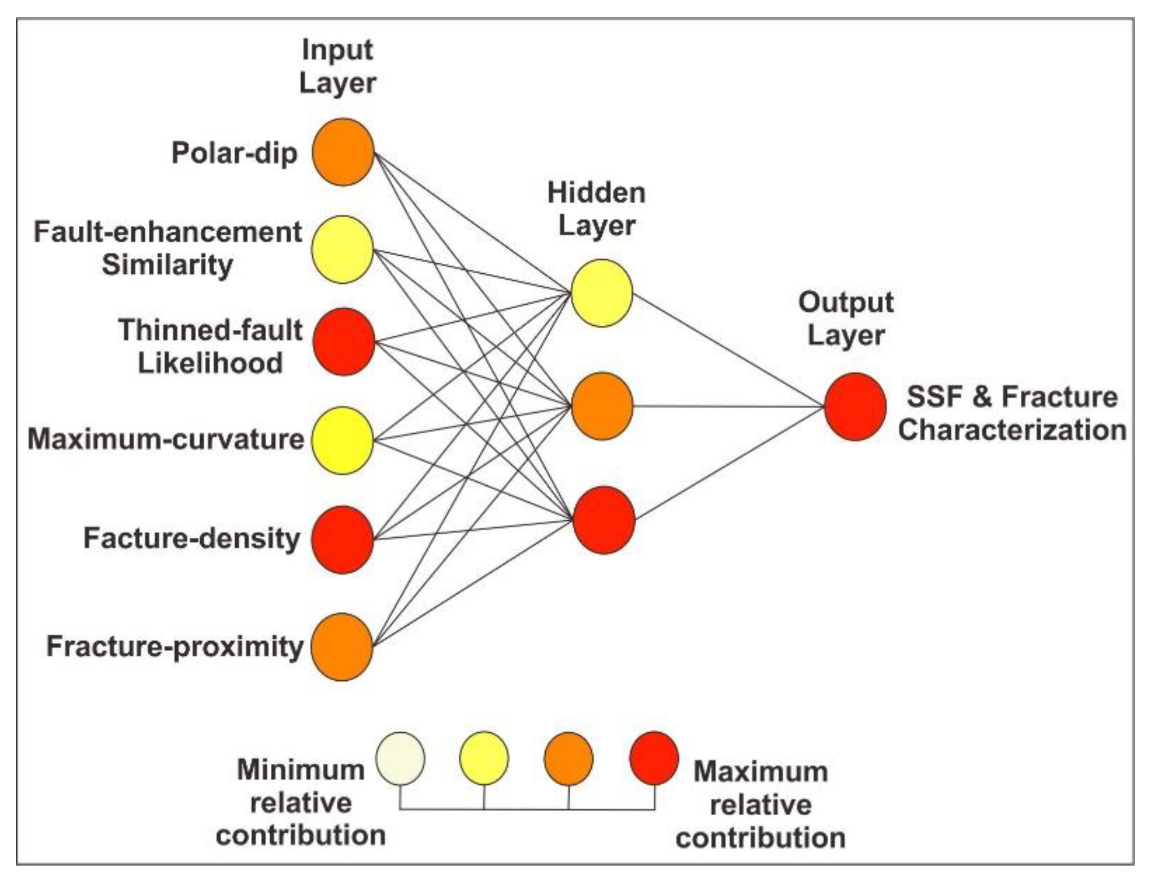
3.1. Artificial Neural Network

ANNs are computer-based mathematical models that are inspired by human brains that use continuous and parallel layers. These layers consist of nodes that are interconnected through weights [70]. These interconnected weights create associations amid the input layer and output layer of every node [50]. In the current study, unsupervised vector quantization (UVQ) was used for characterizing the faults and fractures. The UVQ used non-linear filtering and consisted of three steps: initialization, training, and application. The initialization evaluated the set of the classes, training improves these set of classes, and the application was used for the classification of the data. The number of classes was hard to determine in advance. Too many classes would have given redundant class centers, but too few classes would not have matched the seismic. Therefore, different quality checks were performed using different classes to proceed with the training.

In unsupervised training, network performance is tracked in a graph that shows the average match (confidence) of clustered input. Typically, the average match increases in a step-function. Each step indicates that the network has found a new cluster. Training can be stopped as soon as the average match has reached a stable situation (a straight line is obtained). Training that results in maximum match is accepted and is used to make the output maps.

Unsupervised classification maps are an advanced method that represents vectors that utilize a set of classes that lack user control [71]. The representing vector uses integrated, seismic attribute values that act as test data sets. Since the structural features are associated with erosional surfaces, reflection terminations, the variation of dip orientations, and changes in the amplitude signal, a set of seismic attributes are chosen as the input, which is very useful in identifying the network of discontinuities as an output.

3.2. Ant-Colony Optimization

ACO is a probabilistic method that is capable of resolving computational altercations that are constrained to finding paths in several ways [72]. It monitors the behavior of ants in the pursuit of food and fetching back to their nest by analyzing their paths [73]. The assemblage of the food is a unified effort of a group of ants for fetching the food, and they diffuse pheromones while making their way back; this diffusion appears as a fracture in a seismic volume. The diffusing pheromone can be recognized as an odor, and the scouting ants hunt the food by smelling this pheromone. The diffused pheromone is very volatile and, hence, evaporates. Thus, the solitary route remains, which is of shorter length and is followed by the majority of the ants to detect the noisy trends in the seismic data [11]. The scouting group of ants shows intelligence to extract the discontinuities that lead to colony optimization. The scouting ants detect their ideal track to food based on their intelligence and pheromone strategy [74], which is termed as swarm intelligence [75]. Swarm intelligence augments the discontinuous features in an edge-detection seismic volume since it tacitly tracks those trends that are continuous and are likely to be fault or fracture.

The algorithm supposes that the number of ants is proportional to the amount of diffused pheromone on a branch [15]. The pheromone on a branch at an intensity of path (i, j) at time t is denoted by ${\tau }_{ij}$, while the branch tracking $\rho$ (0 ≤ $\rho$ ≤ 1) and the pheromone amount per unit length of ant k at a path (i. j) is denoted by $\Delta {\tau }_{ij}{}^k$.

$${\tau }_{ij}\left(t+1\right)=\rho {\pi }_{ij}\left(t\right)+{\displaystyle \sum }\Delta {\tau }_{ij}{}^k. \left(t\right)$$

(1)

The branch length of ant k in a circle is represented by$Z_k$, and$\Delta {\tau }_{ij}{}^k=Q/Z_k$, where Q is a constant. The factor ${\mathsf{\eta }}_{ij}$ shows the visibility of the edge path (i, j), $\beta \left(\beta \ge 0\right)$ shows the relative importance of the path visibility, $\alpha \left(\alpha \ge 0\right)$ shows the relative importance of the branch, U represents the possible vertex set, and ${\rho }_{ij}{}^k\left(t\right)$ gives the transition probability of the ant k at time t. The probability of electing the branch was used in this study by using the 3D seismic volume to identify and sharpen the tracked faults and fractures [76].

$${\rho }_{ij}{}^k\left(t\right)=\{\begin{array}{c}\frac{{\left[{\tau }_{ij}\left(t\right)\right]}^{\alpha }{\left[{\mathsf{\eta }}_{ij}\right]}^{\beta }}{{{\displaystyle \sum }}_{l\in U}{\left[{\tau }_{il}\left(t\right)\right]}^{\alpha } {\left[{\mathsf{\eta }}_{il}\right]}^{\beta }}, j\in U\\ 0, otherwise\end{array}$$

(2)

The application of ant tracking entails several factors that extract fault information in a seismic amplitude volume. These factors incorporate an initial ant boundary, ant track deviation, ant step size, permissible illegal steps, obligatory legal steps, and stopping criteria [77]. The initial ant boundary governs that how narrowly the preliminary ant agents may be kept within a seismic volume. The ant track deviation illustrates the examining tolerance of the ants along the side of its tracking direction. A higher value of ant track deviation gives higher connections of the ant agents. The step size shows how far an ant can progress for every increment of its search. The permissible illegal steps showcase the ability of ants to image discontinuities further than the existing position. The obligatory legal steps factor works with the illegal step feature by acquiring the designated number of legal steps after an illegal step. The stop criteria also work with the illegal steps factor and do not permit the ants’ movement when plenty of illegal steps are involved.

3.3. Fault and Fracture Extraction

Interpreters usually manually mark the fault on the seismic section to carry out fault interpretations, which is a very difficult and time-consuming process to accurately interpret a fault. The uncertainty in manually interpreting faults and fractures is very high. The automatic extraction of faults and fractures can minimize human interference by providing the maximum proficiency and accuracy in extracting the faults [78]. Automated fault extraction technology allows interpreters to comprehend a fault and mark selections amid the extracted surfaces instead of generating surfaces. However, the outcome of the automatic fault extraction technology is constrained by various factors. These factors have a direct influence on the extraction of faults and fractures, and the factors are patch downsampling, minimum patch size, connectivity constraint, extraction background threshold, extraction sampling threshold, extraction sampling distance, and deviation from a plane.

Downsampling is effective in controlling the density of the various points of every patch. The minimum patch size sets the minimum number of points for fracture patches. The extraction background threshold and extraction sampling threshold control the least threshold signal value for the extraction and estimation of fracture patches. The extraction sampling distance controls the least distance by defining the radius amid extraction points. The deviation from a plane (DFAP) controls the orientation and deviation of a fracture from the surface of the plane. The DFAP plays an essential role in distinguishing fractures. A higher value of the DFAP decreases the possibility of extracting more fractures and vice versa. A DFAP of 9 was used in the study because the fractures merged into each other when a higher value of the DFAP was used.

3.4. Seismic Conditioning

It is necessary to apply various filters to obsolete the redundant noise while keeping geometrical features of seismic sections, because seismic attributes are susceptible to the noise within the seismic data [79]. For this purpose, multiple filters can be used to remove noise in seismic data; these filters are mean, median, and diffusion. The mean filter improves long-wavelength trends and reduces short-wavelength features. Moreover, it measures the mean amplitudes of provided data at chosen intervals to eradicate noise. The median filter measures the dip and azimuth of the targeted window and substitutes the dominant sample position with the median position of the amplitude. In addition, it also improves the spatial features, which are continuous, and reduces the noise of the seismic volume. Together, the duo of the mean and median filters reduces the noise while improving the signal-to-noise ratio that may deplete the fault and fracture features that can be solved using a diffusion filter [80]. The diffusion filter enhances the features that are continuous by keeping discontinuous features such as faults and fractures. If discontinuous features are detected, then smoothing does not take place, and filtering only applies to incoherent noise and insignificant stratigraphic features.

Initially, a geostatistical filter was applied here, and a steering cube was generated using the fast Fourier transformation (FFT) of the background steering. The steering cube was prepared by using the dip and azimuth values [48]. The background steering cube was comprised of the structural dip and contained multiple filters to study the dip-associated faults, fractures, and sedimentary structures. Hence, FFT was applied to delineate the stratigraphic and structural information in the seismic volume. The dip was computed within a cube of 3 × 3 × 3 samples around each sample of the seismic window.

The generated background steering cube was further incorporated while applying structural filtering. The dip-steered median filter (DSMF) was applied to remove random noise and to improve the dip and azimuth information of the generated steering cube. The noise removed was analyzed by the DSMF using the mathematics attribute. A diffusion filter was then applied on the dip-steered median filter to make the smoothing influence obsolete on the discontinuous features. The dip-steered diffusion filter (DSDF) enhanced the low-quality seismic data nearby faults and fractures. The two DSMF and DSDF filters were joined together to design an FEF. The FEF was based on a similarity threshold, and the data were smoothed (DSMF) away from the discontinuities and sharpened (DSDF) at the fault locations. Both similarity and steering cubes were incorporated in the study to establish a filter that had the same-sized window as the median filter. The results of the fault enhancement filter enhanced the sharpness of the faults and fractures, reduced the noise, and increased the smoothing of the reflectors. The FEF was then applied to the seismic volume to delineate the discontinuous features. The results provided a comparison of the original seismic (Figure 3a), dip-steered median filter (Figure 3b), dip-steered diffusion filter (Figure 3c), and the fault enhancement filter (Figure 3d) at inline 665. The results showed that the FEF effectively showcased the discontinuities marked by black arrows, which were not easily identified on the original seismic, DSMF, and DSDF data. The FEF and detailed steering cube were further used in the multi-attribute analysis to characterize the SSF and fracture network.

4. Shortlisting of Seismic Attributes

Multiple structural attributes were applied to delineate the maximum structural variations. Initially, the attributes were performed on the specific inlines or crosslines using various parameters. Those attributes that extracted the maximum information of structural discontinuities were selected. The shortlisted attributes were then applied to the whole seismic cube. A short overview and the results of the shortlisted geometric attributes are presented in this section.

4.1. Dip Attributes

Dip attributes were useful for evaluating the curvature and the dip-steered attributes, and they displayed the faults with displacement offsets, which were considerably less than the width of the seismic wavelet [11]. Dip attributes can be calculated using various components of the dip of a volumetric seismic cube. These include gradient structure tensor [81], discrete semblance-based dip searches [82], and wavenumbers and instantaneous frequencies [71].

Several dip attributes were applied using the detailed steering cube as the input that incorporated the azimuth, inline-dip, crossline-dip, and polar-dip to study the effect of dip on the structural features. The polar-dip was the true dip, which was measured from the horizontal, and its range was always positive. The dip in the direction of inlines was inline-dip, while the dip in the direction of the crossline was crossline-dip. The results of the dip attributes were analyzed on the time slices at 1780 ms, which delineated a fault that was present near the southwest of the study area shown by a red arrow and that was located around crossline 984 and inline 665 (Figure 4a–d). The results showed that the polar-dip proved to more beneficial in recognizing the discontinuities (marked by yellow arrows) compared to the crossline-dip, inline-dip, and azimuth results.

4.2. Curvature Attributes

Here, curvature measured the extent of the bending of a surface at a specific point using volumetric methods and analyzed the geometry distortion of the seismic volume instead of analyzing the variations in the seismic amplitude. Curvature is an effective tool to detect small scale faults and fractures with low displacement that would otherwise not be possible to identify with other fault attributes such as coherency. Compared to coherency, the curvature attribute draws the discontinuous features using minimum and maximum anomalies. Thus, it does not depict the precise position of a fault [83]. The surface of a reflector is supposed to be a quadratic surface to compute the curvature attribute [28].

$$z \left(x,y\right)=a{x}^2+b{y}^2+cxy+dx+ey+f$$

(3)

whereas,

$$a=\frac{1}{2} \frac{\partial p}{\partial x}$$

$$b=\frac{1}{2} \frac{\partial q}{\partial y}$$

$$c=\frac{1}{2} \left(\frac{\partial q}{\partial x}+\frac{\partial p}{\partial y}\right)$$

$$d=p$$

$$e=q$$

where p is the volumetric estimation of the inline-dip, q is the crossline-dip, and the coefficients become x = y = 0 [25].

Multiple curvature attributes were applied in the current study; these were maximum curvature, minimum curvature, the most positive and the most negative curvature attributes. Each of these curvature attributes had different parameters regardless of their signs to detect the fault and fracture discontinuities [11]. The results showed that the maximum curvature attribute was the most beneficial in terms of delineating the fractures in the study area (Figure 5a–d).

4.3. Similarity

Similarity attributes are a type of coherency that has a scale of 0–1 and that displays the similarity of the continuous features that are related to continuity of structural and stratigraphic trends [22]. Thus, similarity attributes are very effective in terms of delineating discontinuities. The algorithm of the similarity is semblance-based, which is evaluated for dips that have the maximum semblance selected for that dip [84].

$$\sigma \left(\tau ,p,q\right)=\frac{{[{\sum }_{j=1}^{J}u\left(\tau -p{x}_j-q{y}_j,x_j,y_j\right)]}^2+{[{\sum }_{j=1}^J{u}^H\left(\tau -p{x}_j-q{y}_j,x_j,y_j\right)]}^2}{J{\sum }_{j=1}^J\{{[u\left(\tau -p{x}_j-q{y}_j,x_j,y_j\right)]}^2+{[u^H\left(\tau -p{x}_j-q{y}_j,x_j,y_j\right)]}^2\}}$$

(4)

The triple ($\tau$, p, q) represents the local planar event at specific time.$\tau$, p, and q are the apparent dips at inline and crossline directions. H shows the Hilbert transformation of the real seismic trace (u).

A similarity algorithm was incorporated in the study to recognize the coherency in the inline and crossline directions, which allowed us to interpret the major discontinuities in specific directions. The full steered and non-steered similarity attributes were applied by using different windows to study the differences of the dip influence towards the discontinuities. Dip-steering eliminated the structural features of the similarity attribute, and precise results of faults were produced, whereas the non-steering similarity excluded the steering cube. The full-steering attribute proved to be more helpful than the non-steering attribute to delineate the discontinuous features (Figure 6a,b). Since the similarity attribute was very sensitive to the noise, the fault enhancement filter was also applied to the similarity attribute. The FEF improved the precision and sharpened the continuity of the faults. The discontinuities were compared through full-steered similarity, non-steered similarity, and FEF-similarity (Figure 6a–c). A comparatively large window was used for increased continuity, high-resolution results, and to extract the maximum information of the discontinuous features. Since the study area was relatively stable and the small scale faults and fractures are present. Thus, the effects of discontinuities were sharply analyzed through similarity attributes. The results of FEF-similarity were more continuous and sharp than the dip-steering similarity attributes. The results were also analyzed on the FEF similarity cube, which showed the significant discontinuities (yellow arrows) in the studied seismic volume (Figure 6d).

The FEF-similarity highlighted the major and thick discontinuities in the study cube. Still, these low similarity values were not able to detect the minor discontinuities and the association between these major and minor discontinuities. To study the connectivity of the discontinuities, TFL was applied.

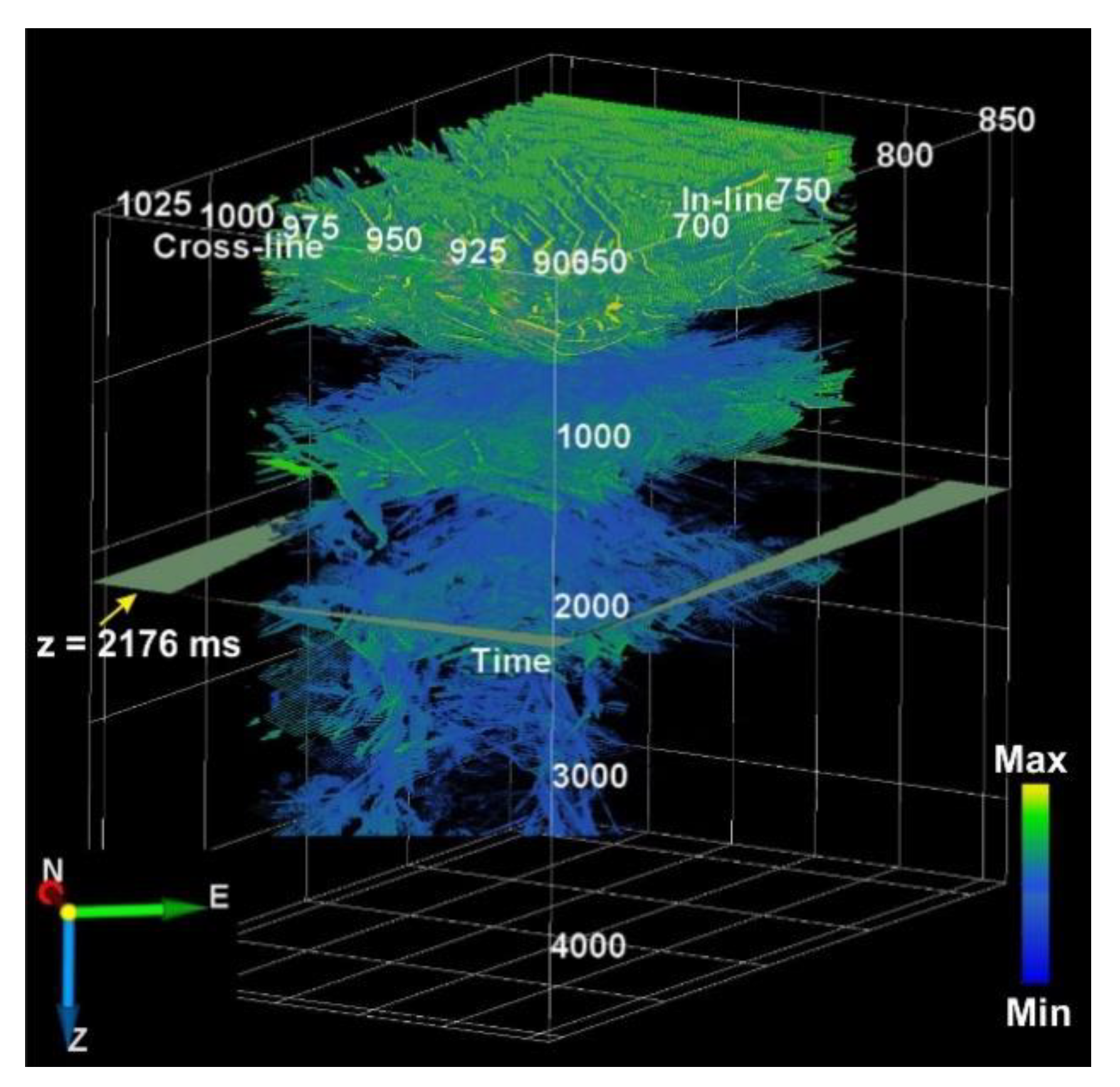
4.4. Thinned Fault Likelihood

TFL is a novel innovative fault attribute that yields precise and exact discontinuities. It is defined as a power of semblance, and it has a range between 0 and 1. It generates seismic volumes with razor-sharp edges that are very well suited for structural interpretation. The algorithm detects the range of fault dips to find the maximum likelihood to delineate the fractures in the area of interest and gives razor-sharp fault images on vertical sections and horizontal slices. A comprehensive study by [35] proposed a method of fault likelihood to recognize locally planar discontinuity. The TFL technique measures the likely combinations of dips and strikes to obtain a solitary direction, which gives the maximum fault likelihood for every sample image [35].

The TFL for every sample was documented in TFL images across the whole seismic cube, as shown in Figure 7. The inserted slice on the resultant TFL cube at 2176 ms showed that the area was affected by small scale fractures. The results showed that maximum fractures were present at the top from 600 to 900 ms, which were large scale fractures of higher lengths. Additionally, the TFL values were at minimum below 3000 ms, which showed the presence of relatively fewer fractures of a very small scale.

The discontinuity features were further observed using the fault discontinuity attribute volume to create and rank the fracture bodies. The resultant TFL volume was used as input for estimating the fracture bodies using the VCF. The VCF is an effective tool to create continuous bodies based on the amplitudes in a stored volume. A voxel is defined as the volume around one sample. The sample’s interconnection was computed based on amplitude criteria and geometrical spreading settings. The voxel connectivity filter was applied using the envelope of the amplitudes, which were higher than the 0.6 value; the envelope was defined for the fracture bodies to be computed. The propagation was done in all directions (26) using the six faces, twelve edges, and eight corners adjacent to the current seed. The bodies that were larger than 100 voxels were processed as relatively large scale fractures, and the output volume was processed using the body-size. The results of the generated connected fracture bodies were displayed using the voxel connectivity filter, as shown in Figure 8a. The results showed the orientations of the connected small scale and large scale fracture bodies. The facture bodies were oriented mostly in the east–west directions, and large-scale fracture bodies were present at the top, whereas the small scale fracture bodies were present at the bottom of the study area.

The fracture planes and sticks were also extracted using the discontinuous TFL volume as input. The fracture planes proved to be quite beneficial in recognizing the sweet spots for prospect evaluation, field development, and future drilling of exploration and appraisal wells [85]. The fractures were interpreted and visualized on the cube as a stick, and all sticks that belonged to one fracture were merged into a single stick set. Thus, a single fracture stick set was comprised of an unordered collection of the interpreted sticks. The minimum TFL value of 0.01 was used in the current study. The minimum value of sticks per fracture was applied, which helped to identify the small scale fractures that had small throws. The minimum vertical overlap rate of 0.6 was used to extract maximum tilted fractures, because a value greater than 0.6 may have extracted maximum fractures with a risk of picking up more noise. The minimum fracture length per z-slice of 250 was applied to extract the maximum fractures with smaller heaves. The feature of merging fractures along z-slices was also applied, and this increased the possibility of capturing the lateral continuity of fractures. The results of the extracted fracture planes and sticks generated for the seismic study volume are shown in Figure 8b.

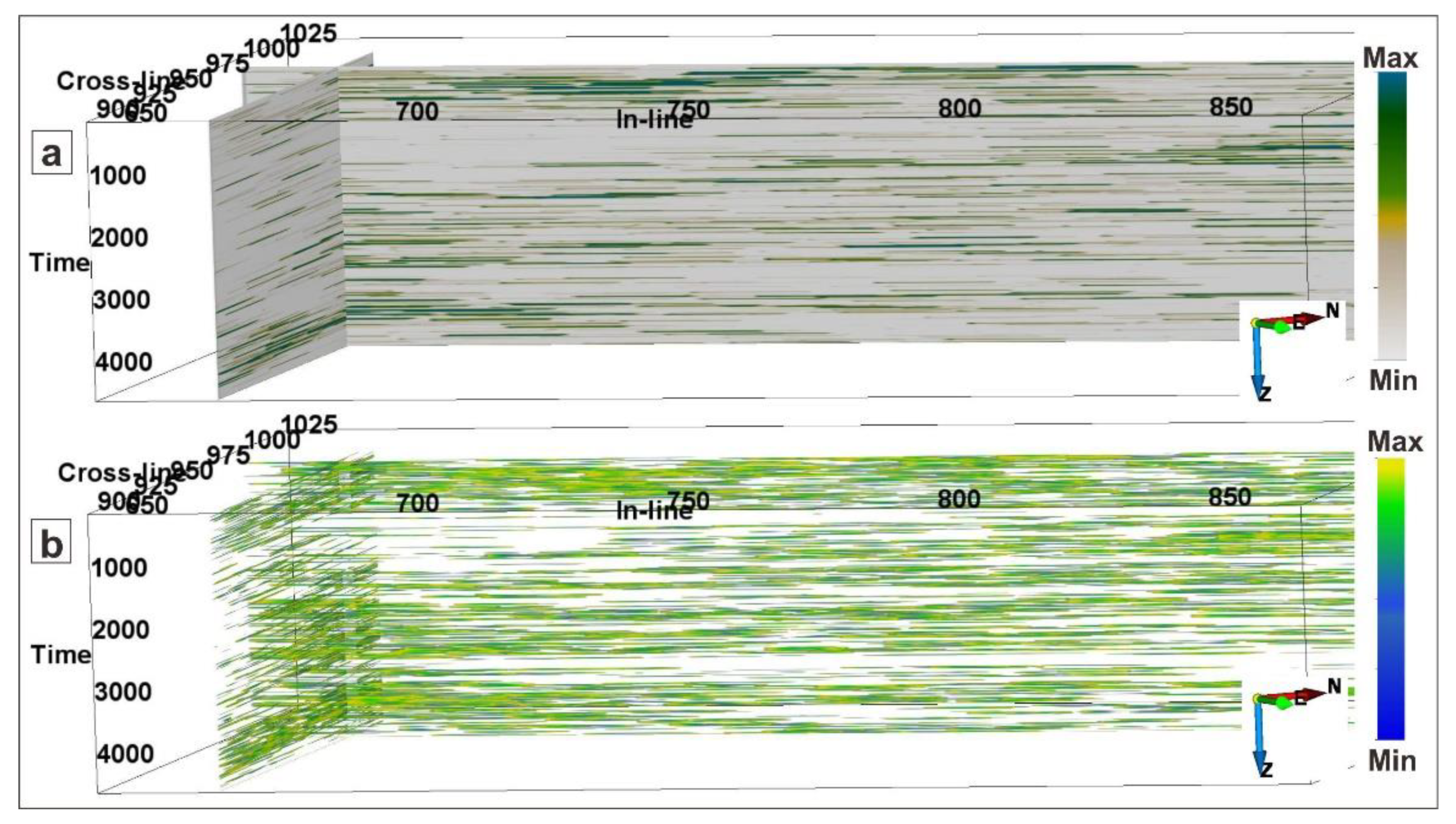
4.5. Fracture Density

Fracture density highlights regions of high-density fractures. It requires a radius for scanning and computing the density of fracture anomalies. Thus, it is defined as the ratio of the number of traces classified as fractures to the total number of traces present in a circle of given radius along z-slices. Here, the fracture density showed the improved visualization of potential fracture anomalies. The maximum curvature attribute was used as an input for the generation of fracture density. The results of the fracture density are shown in Figure 9a. The results of the fracture density showed maximum values along the erosional surfaces and in the proximity of the fracture activities. It was also essential to consider that structural discontinuities, such as fractures, did not represent the flow channels because channels and fractures had different morphology. Moreover, the regions of maximum fractures were more conductive than regions of minimum fracture activities.

4.6. Fracture Proximity

Fracture proximity helps to identify the locations of maximum fracture activity in a specified radius. It computes the lateral distance (i.e., along z-slice) from a trace location classified as a fracture. Fracture proximity is also helpful in tracking radius for drilling purposes. The maximum curvature attribute volume cube was used as an input here for the generation of fracture proximity. The fracture proximity highlighted the distance from the fracture center. The result of the fracture proximity is shown in Figure 9b and suggested that the studied seismic volume was mostly affected by fracture activities because there were multiple regions across the whole studied area that showed the distance from the fractures.

These fracture regions were also displayed as generated 3D volume that showed high-density and maximum fracture activity regions (marked by yellow arrows) (Figure 10a,b).

5. Neural Network Computation

After the selection process of seismic attributes, both supervised and unsupervised neural networks can be used to evaluate discontinuities [11]. In the current study, UVQ was used because the TFL and fracture density identified the most likely fault and fracture features. Therefore, the ANN was computed using the unsupervised algorithm.

The fracture positions were connected with bed terminations that were categorized by maximum variation of dip values, maximum curvature attributes, low values of similarity, maximum values of TFL, and maximum values of fracture density and fracture proximity. Henceforth, those seismic attributes that were already shortlisted in the current study (such as polar-dip, FEF-similarity, TFL, maximum-curvature, fracture density, and fracture proximity) were chosen for neural network computation.

The shortlisted seismic attributes were tested for input, and, after various quality checks (QC’s), they went through a training program for ANN computation by using the UVQ of ten classes to yield an optimal output. The neural network tried to cluster the set of vectors, and similar vectors went into the same segment. Segmentation was performed using the shortlisted multi-attributes, and class centers were analyzed. The ANN–UVQ process comprised three distinct layers: the input, hidden layer, and output layers. These layers were connected with one another to make an entirely connected UVQ network that was comprised of ten nodes. Among them, the input layer consisted of six nodes (three related to the hidden layer), and the output layer was represented by one node. (Figure 11). The number of vectors assigned to each node and their average match to the corresponding class center were also analyzed, appearing as a robust classification.

The input test data and the training data were applied in training, and this was continued until a straight line was obtained (that resulted above 75%), which suggested minimum error. The training was then ceased, and the results of the network were analyzed regarding the volume, section and time slices. The relative contribution of the seismic attributes UVQ classification is shown in

Table 1. Sensitivity table illustrating the input node relative weights of every attribute used for the ANN–UVQ.

Attributes	Relative Contribution
Polar-dip	34.2
Fault-enhancement Similarity	31.9
Thinned-fault likelihood	95.4
Maximum-curvature	50.3
Fracture-density	100.0
Fracture-proximity	70.2

.

The results of the ANN–UVQ highlighted the fracture network using the weighted average of all the selected attributes. The seismic cube and the seismic section of the ANN–UVQ showed the discontinuities with maximum probability, as shown by the red rectangles in Figure 12a,b. The maximum likelihood of fractures was also computed at different slices, which indicated that maximum fractures were present at slice 700 ms. In contrast, the probability of fractures at 2180 ms was minimum (Figure 13a–d). Since the reservoir in the study area lies from 2100 to 2400 ms. The likelihood of the fractures was also analyzed at 2250, 2300, 2350, and 2400 ms, thus giving the idea of the trend of the fractures in the study area (Figure 13e,f). These slices could be further exploited for future drilling prospects, if further evaluated.

6. Ant-Tracking Computation

6.1. Attribute Conditioning

Before applying the ant-tracking algorithm to the attributes, the conditioning of multiple attributes was done to calibrate the suitability of finding the best outcomes for fault and fracture delineation. Therefore, attribute conditioning was used to improve the signal-to-noise ratio to show continuous fault and fracture features.

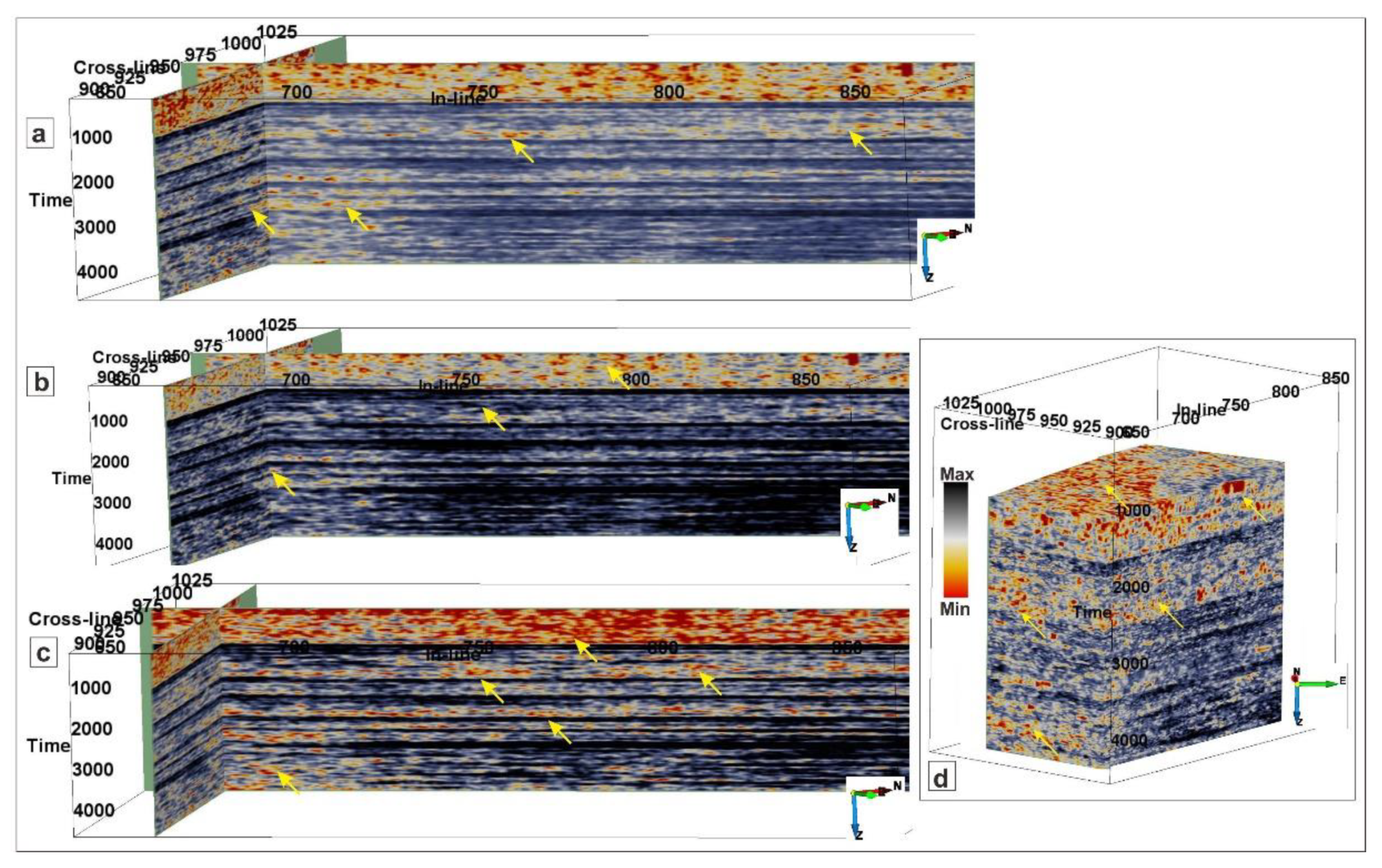
6.1.1. Structural Smoothing

The obtained amplitude volume of the Sawan gas field interrupted amplitude continuity at several locations. Henceforward, structural smoothing based on the Gaussian smoothing algorithm (GSA) was incorporated to reconstruct the discontinuities. The structural smoothing measured the guided signal of the structural features by enhancing the continuity of the reflectors [69]. The azimuth and dip parameters were used to measure the structural features. The Gaussian smoothing algorithm was then used adjacent to these structures. GSA is an efficient tool to use before auto-tracking to steady results [77]. The estimation of structural smoothing use the value of the Gaussian filter, which governs the number of traces horizontally and samples vertically. The value symbolizes the standard deviation of the applied Gaussian filter. The maximum value was used in the study so that the maximum number of traces and samples could be smoothened. A standard deviation of 1.5 was applied to get the smoothed volume.

6.1.2. Chaos

The term chaoticness is used for highlighting the reflector discontinuities using differences in azimuth and dip [77]. The maximum value of chaoticness indicates the regions of discontinuities such as fractures, faults, or unconformities [86]. The signal pattern of the chaotic texture also indicates the migration of gas pathways. Here, the 3D map of the chaos attribute showed many discontinuities in the upper portion of the seismic section, while there were fewer discontinuities in the lower area. (Figure 14a).

6.1.3. Variance

Variance is an edge detection technique, and it calibrates the dissimilarities from a mean value to produce computationally proficient results that are much sharper than coherency [86]. The variance was incorporated to reduce the noise and to yield possible vertical smoothing. The variance was applied using the dip to highlight discontinuities. The value of the 0.6 plane confidence threshold was used for evaluating the discontinuities.

The variance attribute was able to more precisely and sharply detect discontinuities than the chaos attribute (Figure 14b). Henceforth, the variance was further used in the ant-tracking analysis for fault and fracture study.

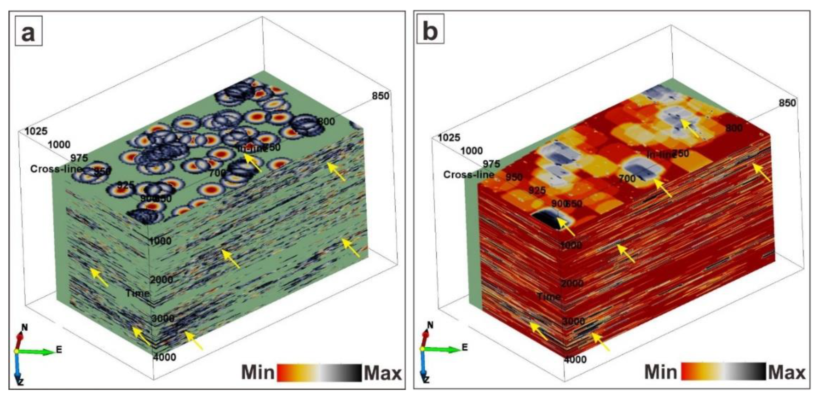
6.2. Ant-Tracking Result

Ant-tracking was used to extract the faults from the pre-processed variance volume. Initially, structural smoothing was applied to enhance the continuity of the structural features (faults and fractures) using the Gaussian smoothing algorithm, and then the variance attribute was used as an input on the structural smoothing attribute to get the ant-tracking attribute; the results were displayed at various locations of inline 665 and crossline 972. The results showed that the original seismic volume interrupted amplitude continuity (Figure 15a,e), which was rectified with the structural smoothing effect to enhance and sharpen the visibility of discontinuous features (Figure 15b,f). The variance attribute was applied to the structural smoothing seismic volume, which showed the discontinuous features (Figure 15c,g). The results of the ant-tracking applied to the variance attribute precisely characterized the faults and fractures (Figure 15d,h).

The direction of fractures was evaluated by applying various azimuthal filters to the ant-tracking algorithm. The aim was to restrict the ants in specific directions to get optimum results. The ant-tracking using east–west (E–W) and north–south (N–S) azimuthal filters were applied to recognize the orientation of the fractures. The results showed that the north–south azimuthal filter helped to identify the north–south oriented fractures. In contrast, the east–west azimuthal filter was beneficial in recognizing the east–west directed fractures. Moreover, the results of applied filters revealed that the study area has more east–west oriented fractures than north–south oriented fractures (Figure 16a–c).

6.3. Automatic Fault and Fracture Extraction Using ACO

Fracture detective attributes generate responses along the surfaces of a fracture and help to detect automatic fracture interpretations. These attributes may incorporate noises and residual responses, which makes it very challenging to interpret fractures. To overcome these challenges to map the fractures, attributes conditioning was applied through an innovative approach of the ACO algorithm.

The 2D (bird’s-eye view) (Figure 17a) and the 3D view (Figure 17b) of the extracted fractures show the orientation of fractures. Fracture surfaces generated in the ACO method are commonly fractured segments instead of fracture surfaces [87].

The results of the extracted fracture network were displayed on the stereonet, which showed that 607 visible patches (fractures) were present, and these were scattered in different orientations. The results of the dip azimuth showed that most fractures were clustered in the NW–SE direction (Figure 18a). The histogram of the fracture dip angle showed that the most fracture patches lie between 16° and 32° (Figure 18b). The histogram of the fracture length suggested that most fractures have fracture lengths between 200 and 500 m (Figure 18c). The histogram of the fracture surface area indicated that many fracture patches are present between surface areas of about 10,000–30,000 m² (Figure 18d).

All the results of the histograms showed that the frequency of the number of patches decreased with increasing fracture angle, fracture length, and fracture surface area. The results showcased the presence of small-to-medium scale fracture segments with an average length of about 625 m and that were gently dipping to about average 38°. The corollary is that the overall results of the workflow showed that these numerous fractures played an important role in the development of the reservoir potential in the Sawan gas field.

The current study also revealed a fault in the study area that had been previously overlooked. The fault is a small scale fault, and the orientation of the fault is NNW–SSE (Figure 19a–c). The throw and heave of the fault are minor and are present in the Upper Goru Formation of Upper Cretaceous age. This NNW–SSE oriented fault distributes the study area into east and west parts and is named the Sawan fault [65].

The generated steering cube for the dip and azimuth estimation, as well as the application of structural filtering to remove the noise, considerably enhanced the sharpness and continuity of the structural features such as SSFs and fractures. Hence, the current study provided a workflow that put forward an effective data conditioning method for fault and fracture identification. Moreover, the adopted workflow also presented an advanced and novel approach of attribute computation using ANN–UVQ for the identification of the fracture network.

The current study proved helpful in identifying the fault and fracture probabilities of the study area. However, various technical aspects can be upgraded for future works. Instead of using the unsupervised ANN, other unconventional techniques, like the supervised ANN such as multi-layer perceptron network (MLP), can be used. The limitation of the presented work is that our ANN model was intended and trained to trace the fault and fracture probabilities only. In future research, the ANN model should be designed in such a way to extract information regarding fault slip and fault displacement. Another limitation of our work is that the current research lacked the usage of image log and core data, which were unfortunately not available. For future study, the use of image logs, conventional logs, and their correlation with core data along with 3D seismic is suggested to give a more comprehensive picture of large and small scale fracture development in the study area.

7. Conclusions

The current study provided an effective and advanced workflow for the identification of SSFs and fractures of a heterogeneous sand reservoir. The conclusions are as follows;

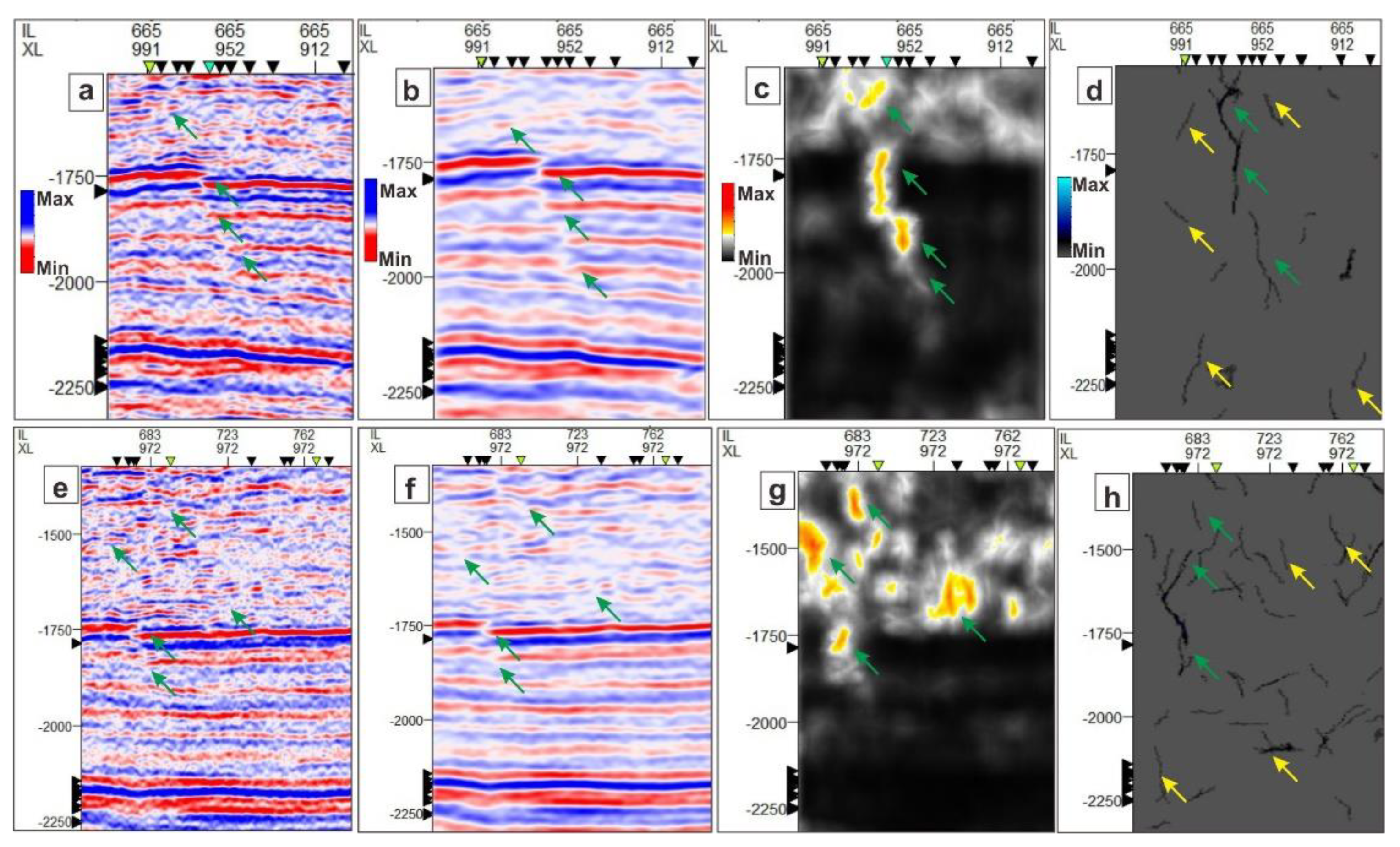
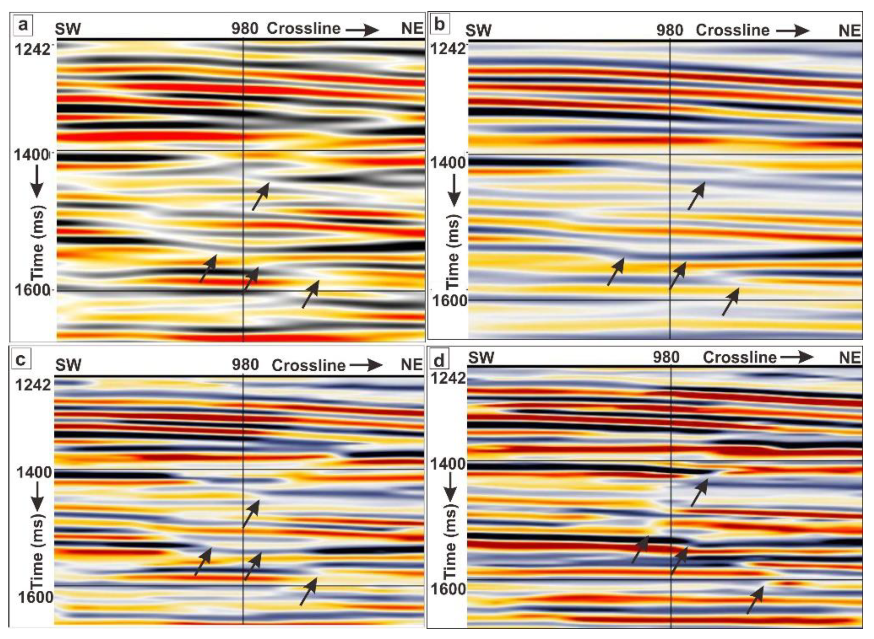
• The structural features of the seismic volume were enhanced and sharpened using a DSMF, a DSDF, and a FEF. The FEF proved to be most effective in recognizing discontinuities.
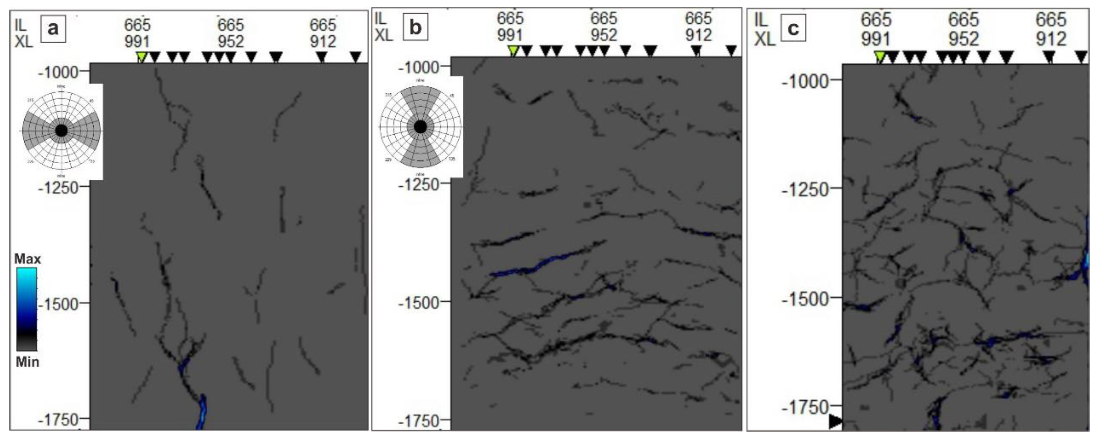
• The novel technique of TFL was used for the generation of the likelihood, dip and the strike of the seismic cube. The generated TFL cube highlighted the maximum likelihood of the dips and the strikes of the fractures. The interconnected VCF ranked fracture bodies, automated fracture surfaces, and fracture sticks using TFL, and it delineated the orientations of fractures.
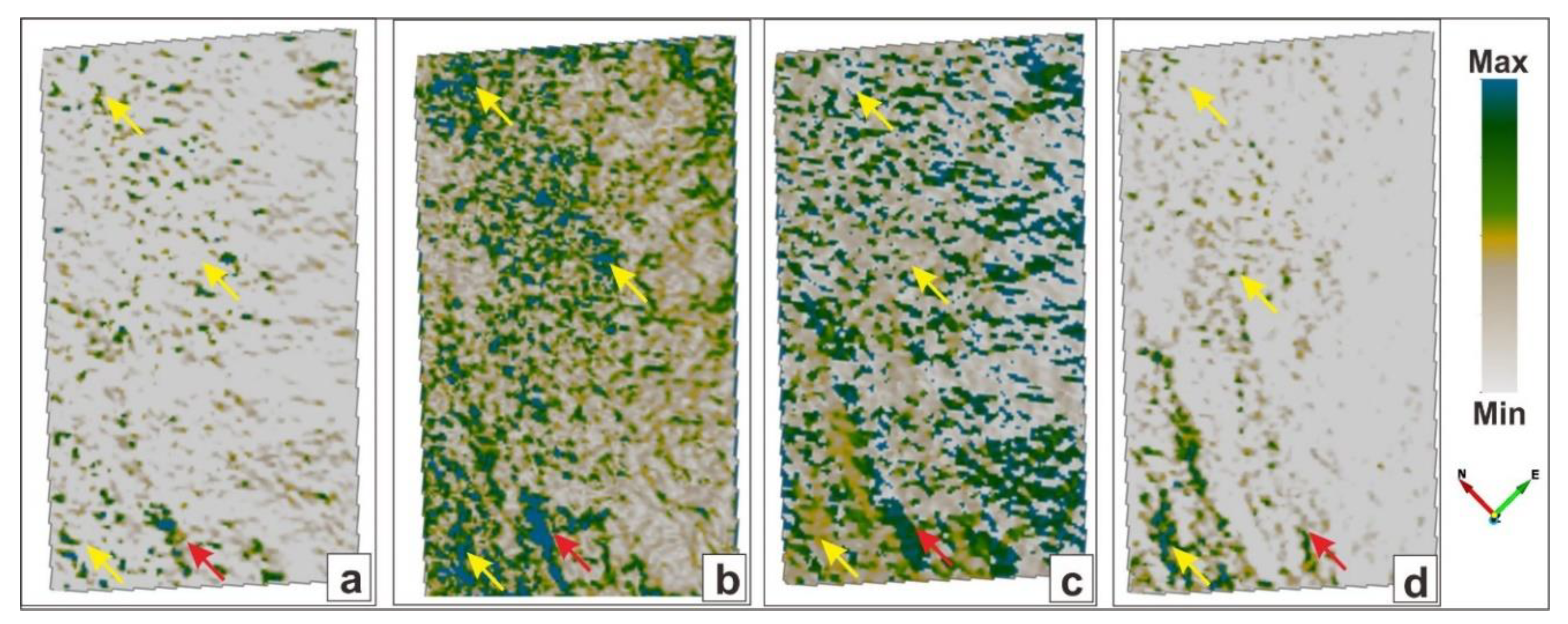
• The use of fracture density and fracture proximity are powerful tools in visualizing the high-density and maximum fracture activities regions that can be exploited for future drilling.
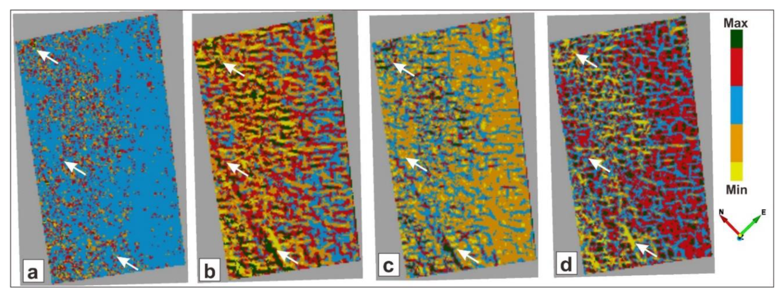
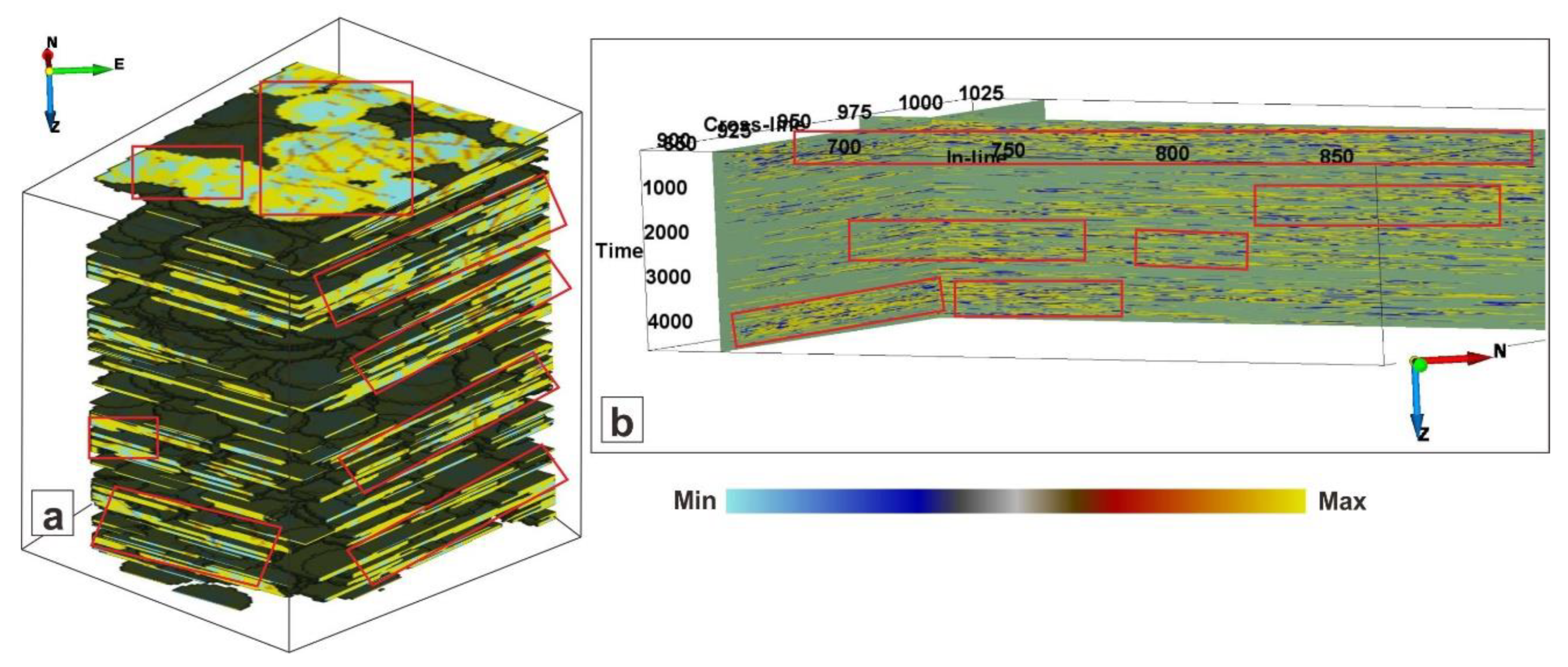
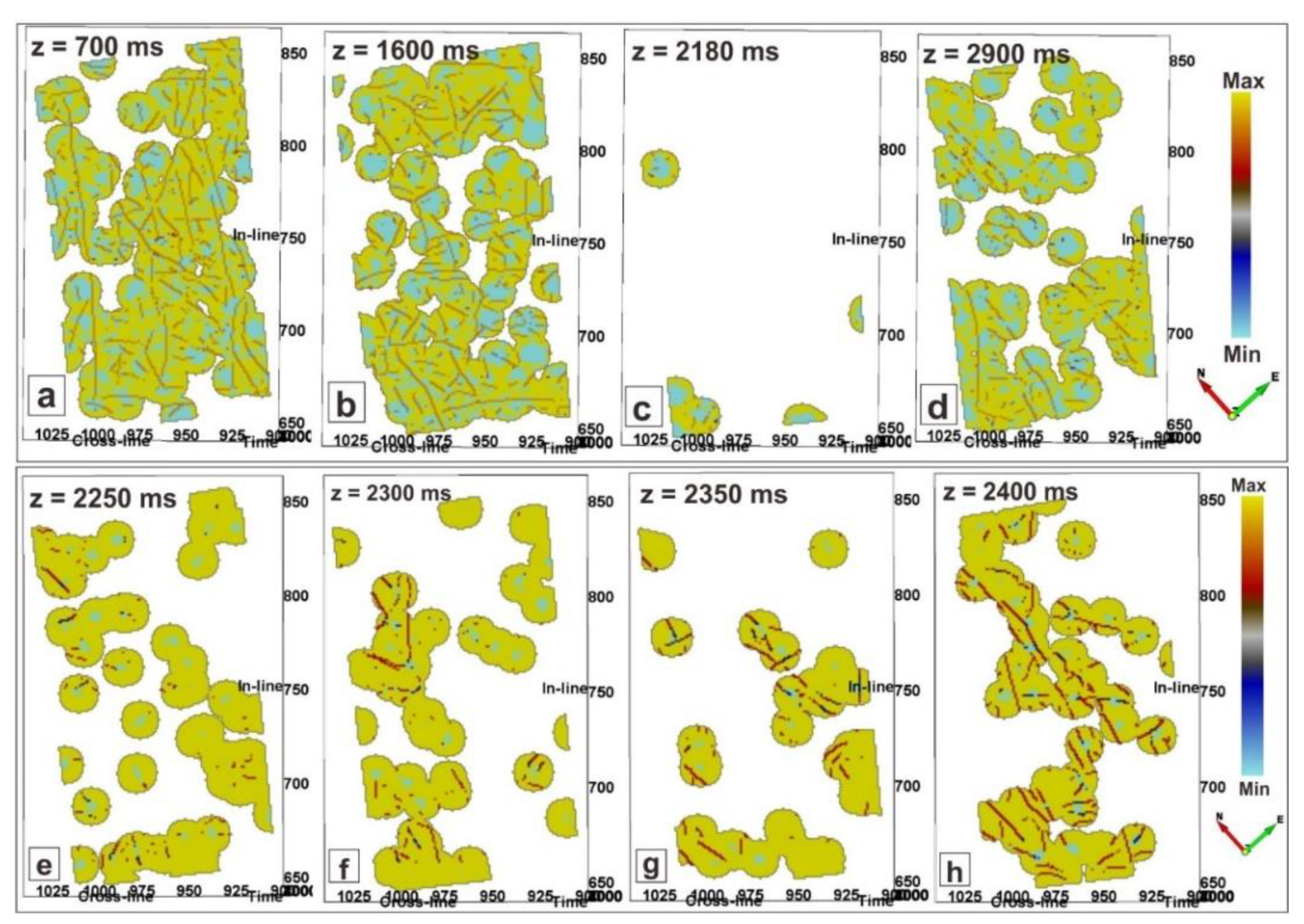
• The ANN–UVQ using multi-attribute computation identified the maximum and subtle fault, as well as the fractured locations and orientations, which will be beneficial for the field development of the study area.
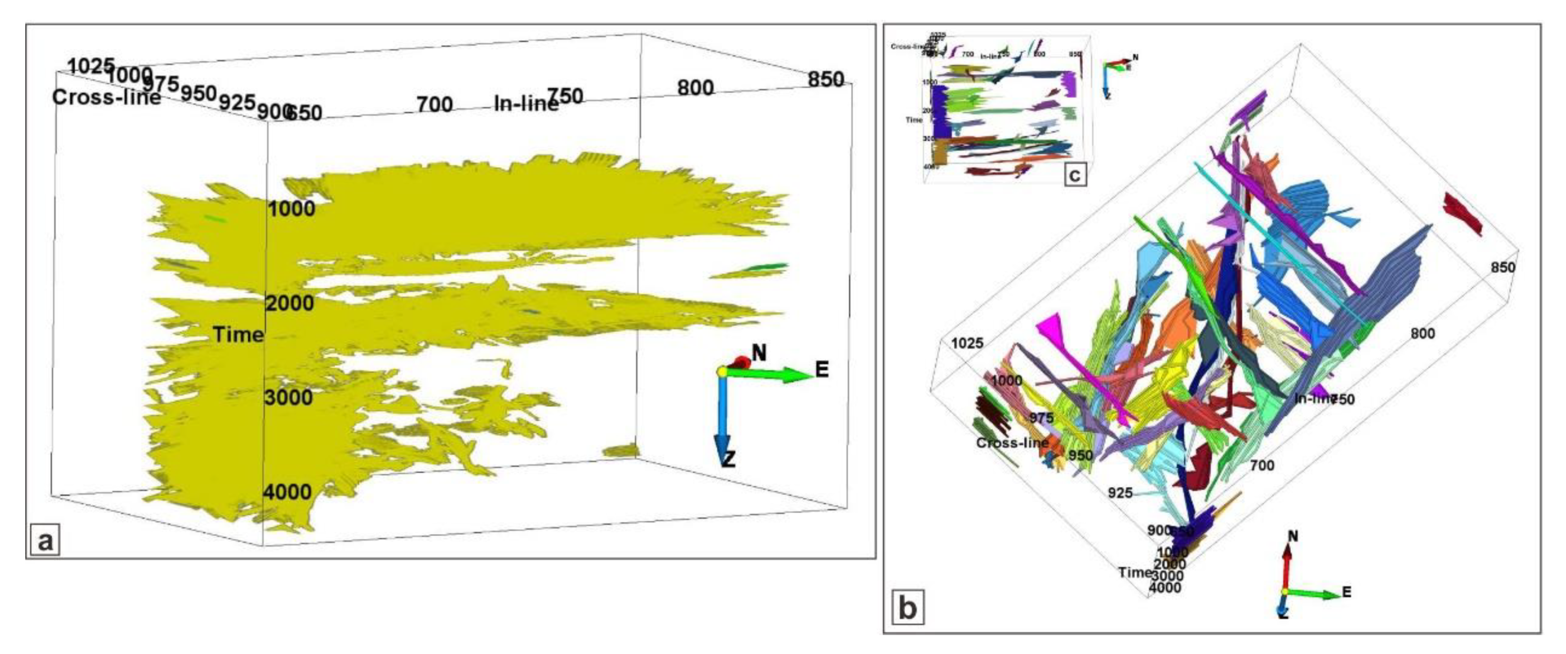
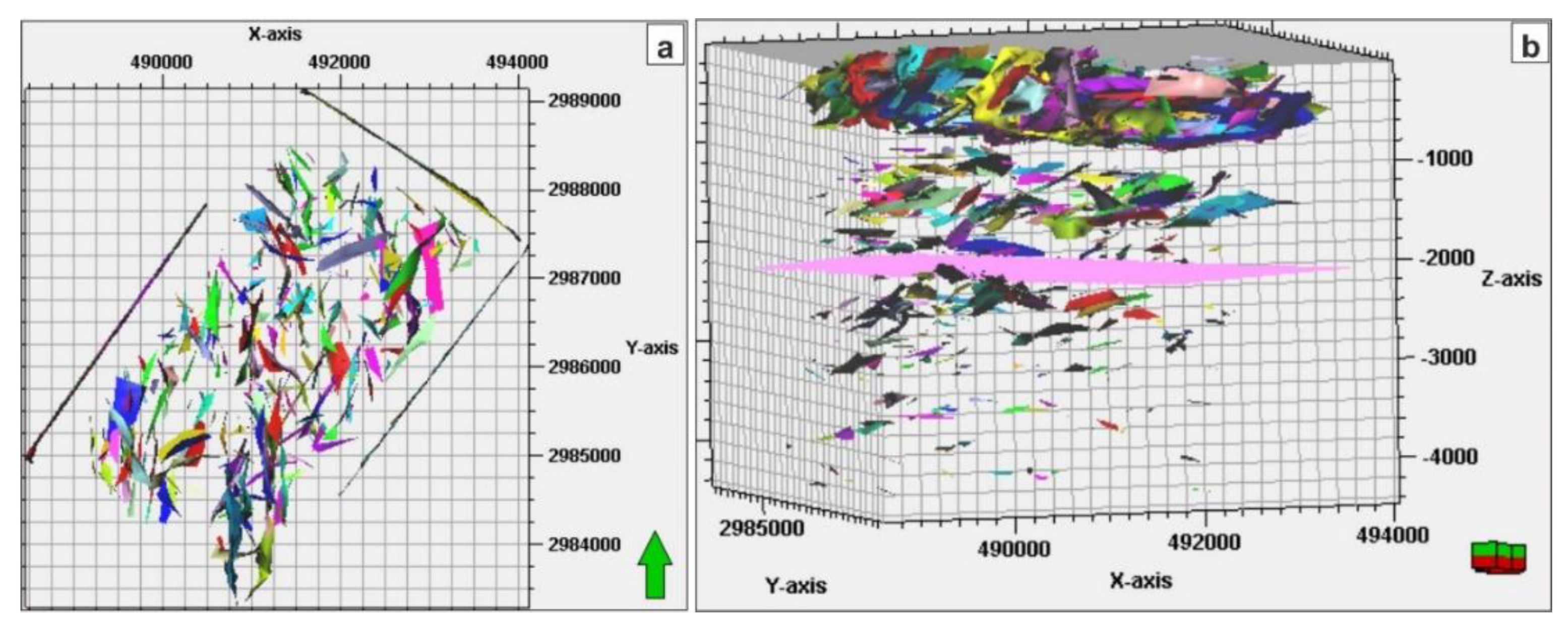
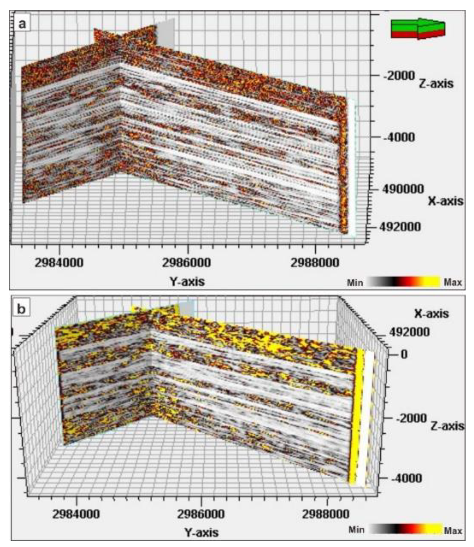
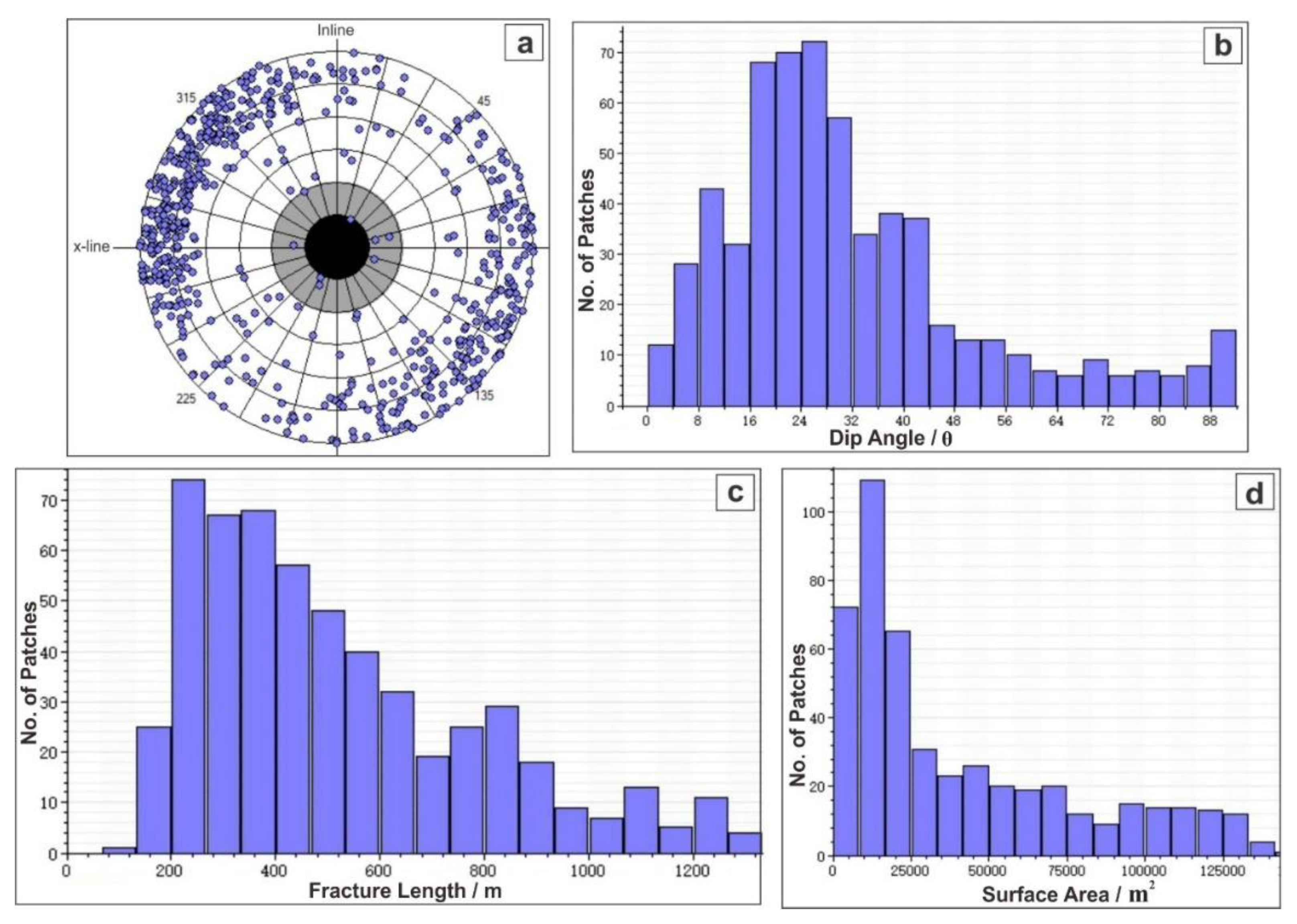
• The ACO algorithm was effectively applied to study the dip, length, azimuth, and surface area of the fractures. The results of the ACO showed that there are more E–W oriented fractures than N–S fractures. The automatic extraction of fractures using ACO identified 607 subtle fracture patches. The dip azimuth of these fractures are clustered at SE–NW direction, the dip of most of the fractures lies between 16° to 32°, the fracture length lies between 200 and 500 m, and the surface area lies between 10,000 and 30,000 m².
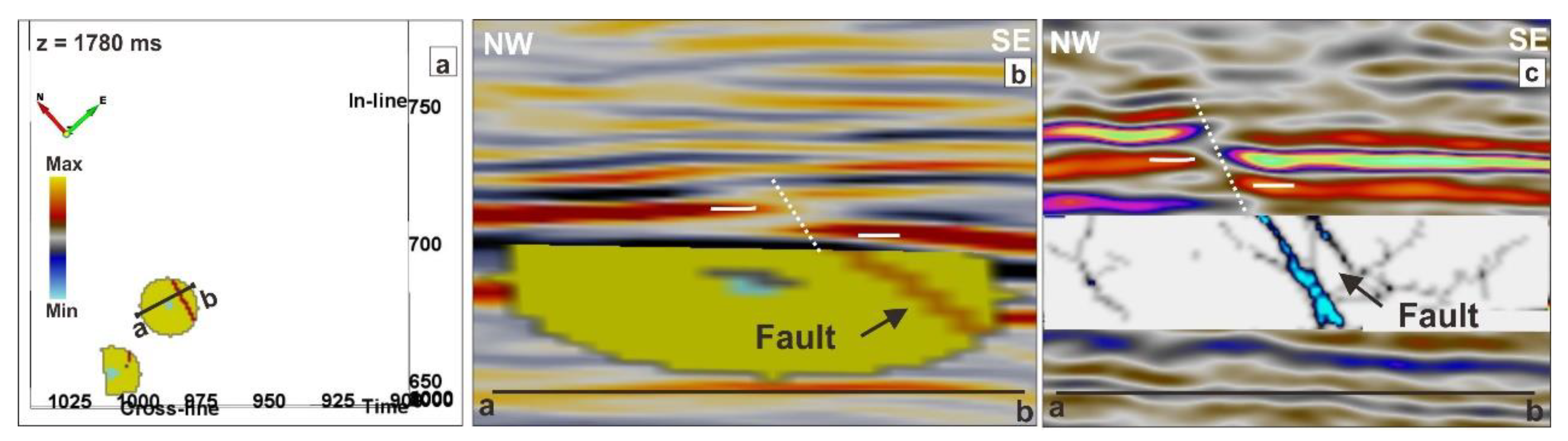
• The ANN–UVQ and ACO revealed an NNW–SSE oriented fault that has minor heave and throw.
• The adopted workflow in the study for the recognition of SSFs and fractures is automated, adaptive, time-saving, cost-saving, effective, innovative, and novel. The applied workflow is advanced and can be further utilized for the delineation of SSFs, large-scale faults, and fractures in any reservoir worldwide.

References

1. Clausen, O.R.; Korstgåd, J.A. Small-scale faulting as an indicator of deformation mechanism in the Tertiary sediments of the northern Danish Central Trough. J. Struct. Geol. 1993, 15, 1343–1357. [Google Scholar] [CrossRef]
2. Jia, C. Characteristics of Chinese Petroleum Geology: Geological Features and Exploration Cases of Stratigraphic, Foreland and Deep Formation Traps; Springer Science & Business Media: Beijing, China, 2013. [Google Scholar]
3. Yin, S.; Lv, D.; Ding, W. New method for assessing microfracture stress sensitivity in tight sandstone reservoirs based on acoustic experiments. Int. J. Geomech. 2018, 18, 04018008. [Google Scholar] [CrossRef]
4. Boro, H.; Rosero, E.; Bertotti, G. Fracture-network analysis of the Latemar Platform (northern Italy): Integrating outcrop studies to constrain the hydraulic properties of fractures in reservoir models. Pet. Geosci. 2014, 20, 79–92. [Google Scholar] [CrossRef]
5. Wennberg, O.P.; Casini, G.; Jonoud, S.; Peacock, D.C. The characteristics of open fractures in carbonate reservoirs and their impact on fluid flow: A discussion. Pet. Geosci. 2016, 22, 91–104. [Google Scholar] [CrossRef]
6. Zeng, L. Microfracturing in the Upper Triassic Sichuan Basin tight-gas sandstones: Tectonic, overpressure, and diagenetic origins. AAPG Bull. 2010, 94, 1811–1825. [Google Scholar] [CrossRef]
7. Zhou, Y.; Ji, Y.; Zhang, S.; Wan, L. Controls on reservoir quality of Lower Cretaceous tight sandstones in the Laiyang Sag, Jiaolai Basin, Eastern China: Integrated sedimentologic, diagenetic and microfracturing data. Mar. Pet. Geol. 2016, 76, 26–50. [Google Scholar] [CrossRef]
8. Zhang, M.-L.; Bao, Y.; Zhang, S.-Q.; Liu, G.-Z. A Recognition Technology of Low Order Faults and Relative Application. Sci. Technol. Eng. 2011, 11, 7790–7901. [Google Scholar]
9. Ameen, M.S.; Hailwood, E.A. A new technology for the characterization of microfractured reservoirs (test case: Unayzah reservoir, Wudayhi field, Saudi Arabia). AAPG Bull. 2008, 92, 31–52. [Google Scholar] [CrossRef]
10. Peace, A.; McCaffrey, K.; Imber, J.; van Hunen, J.; Hobbs, R.; Wilson, R. The role of pre-existing structures during rifting, continental breakup and transform system development, offshore West Greenland. Basin Res. 2018, 30, 373–394. [Google Scholar] [CrossRef] [Green Version]
11. Basir, H.M.; Javaherian, A.; Yaraki, M.T. Multi-attribute ant-tracking and neural network for fault detection: A case study of an Iranian oilfield. J. Geophys. Eng. 2013, 10, 015009. [Google Scholar] [CrossRef]
12. Baytok, S.; Pranter, M.J. Fault and fracture distribution within a tight-gas sandstone reservoir: Mesaverde Group, Mamm Creek Field, Piceance Basin, Colorado, USA. Pet. Geosci. 2013, 19, 203–222. [Google Scholar] [CrossRef]
13. Riaz, M.S.; Bin, S.; Naeem, S.; Kai, W.; Xie, Z.; Gilani, S.M.M.; Ashraf, U. Over 100 years of faults interaction, stress accumulation, and creeping implications, on Chaman Fault System, Pakistan. Int. J. Earth Sci. 2019, 108, 1351–1359. [Google Scholar] [CrossRef]
14. Chenghao, L.; Liquan, G.; Wei, Z.; Fa, Y. Fine interpretation of mine geological structure through ant tracking technology. Coal Geol. China 2013, 25, 55–59. [Google Scholar]
15. Hu, J.L.; Kang, Z.H.; Yuan, L.L. Automatic fracture identification using ant tracking in Tahe oilfield. Adv. Mater. Res. 2014, 962, 556–559. [Google Scholar]
16. Jiang, X.; Li, X.; Li, X.; Wu, S.; Liu, N.; Liu, L. Application of ant tracking technology in small fault identification [J]. Tuha Oil Gas 2012, 17, 323–325. [Google Scholar]
17. Zhou, W.; Yin, T.; Zhang, Y. Application of ant tracking technology to fracture prediction: A case study from Xiagou formation in Qingxi Oilfield. Lithol Reserv 2015, 27, 111–118. [Google Scholar]
18. Cohen, I.; Coult, N.; Vassiliou, A.A. Detection and extraction of fault surfaces in 3D seismic data. Geophysics 2006, 71, P21–P27. [Google Scholar] [CrossRef] [Green Version]
19. Di, H.; Gao, D. 3D seismic flexure analysis for subsurface fault detection and fracture characterization. Pure Appl. Geophys. 2017, 174, 747–761. [Google Scholar] [CrossRef]
20. Iacopini, D.; Butler, R.; Purves, S.; McArdle, N.; De Freslon, N. Exploring the seismic expression of fault zones in 3D seismic volumes. J. Struct. Geol. 2016, 89, 54–73. [Google Scholar] [CrossRef] [Green Version]
21. Marfurt, K.J.; Alves, T.M. Pitfalls and limitations in seismic attribute interpretation of tectonic features. Interpretation 2015, 3, SB5–SB15. [Google Scholar] [CrossRef]
22. Tingdahl, K.M.; de Groot, P.F. Post-stack dip-and azimuth processing. J. Seism. Explor. 2003, 12, 113–126. [Google Scholar]
23. Chopra, S.; Marfurt, K.J. Volumetric curvature attributes for fault/fracture characterization. First Break 2007, 25, 35–46. [Google Scholar] [CrossRef] [Green Version]
24. Dee, S.; Yielding, G.; Freeman, B.; Healy, D.; Kusznir, N.; Grant, N.; Ellis, P. Elastic dislocation modelling for prediction of small-scale fault and fracture network characteristics. Geol. Soc. Lond. Spec. Publ. 2007, 270, 139–155. [Google Scholar] [CrossRef] [Green Version]
25. Al-Dossary, S.; Marfurt, K.J. 3D volumetric multispectral estimates of reflector curvature and rotation. Geophysics 2006, 71, P41–P51. [Google Scholar] [CrossRef]
26. Bravo, L.; Aldana, M. Volume curvature attributes to identify subtle faults and fractures in carbonate reservoirs: Cimarrona Formation, Middle Magdalena Valley Basin, Colombia. In Proceedings of the 2010 SEG Annual Meeting, Denver, CO, USA, 17–22 October 2010; Society of Exploration Geophysicists: Denver, CO, USA, 2010; pp. 2231–2235. [Google Scholar]
27. Hart, B.S.; Pearson, R.; Rawling, G.C. 3-D seismic horizon-based approaches to fracture-swarm sweet spot definition in tight-gas reservoirs. Lead. Edge 2002, 21, 28–35. [Google Scholar] [CrossRef]
28. Roberts, A. Curvature attributes and their application to 3D interpreted horizons. First Break 2001, 19, 85–100. [Google Scholar] [CrossRef]
29. Bahorich, M.; Farmer, S. 3D seismic discontinuity for faults and stratigraphic features: The coherence cube. Lead. Edge 1995, 14, 1053–1058. [Google Scholar] [CrossRef]
30. Anees, A.; Shi, W.; Ashraf, U.; Xu, Q. Channel identification using 3D seismic attributes and well logging in lower Shihezi Formation of Hangjinqi area, northern Ordos Basin, China. J. Appl. Geophys. 2019, 163, 139–150. [Google Scholar] [CrossRef]
31. Dalley, R.; GEVERS, E.A.; Stampfli, G.; Davies, D.; Gastaldi, C. Die and azimuth displays for 3D seismic interpretation. First Break (Print) 1989, 7, 86–95. [Google Scholar]
32. Nasseri, A.; Mohammadzadeh, M.J.; Tabatabaei Raeisi, S.H. Fracture enhancement based on artificial ants and fuzzy c-means clustering (FCMC) in Dezful Embayment of Iran. J. Geophys. Eng. 2015, 12, 227–241. [Google Scholar] [CrossRef]
33. Randen, T.; Pedersen, S.I.; Sønneland, L. Automatic extraction of fault surfaces from three-dimensional seismic data. In Proceedings of the 2001 SEG Annual Meeting, San Antonio, TX, USA, 9–14 September 2001; Society of Exploration Geophysicists: San Antonio, TX, USA, 2001; pp. 551–554. [Google Scholar]
34. Van Bemmel, P.P.; Pepper, R.E. U.S. Seismic Signal Processing Method and Apparatus for Generating a Cube of Variance Values. U.S. Patent No. 6,151,555, 21 November 2000. [Google Scholar]
35. Hale, D. Methods to compute fault images, extract fault surfaces, and estimate fault throws from 3D seismic images. Geophysics 2013, 78, O33–O43. [Google Scholar] [CrossRef]
36. Wu, X.; Hale, D. Automatically interpreting all faults, unconformities, and horizons from 3D seismic images. Interpretation 2016, 4, T227–T237. [Google Scholar] [CrossRef] [Green Version]
37. Al-Anazi, A.; Babadagli, T. Automatic fracture density update using smart well data and artificial neural networks. Comput. Geosci. 2010, 36, 335–347. [Google Scholar] [CrossRef]
38. Caers, J. Petroleum Geostatistics; Society of Petroleum Engineers: Richardson, TX, USA, 2005. [Google Scholar]
39. Martinez-Torres, L.P. Characterization of Naturally Fractured Reservoirs from Conventional Well Logs; University of Oklahoma: Norman, OK, USA, 2002. [Google Scholar]
40. Tokhmchi, B.; Memarian, H.; Rezaee, M.R. Estimation of the fracture density in fractured zones using petrophysical logs. J. Pet. Sci. Eng. 2010, 72, 206–213. [Google Scholar] [CrossRef]
41. Zazoun, R.S. Fracture density estimation from core and conventional well logs data using artificial neural networks: The Cambro-Ordovician reservoir of Mesdar oil field, Algeria. J. Afr. Earth Sci. 2013, 83, 55–73. [Google Scholar] [CrossRef]
42. Zhou, F.; Allinson, G.; Wang, J.; Sun, Q.; Xiong, D.; Cinar, Y. Stochastic modelling of coalbed methane resources: A case study in Southeast Qinshui Basin, China. Int. J. Coal Geol. 2012, 99, 16–26. [Google Scholar] [CrossRef]
43. Jaglan, H.; Qayyum, F.; Hélène, H. Unconventional seismic attributes for fracture characterization. First Break 2015, 33, 101–109. [Google Scholar]
44. Kumar, P.C.; Mandal, A. Enhancement of fault interpretation using multi-attribute analysis and artificial neural network (ANN) approach: A case study from Taranaki Basin, New Zealand. Explor. Geophys. 2018, 49, 409–424. [Google Scholar] [CrossRef]
45. Ligtenberg, J.; Wansink, A. Neural network prediction of permeability in the El Garia formation, Ashtart Oilfield, offshore Tunisia. In Developments in Petroleum Science; Elsevier: Amsterdam, The Netherlands, 2003; Volume 51, pp. 397–411. [Google Scholar]
46. Singh, D.; Kumar, P.C.; Sain, K. Interpretation of gas chimney from seismic data using artificial neural network: A study from Maari 3D prospect in the Taranaki basin, New Zealand. J. Nat. Gas Sci. Eng. 2016, 36, 339–357. [Google Scholar] [CrossRef]
47. Smith, T.; Treitel, S. Self-organizing artificial neural nets for automatic anomaly identification. In Proceedings of the 2010 SEG Annual Meeting, Denver, CO, USA, 17–22 October 2010; Society of Exploration Geophysicists: Denver, CO, USA, 2010; pp. 1403–1407. [Google Scholar]
48. Tingdahl, K.M.; De Rooij, M. Semi-automatic detection of faults in 3D seismic data. Geophys. Prospect. 2005, 53, 533–542. [Google Scholar] [CrossRef]
49. Zheng, Z.H.; Kavousi, P.; Di, H.B. Multi-attributes and neural network-based fault detection in 3D seismic interpretation. Adv. Mater. Res. 2014, 838, 1497–1502. [Google Scholar]
50. Nikravesh, M. Soft computing-based computational intelligent for reservoir characterization. Expert Syst. Appl. 2004, 26, 19–38. [Google Scholar] [CrossRef]
51. Ngeri, A.; Tamunobereton-Ari, I.; Amakiri, A. Ant-tracker attributes: An effective approach to enhancing fault identification and interpretation. J. Vlsi Signal Process. 2015, 5, 67–73. [Google Scholar]
52. Silva, C.C.; Marcolino, C.S.; Lima, F.D. Automatic fault extraction using ant tracking algorithm in the Marlim South Field, Campos Basin. In Proceedings of the 9th International Congress of the Brazilian Geophysical Society, Salvador, Brazil, 11–14 September 2005; Society of Exploration Geophysicists: Houstan, TX, USA, 2005; pp. 857–860. [Google Scholar]
53. Jun, S. Application of ant tracking technology in small fault interpretation. J. Oil Gas Technol. 2009, 31, 257–258. [Google Scholar]
54. Noha, F.; Zoback, M. Utilizing Ant-tracking to Identify Slowly Slipping Faults in the Barnett Shale. In Proceedings of the Unconventional Resources Technology Conference, Denver, CO, USA, 25–27 August 2014. [Google Scholar]
55. Yang, R.; Li, Y.; Pang, H.; Qiu, N.; Jie, M.; Ma, Y.; Huo, C.; Liu, W.; Wang, F. Prediction technology of micro fractures by occurrence-controlled ant body and its application [J]. Coal Geol. Explor. 2013, 2, 631–644. [Google Scholar]
56. Shujuan, Z.; Yanbin, W.; Xingru, L. Application of ant tracking technology in fracture prediction of carbonate buried⁃ hill reservoir. Fault Block Oil Gas Field 2011, 18, 51–54. [Google Scholar]
57. Berger, A.; Gier, S.; Krois, P. Porosity-preserving chlorite cements in shallow-marine volcaniclastic sandstones: Evidence from Cretaceous sandstones of the Sawan gas field, Pakistan. AAPG Bull. 2009, 93, 595–615. [Google Scholar] [CrossRef] [Green Version]
58. Qiang, Z.; Yasin, Q.; Golsanami, N.; Du, Q. Prediction of Reservoir Quality from Log-Core and Seismic Inversion Analysis with an Artificial Neural Network: A Case Study from the Sawan Gas Field, Pakistan. Energies 2020, 13, 486. [Google Scholar] [CrossRef] [Green Version]
59. Afzal, J.; Kuffner, T.; Rahman, A.; Ibrahim, M. Seismic and Well-log Based Sequence Stratigraphy of The Early Cretaceous, Lower Goru “C” Sand of The Sawan Gas Field, Middle Indus Platform, Pakistan. In Proceedings of the Society of Petroleum Engineers (SPE)/Pakistan Association of Petroleum Geoscientists (PAPG) Annual Technical Conference, Islamabad, Pakistan, 17–18 November 2014. [Google Scholar]
60. Wandrey, C.J.; Law, B.; Shah, H.A. Patala-Nammal Composite Total Petroleum System, Kohat-Potwar Geologic Province, Pakistan; US Department of the Interior, US Geological Survey Reston: Denver, CO, USA, 2004.
61. Abbas, S.; Mirza, K.; Arif, S. Lower Goru Formation-3D modeling and petrophysical interpretation of Sawan gas field, Lower Indus Basin, Pakistan. Nucleus 2015, 52, 138–145. [Google Scholar]
62. Balakrishnan, T.S. Role of Geophysics in the Study of Geology and Tectonics. Geophysical Case Histories of India; Association of Exploration Geophysics: New Delhi, India, 1977; Volume 35, pp. 229–250. [Google Scholar]
63. Farah, A.; Mirza, M.A.; Ahmad, M.A.; Butt, M.H. Gravity field of the buried shield in the Punjab Plain, Pakistan. Geol. Soc. Am. Bull. 1977, 88, 1147–1155. [Google Scholar] [CrossRef]
64. Seeber, L. Seismotectonics of Pakistan: A review of results from network data and implications for the Central Himalaya. Geol. Bull. Univ Peshawar. 1980, 13, 151–168. [Google Scholar]
65. Azeem, T.; Chun, W.Y.; Khalid, P.; Ehsan, M.I.; Rehman, F.; Naseem, A.A. Sweetness analysis of Lower Goru sandstone intervals of the Cretaceous age, Sawan gas field, Pakistan. Epis. J. Int. Geosci. 2018, 41, 235–247. [Google Scholar] [CrossRef]
66. Kazmi, A.H.; Jan, M.Q. Geology and Tectonics of Pakistan; Graphic publishers: Karachi, Pakistan, 1997. [Google Scholar]
67. Quadri, V.N.; Shuaib, S.M. Geology and hydrocarbon prospects of Pakistan’s offshore Indus basin. Oil Gas J. 1987, 85, 65–67. [Google Scholar]
68. Ahmad, N.; Fink, P.; Sturrock, S.; Mahmood, T.; Ibrahim, M. Sequence stratigraphy as predictive tool in lower goru fairway, lower and middle Indus platform, Pakistan. In Proceedings of the PAPG ATC, Islamabad, Pakistan, 8–9 October 2004; pp. 85–104. [Google Scholar]
69. Ashraf, U.; Zhu, P.; Yasin, Q.; Anees, A.; Imraz, M.; Mangi, H.N.; Shakeel, S. Classification of reservoir facies using well log and 3D seismic attributes for prospect evaluation and field development: A case study of Sawan gas field, Pakistan. J. Pet. Sci. Eng. 2019, 175, 338–351. [Google Scholar] [CrossRef]
70. Ja’fari, A.; Kadkhodaie-Ilkhchi, A.; Sharghi, Y.; Ghanavati, K. Fracture density estimation from petrophysical log data using the adaptive neuro-fuzzy inference system. J. Geophys. Eng. 2012, 9, 105–114. [Google Scholar] [CrossRef]
71. Barnes, A.E. Weighted average seismic attributesAverage Seismic Attributes. Geophysics 2000, 65, 275–285. [Google Scholar] [CrossRef]
72. Derigo, M.; Stutzle, T. Ant Colony Optimization; The Mit Press: Cambridge, MA, USA, 2004. [Google Scholar]
73. Gibson, D.; Spann, M.; Turner, J. Automatic Fault Detection for 3D Seismic Data. In Proceedings of the Seventh International Conference on Digital Image Computing: Techniques and Applications, Sydney, Australia, 10–12 December 2003; pp. 821–830. [Google Scholar]
74. Ohmi, K.; Sapkota, A.; Panday, S.P. Applicability of Ant Colony Optimization in particle tracking velocimetry. In Proceedings of the 14th International Symposium on Applications of Laser Techniques to Fluid Mechanics, Lisbon, Portugal, 7–10 July 2008. [Google Scholar]
75. Bonabeau, E.; Théraulaz, G. Swarm smarts. Sci. Am. 2000, 282, 72–79. [Google Scholar] [CrossRef]
76. Skov, T.; Pedersen, S.; Valen, T.; Fayemendy, P.; Grønlie, A.; Hansen, J.; Hetlelid, A.; Iversen, T.; Randen, T.; Sønneland, L. Fault system analysis using a new interpretation paradigm. In Proceedings of the 65th EAGE Conference & Exhibition, Stavanger, Norway, 2–5 June 2003. [Google Scholar]
77. Fang, J.; Zhou, F.; Tang, Z. Discrete fracture network modelling in a naturally fractured carbonate reservoir in the Jingbei oilfield, China. Energies 2017, 10, 183. [Google Scholar] [CrossRef] [Green Version]
78. Zhao, J.; Sun, S.Z. Automatic fault extraction using a modified ant-colony algorithm. J. Geophys. Eng. 2013, 10, 025009. [Google Scholar] [CrossRef]
79. Mandal, A.; Srivastava, E. Enhanced structural interpretation from 3D seismic data using hybrid attributes: New insights into fault visualization and displacement in Cretaceous formations of the Scotian Basin, offshore Nova Scotia. Mar. Pet. Geol. 2018, 89, 464–478. [Google Scholar] [CrossRef]
80. Höcker, C.; Fehmers, G. Fast structural interpretation with structure-oriented filtering. Lead. Edge 2002, 21, 238–243. [Google Scholar] [CrossRef]
81. Randen, T.; Monsen, E.; Signer, C.; Abrahamsen, A.; Hansen, J.O.; Sæter, T.; Schlaf, J. Three-dimensional texture attributes for seismic data analysis. In Proceedings of the 2000 SEG Annual Meeting, Calgary, AB, Canada, 6–11 August 2000; Society of Exploration Geophysicists: Calgary, AB, Canada, 2000; pp. 668–671. [Google Scholar]
82. Marfurt, K.J. Robust estimates of 3D reflector dip and azimuth. Geophysics 2006, 71, P29–P40. [Google Scholar] [CrossRef]
83. Mai, H.T.; Marfurt, K.J.; Chávez-Pérez, S. Coherence and volumetric curvatures and their spatial relationship to faults and folds, an example from Chicontepec basin, Mexico. In Proceedings of the 2009 SEG Annual Meeting, Houston, TX, USA, 25–30 October 2009; Society of Exploration Geophysicists: Houston, TX, USA, 2009; pp. 1063–1067. [Google Scholar]
84. Marfurt, K.J.; Kirlin, R.L.; Farmer, S.L.; Bahorich, M.S. 3-D seismic attributes using a semblance-based coherency algorithm. Geophysics 1998, 63, 1150–1165. [Google Scholar] [CrossRef] [Green Version]
85. Darmawan, F.H.; Kurniawan, T.; Bakar, A.B.A.; Kee, T.H.; Mangsor-Mansor, N.H.B.; Nasifi, W.B.; Condronegoro, R.; Syafriya, A.; Shen, L.C.; Dominguez, J. Integrated Seismic Attributes Analysis of Naturally Fractured Basement Reservoir: An Approach to Define Sweet Spot for Optimum Well Location and Trajectory. In Proceedings of the Forty-First Annual Convention & Exhibition, Indonesia, 21–23 May 2017. [Google Scholar]
86. Pigott, J.D.; Kang, M.-H.; Han, H.-C. First order seismic attributes for clastic seismic facies interpretation: Examples from the East China Sea. J. Asian Earth Sci. 2013, 66, 34–54. [Google Scholar] [CrossRef]
87. Pedersen, S.I.; Randen, T.; Sonneland, L.; Steen, Ø. Automatic fault extraction using artificial ants. In Mathematical Methods and Modelling in Hydrocarbon Exploration and Production; Springer: Berlin/Heidelberg, Germany, 2005; pp. 107–116. [Google Scholar]
Figure 1. (a) Regional geological map showing the structural settings, tectonics, and local multiple sedimentary basins of Pakistan. The Sawan gas field is located near Jacobabad-Khairpur Highs towards the junction of the Middle and Lower Indus Basin (highlighted by blue squares); (b) generalized stratigraphy of the study area (lower Indus Basin).
Applsci 10 03864 g001
Figure 2. The workflow implemented for the current study comprised four steps; the first was data-conditioning, the second was the selection of attribute computation, the third was artificial neural network (ANN) computation, and the fourth was ant colony optimization (ACO) computation.
Applsci 10 03864 g002
Figure 3. Seismic sections at inline 665: (a) original seismic data; (b) dip-steered median filter (DSMF) data; (c) dip-steered diffusion filter (DSDF) data; and (d) fault enhancement filter (FEF) data. The black arrows show the differences in the identified discontinuities. The FEF shows the best results of identifying the discontinuities.
Applsci 10 03864 g003
Figure 4. Time slices at 1780 ms of (a) inline-dip, (b) polar-dip, (c) azimuth, and (d) crossline-dip attributes. The yellow arrows show differences in discontinuities, while the red arrow shows a small scale faults (SSF). The results of the polar-dip were more effective in highlighting the discontinuities.
Applsci 10 03864 g004
Figure 5. Time slices at 1780 ms of (a) minimum curvature, (b) maximum curvature, (c) most positive curvature, and (d) most negative curvature attributes. The white arrows show differences in discontinuities. The results of the maximum curvature highlighted the best results.
Applsci 10 03864 g005
Figure 6. Seismic sections showing the major discontinuities: (a) full-steered similarity, (b) non-steered similarity, and (c) FEF-similarity attributes. The FEF-similarity gave the best results. (d) FEF-similarity cube. The yellow arrows represent major discontinuities.
Applsci 10 03864 g006
Figure 7. Thinned-fault likelihood (TFL) cube showing the discontinuities in the study area. The inserted slice at z = 2176 ms shows the presence of small scale fractures compared to the top, where large scale fractures were present.
Applsci 10 03864 g007
Figure 8. (a) Voxel connectivity filter (VCF) ranked fracture bodies, (b) bird’s-eye view of the fracture surfaces and sticks, and (c) crossline view of the fracture surfaces and sticks.
Applsci 10 03864 g008
Figure 9. Seismic sections showing the dense fractured regions through (a) the fracture density attribute; the maximum fracture activity regions via (b) the fracture proximity attribute.
Applsci 10 03864 g009
Figure 10. (a) Fracture proximity cube; (b) fracture density attribute cube. The yellow arrows show the regions of maximum fracture activity.
Applsci 10 03864 g010
Figure 11. The ANN–UVQ (unsupervised vector quantization) network that was comprised of three layers of 10 nodes. The input layer had 6 nodes, the hidden layer had 3 nodes, and the output layer had 1 node. The colored legend shows the relative importance of every shortlisted attribute as an input to compute an output.
Applsci 10 03864 g011
Figure 12. The results of the neural networks highlighting the fracture network: (a) ANN–UVQ cube and (b) ANN–UVQ section. Red rectangles show the fractured regions.
Applsci 10 03864 g012
Figure 13. ANN–UVQ time slices highlighting the presence of fractures at (a) 700 ms, (b) 1600 ms, (c) 2180 ms, (d) 2900 ms, (e) 2250 ms, (f) 2300 ms, (g) 2350 ms, and (h) 2400 ms.
Applsci 10 03864 g013
Figure 14. (a) Chaos attribute pre-processed volume; (b) variance attribute pre-processed volume.
Applsci 10 03864 g014
Figure 15. (a,e) Original seismic at inline 665 and crossline 972, respectively; (b,f) structural smoothing applied on the original seismic; (c,g) variance attribute; and (d,h) ant-tracking attribute. The green arrows highlight the faults, and yellow arrows show fractures.
Applsci 10 03864 g015
Figure 16. Ant-tracking using an east–west azimuthal filter; (a) ant-tracking using a east–west azimuthal filter (b) ant-tracking using a north–south azimuthal filter; and (c) ant-tracking results without an azimuthal filter.
Applsci 10 03864 g016
Figure 17. (a) 2D view of extracted fracture surfaces and (b) 3D view of the automatic fracture network by ACO. The inserted time slice (pink color) at 2176 ms was used to differentiate the fractures above and below this horizon.
Applsci 10 03864 g017
Figure 18. (a) Stereonet showing the distribution of azimuth of the extracted fractures from seismic volume; (b) histogram of fracture dip angle; (c) histogram of fracture length; and (d) histogram of the fracture surface area.
Applsci 10 03864 g018
Figure 19. (a) Slice of the ANN–UVQ in 1780 ms. The associated seismic section (a,b) show the presence of a fault, (b) shows the overlay of the ANN–UVQ on seismic at inline 665, and (c) shows the overlay of the ACO attribute on a seismic section at inline 665.
Applsci 10 03864 g019