An Intelligent System-on-a-Chip for a Real-Time Assessment of Fuel Consumption to Promote Eco-Driving


Department of Electricity and Electronics, Faculty of Science and Technology, University of the Basque Country UPV/EHU, 48940 Leioa, Spain
*
Author to whom correspondence should be addressed.
Appl. Sci. 2020, 10(18), 6549; https://doi.org/10.3390/app10186549
Submission received: 20 July 2020
/
Revised: 15 September 2020
/
Accepted: 16 September 2020
/
Published: 19 September 2020
(This article belongs to the Special Issue Intelligent Transportation Systems: Beyond Intelligent Vehicles)
Abstract
:Pollution that originates from automobiles is a concern in the current world, not only because of global warming, but also due to the harmful effects on people’s health and lives. Despite regulations on exhaust gas emissions being applied, minimizing unsuitable driving habits that cause elevated fuel consumption and emissions would achieve further reductions. For that reason, this work proposes a self-organized map (SOM)-based intelligent system in order to provide drivers with eco-driving-intended driving style (DS) recommendations. The development of the DS advisor uses driving data from the Uyanik instrumented car. The system classifies drivers regarding the underlying causes of non-optimal DSs from the eco-driving viewpoint. When compared with other solutions, the main advantage of this approach is the personalization of the recommendations that are provided to motorists, comprising the handling of the pedals and the gearbox, with potential improvements in both fuel consumption and emissions ranging from the 9.5% to the 31.5%, or even higher for drivers that are strongly engaged with the system. It was successfully implemented using a field-programmable gate array (FPGA) device of the Xilinx ZynQ programmable system-on-a-chip (PSoC) family. This SOM-based system allows for real-time implementation, state-of-the-art timing performances, and low power consumption, which are suitable for developing advanced driving assistance systems (ADASs).
1. Introduction
Throughout the years, the paradigm of transportation has experienced several changes. At the dawn of the transportation era, vehicles were designed for serviceability and exclusiveness as the main objectives, no matter how polluting the engine was. This perspective gradually changed to make the automobile widespread among the entire population; however, fuel economy was not a real concern because fossil fuels were cheap and abundant. However, in the 1970s, the latter approach of big cars moved by massive engines needed to be put apart due to the rise in fuel prices [1]. It was in this time when car manufacturers set the basements for engine downsizing aiming to the obtainment of acceptable fuel economy rates, but pollution and global warming were not still a main concern [2].
It was in the 1980s when pollution became a main issue for both the public and for the developed countries’ health systems [3,4]. Several pieces of research observed that pollution mainly contributed to climate change and worsened the health condition of people suffering from breathing system pathologies in cities with high emission levels [5].
For those reasons, alternative energy-based means of transportation, which mainly rely on electric energy, emerged as a way to mitigate those harmful effects. However, because electricity-powered automobiles needed an evolution in both power storage and power train technologies, hybrid cars arose as a trade-off solution between electric and petrol cars. Despite hybrid automobiles still being a polluting means of transportation, the addition of electric engines into their power train contributes to increasing their power efficiency and, consequently, their eco-friendliness [6]. Nevertheless, the outstanding advances in battery technology and energy converters in recent years have changed the paradigm of non-polluting transportation, since they made electric cars a market reality [7,8]. Since the early 2010s, electric cars’ sales have consistently risen, in countries, such as Norway, where this kind of automobile is mainly sold [9]. These cars, though, still have several problems, such as the impact of their complete life cycle. Though advances in recycling several components, such as batteries [10], have been made, the use of energy-intensive materials causes a noticeable impact on greenhouse gas emissions [8,11]. On the other hand, at least for the current decade, fuel-powered cars are expected to continue as the mobility standard [12,13]. Thus, the development of systems to change low-efficiency driving behaviors, such as driving at high regimes, seems to be a good alternative in efforts to increase the eco-friendliness of the current fleet of fuel-powered cars.
1.1. Pollution and Environmental Regulations
Although emissions from transport are not the main air pollution source in all major cities of the world [14], the inhabitants of many cities worldwide suffer the effects of these gasses. Particularly, emissions from private transportation cause 5% of the 3–4 million deaths in Europe and the US directly related to general air pollution [15,16]. Private transportation plays an important role in emitting toxic gases identified in urban areas’ air, with consequences in both citizens’ health and global warming [17]. With the aim of reducing these effects, several local governments have restricted private traffic in urban areas, such as London with its Ultra-Low Emissions Zone (ULEZ) [18,19] or the Madrid Central LEZ [20]. Additionally, national and transnational institutions have deployed environmental regulations that force car manufacturers to develop more ecological automobiles [21,22].
Those standards have had a positive effect, with CO emissions reduced up to 82%, HC down 50%, NOx 84%, and PM emitted by diesel down 96%. Nevertheless, EU authorities have pointed out that NOx emissions have not been reduced as much as expected, particularly in the case of diesel vehicles, since homologation tests provide results that are poorer than real-world measurements [23].
1.2. Related Research
Even though traffic restrictions and environmentally friendly means of transportation are a reality, their effects on reducing greenhouse effect gasses have been found to not be as significant as expected [11]. In that sense, it has been observed that individuals’ DS plays a more important role in emitting polluting agents than the ecological rating of the vehicle itself, with studies showing that, in different situations, aggressive driving could increase energy consumption by 47% [24]. With these assertions in mind, it seems reasonable that if we could assess the fuel-consumption efficiency of individuals, their DS could be corrected in order to increase their ecological friendliness.
As found in several studies, the manner motorists operate the throttle and brake pedals, their desired rate of acceleration, speed control, and control stability play a major role in fuel consumption, regardless of the driven vehicle. Thus, we can learn how some drivers have a higher energy cost than others by studying the impact of their driving behavior on fuel consumption, thus helping high-energy-cost drivers to achieve energy-efficient DS. Factors, such as personality, ability and skills, attitudes, perceptions, socio-economic characteristics, age, gender, and experience, among others, have been identified to be related to riskier and more aggressive driving events, such as extreme accelerations, excess revolutions per minute (RPM), extreme braking, and hard starts, events that cause high fuel consumption [25].
It should be pointed out that eco-driving is mainly an operational decision that allows drivers to maximize fuel efficiency and reduce pollutants’ emissions. It is characterized by the use of several techniques that help to maximize the vehicle’s energy efficiency. Therefore, this concept can be seen as a set of rules that differ from the driving that motorists are used to performing, including calm driving, the avoidance of unnecessary stops, and the anticipation and elimination of idling when possible. Several authors remark that eco-driving could effectively contribute to reducing overall fuel consumption and CO2 emissions if adequate education about strategic, tactical, and operational decisions were provided to drivers [26,27,28]. In this sense, during the trip, and when the trip has finished, providing practical recommendations might be useful.
In the most commonly used form of eco-driving measures, drivers are given advice in training sessions, and the organizers measure differences in fuel consumption and CO2 emissions before and after training [29]. Another valid approach is providing a report of the strengths and weaknesses after each eco-driving session [30]. Nevertheless, a natural evolution on those lessons provides instantaneous feedback of the driver’s operational decisions [30]. It has been found that on-trip eco-drive support is more efficient, with reductions of up to 10% on fuel consumption when compared to post-drive assessment (which only achieves a 5% reduction) [27]. However, the former is more expensive and it requires complex algorithms as well as real-time technology dependence, while the latter can be provided through an end-of-trip fuel consumption assessment [27]. Thus, the impact of eco-drive education has been consistently verified in the reference publications, from particular drivers to transportation professionals.
For that reason, several attempts of fuel economy-intended system implementations, acting on the aforementioned parameters, such as gear recommendation [31] or eco-driving scoring, have been deployed in cars [32]. These systems, despite achieving the objective of reducing the polluting agents’ emissions, with rates of 1.63% and 3.63%, respectively, have not been proven to be effective enough [31]. Consequently, and given that a personalized assessment of ecological behavior might help motorists to achieve outstanding fuel consumption results, with reductions up to 18.4% [33], providing online DS recommendations seems reasonable. These recommendations must be based on each individual’s driving behavior, and they are intended to re-educate drivers if they follow incorrect driving patterns (e.g., aggressive driving) like a human instructor would do.
To carry out that task, machine learning (ML) techniques, such as fuzzy logic, have been used to give coaching feedback to the driver about his/her performance [34]. Another approach uses artificial neural networks (ANN) to differentiate drivers that are classified among a plethora of driving behaviors, cycles, and scenarios, successfully distinguishing between aggressive and defensive behaviors and urban and highway driving [35]. Several system prototypes for enhancing drivers’ braking style employing visual indications have been developed [36]. The authors evaluated the performances of a variety of ML algorithms while using CAN-bus data jointly with non-invasive ECG sensors and smartwatches. Several tests have been performed on these prototypes to validate the improvement of drivers’ eco-awareness, and they have yielded promising results. It must be noted that ML-based works on the differences between short-term and long-term DS influence on fuel consumption have been performed with the aim of developing future ADASs, by means of high-quality models that can accurately predict DS-linked consumption [37], or by the identification of the critical maneuvers that cause a rise on the fuel consumption [38]. However, those works neither analyze the driver operations on the car commands (i.e., gas pedal, brake pedal, and gear selector) that cause poor fuel economy nor provide concrete recommendations to improve eco-engaged DS.
In light of the foregoing information, several limitations regarding eco-driving assessment systems can be identified. (1) Current in-car systems are intended for generic driving recommendations reporting reduced effectiveness. (2) Most personalized driving assessment systems are based on training sessions and fuel-consumption improvement tracking, normally after the driving sessions, achieving low percentages of fuel economy. (3) ML techniques have been successfully applied in order to classify driving styles into several aggressiveness categories; however, the full potential of these techniques is still unexploited. (4) Most of the existing works in this field do not analyze the handling operations of the driver on the car commands that cause fuel consumption to rise. (5) Providing online DS-based handling recommendations to improve fuel economy is still a mostly unexplored path.
Thus, in this work, we present the following contributions to the development of an eco-driving assessment system that is able to provide real-time personalized advice:
- New applications of unsupervised neural networks to discover particular driving patterns and analyze the effect of driving patterns in fuel-consumption.
- A novel approach for the examination of the underlying causes of different types of non-optimal DSs from the eco-driving viewpoint and analysis of the fuel-economy-compromising command operations.
- Personalization of the provided advices when considering the aforementioned points. Those advices comprehend instructions to improve the use of the gas and brake pedals as well as advice on the shift of the selected gear.
- Development of a System-on-Chip with real-time responsiveness.
- Improvement in the performance of the already-existing systems, with expected enhancements in both fuel consumption and emissions ranging from the 9.5% to the 31.5%, or even higher for drivers that are strongly engaged with the system.
1.3. Proposed Approach
In this work, we propose an intelligent system that is able to classify driving behavior, depending on fuel efficiency features and to provide personalized advice according to them. This Advanced Driving Assistance System (ADAS) has been developed while using real-world data from the Uyanik-instrumented car, particularly the data stream from its CAN-bus and the inertial measurement unit (IMU). These data were collected through driving sessions along a pre-defined driving path combining urban areas, interurban roads, and highway stretches.
In contrast with the vast majority of works, not only does this proposal classify DS into two or three aggressiveness categories, but it also analyzes driving behavior by identifying up to five different DSs. This detailed analysis allows for an insight into the concrete causes of driver-associated high fuel consumption and, consequently, provides personalized DS recommendations to re-educate drivers for eco-friendlier handling.
The characterization of DS is performed by means of self-organized maps (SOMs) [39,40], a very popular model in the fields of data mining and big data [41,42]. It is an intelligent, unsupervised ML algorithm that is able to automatically group driving behaviors. This ML algorithm has been chosen, because it relies on a two-dimensional representation of a high-dimensional complex system, known as a map, which is suitable for a qualitative evaluation of multiple driving behavior features. The car-boarded SOM assessment solution is deployed, utilizing hybrid hardware/software (HW/SW) implementation based on a field-programmable gate array (FPGA)-based Xilinx ZynQ Programmable System-on-a-Chip (PSoC), which achieves real-time performance rates.
The aforementioned solution has several advantages when compared to other implementations. The main one is that DS recommendations are provided in a natural-language, comprehensible manner to drivers taking their characteristics into account. This enables eco-driving behaviors in motorists that otherwise would not notice eco-driving compromising circumstances. It is worth remarking that the hardware-based, fully paralleled SOM implementation provides high-speed performance for real-time operation. Besides, it has negligible power consumption and it is compact enough to be boarded in currently marketed cars with almost no modifications.
The remainder of this paper is organized, as follows. Section 2 describes the Uyanik dataset, as well as an outline of the followed development strategy. In Section 3, the driving behavior characterization methods for fuel-consumption scenarios are presented, including the selection and obtainment of relevant driving features. Section 4 describes the application of SOMs for driving behavior classification, while Section 5 presents experimental results concerning the fuel consumption assessment and emission reduction. Section 6 exposes the implementation and validation of a hybrid HW/SW PSoC-based fuel-consumption reduction and eco-driving advice system. Section 7 summarizrs concluding remarks.
2. Outline of the Overall Eco-Driving System Design
A system that promotes behavioral adaptations leading to eco-driving is more desirable to encourage drivers to fulfill those requirements, as stated in the preceding sections of this text. For that purpose, a real-world data-driven approach was selected. The data, used to develop a strategy that identifies eco-driving classes regarding an individual DS, provide eco-advice based on learning generated from data.
2.1. Dataset
Several studies have been conducted in the field of intelligent vehicles, with the spotlight placed on finding out how vehicles, traffic, the environment, and motorists behave as a set of elements and to determine which sensors are suitable for each situation. For those reasons, these studies relied on instrumented cars that were fitted with a variety of different sensors, either those installed by the crew of the study (e.g., inertial measurements units (IMUs), lidars, and video cameras) or the original ones (e.g., odometer, speedometer, or the wheels’ angular speed sensors). These sensors, jointly used with loggers of the field buses of the vehicle, provide an extensive set of raw data that helps researchers to extract meaningful information about individuals’ driving and their relationship with the surrounding environment.
Driving studies, such as NU-Drive [43], UTDrive [44], and Uyanik [45], make use of dedicated instrumented cars, which simplifies data collection and logistics using a great number of very complex sensors. Such studies are commonly known as non-naturalistic driving studies (non-NDS), which differ from naturalistic driving studies (NDS), in that subjects of study are not driving their own vehicles. In this context, the former generally rely on a very strict experimental control, and the data they record are more consistent and reproducible, enabling researchers to more easily compare crucial features from different drivers than in NDS, due to motorists driving the same car during tests.
In this work, we used the Uyanik-instrumented car dataset [45]. Uyanik [45,46] is a Renault Mégane sedan, fitted with a reinforced front bumper, a high-power battery, a 1500 W DC-AC power converter, a CAN-bus output socket, an instrument bench at the navigator’s seat, and power and signaling rewiring (see Figure 1). The complete dataset that was compiled by the vehicle on each test drive comprises three channels of uncompressed video from the left and right sides of the driver and the road ahead. It also includes three audio recordings, GPS, and CAN-bus readings, including vehicle speed (VS), engine RPM (ERPM), steering wheel angle (SWA), and brake pedal status (pressed or idle) (see Table 1). Gas pedal engagement percent (PGP) is sampled at either 10 or 32 Hz, whereas brake pedal and gas pedal pressure sensor readings (BP and GP, respectively) are sampled at the same CAN-bus rate. Finally, a laser distance measuring device was fitted in the front bumper jointly with an IMU XYZ Acceleration measuring sensor set-up and an electroencephalogram (EEG) monitor. In this study, all of the signals were handled jointly, which requires a re-sampling of the data streams to the highest frequency of 32 Hz.
Video channels were collected by means of a digital video recorder, audio by a data acquisition system, and digital data by a merge of all the signals with RS-232 and USB buses into a laptop computer running custom software that was developed by the Technical University of Istanbul [45]. It is worth noting that the audio and video feeds, as well as the digital data, were properly synchronized.
2.2. Development Strategy
The development strategy that was used in this work combines several algorithms and tools in a multi-stage fashion. Five stages can be clearly identified from the raw data itself until a hybrid HW/SW integrated system to recommend drivers about changing their DS is obtained (see Figure 2).
2.2.1. Feature Selection
This initial stage is one of the most work-intensive, and it comprises the use of several resources from two different sources: the Uyanik car dataset and GT-Suite simulation tool [47]. The real-world driving data were input into the GT-Suite simulator, where a realistic model of the car was emulated. This simulation allowed for us to obtain the fuel consumption flows that the Uyanik dataset lacked. Afterwards, the most relevant features as well as the optimal data window size were selected. The features exhibiting the strongest relationship with fuel consumption were the mean values of the percent gas pedal (PGP), the engine RPM (ERPM), the gas pedal pressure (GP), and the variance of the positive acceleration in the X axis (Pos XACC), all from the Uyanik dataset. Regarding window size, it was found that a 256-sample window size (that is to say, 8 s of data at a sample rate of 32 Hz) with an overlapping of 50% returned the most appropriate results.
2.2.2. Offline-Training of SOM
This step consists of mapping a four-dimensional input space: mean (PGP, ERPM, GP) and variance (pos XACC) on a two-dimensional grid of neurons (i.e., the SOM) that keeps the principal features of the inputs. Thus, given the set of input samples, the weights of the neurons are sequentially updated in a competitive and collaborative way with the aim of minimizing the distance between each input sample and the corresponding winning neuron (i.e., the best matching unit, BMU), until a stop criterion is reached. Different SOM topologies were explored, which ranged from 10 × 10 neuron maps () to 15 × 15 neurons (), by using the Matlab Neural Network Clustering App [48]. The most robust and consistent results were obtained using 11 × 11 maps (). This training process, as detailed in Section 4.1, is completely unsupervised, that is to say, the GT-Suite data were not used during the offline-training step.
2.2.3. Clustering and Labeling of Trained SOM
This step consists of performing both a quantitative and qualitative analysis of the trained SOM. The former is based on a visual inspection of the so-called U-matrix (i.e., a unified distance matrix), which provides a visual representation of the distances between neighboring neurons by using a color scale. The latter evaluates the U-matrix mathematically. Thus, this matrix is useful for identifying clusters both graphically and numerically (see Section 4.2). This tool helps to see the cluster structure of the map: high values of the U-matrix indicate cluster border, while uniform areas of low values can be identified as potential clusters. The quantitative evaluation of the SOM was performed by means of the CIS SOM Toolbox for Matlab [49]. According to the identified clusters, as described in Section 4.3, several groups were identified and labeled according to the mean fuel consumption that was obtained by simulation with GT-Suite.
2.2.4. Development of Driver Advice
With the properly labeled clusters, meaningful three-dimensional plots of the selected features were analyzed with the aim of discovering the aspects that each DS group can improve. After that, several fuel-consumption-compromising circumstances were identified (see Section 4.3.1). Next, with those pieces of information, concrete actions were developed in order to provide personalized advice to the drivers. These actions suggest how drivers can modify their DS to achieve better consumption rates, with a measurable effect on drivers’ eco-consciousness and eco-driving. Finally, the experimental results of particular Uyanik drivers were analyzed.
2.2.5. PSoC-Based HW/SW Implementation
Finally, the personalized fuel consumption assessment system was developed and implemented on an SoPC by means of the VHDL hardware description language and the Xilinx Vivado 2018.1 design suite [50]. The whole system architecture is composed of an HW partition, an SW partition, and an internal communication interface (see Section 6). A fully parallel, high-performance, SOM accelerator core was deployed in the FPGA part of the device (i.e., the HW partition). This HW partition is intended to achieve real-time performance rates, so as to perform an online assessment of DS. The SW partition, which interfaces with the automobile’s buses, performs I/O exchanges, computes the features’ windows, and gives advice to the driver, depending on the SOM-based clustering results. The on-chip HW/SW communication is performed by means of standard Advanced eXtensible Interfaces (AXI).
3. Driving Behavior Characterization for Fuel-Consumption Scenarios
Energy consumption and carbon dioxide emissions of passenger cars are affected by a combination of human, environmental, and technological factors, according to a recent report of the Joint Research Centre of the European Union [51]. Human factors refer to driving behavior, that is to say, the driving patterns that an individual driver or a group of drivers follows, such as acceleration, mean speed, and preferred engine gear. The main environmental factors include both weather conditions (i.e., ambient temperature, rain, and wind) and actual characteristics of the road (i.e., morphology, surface quality, and traffic conditions), while technological factors refer to the vehicle type and its characteristics.
In this work, we focused on the consequences of the DS on fuel consumption, so the human factor had to be isolated as much as possible from the remaining factors [52,53]. With the aim of fulfilling the above requirement, we considered a group of drivers exhibiting different driving behaviors while driving the same car, along the same route, and in similar environmental conditions. It is worth noting that the latter factor, mainly traffic conditions, is the most difficult feature to reproduce in live traffic.
3.1. Selection of Relevant Features
The dataset used in our experiments was collected using an instrumented car traveling a fixed route around the city of Istanbul, as already introduced in Section 2.1. The route is little over 25 km and lasts about 40 min, depending on weather and traffic conditions. It includes different types of road sections: city, very busy city, highway, and a university campus. With the aim of minimizing the impact of environmental variations, all of the selected driving sessions were conducted in a short period of time, from August to October, and during the central part of the day, between 11 a.m. and 4 p.m. The driver population was composed of 20 drivers, 17 male and three female, whose ages ranged from 21 to 61. This is a reduced subset of a more comprehensive data collection (i.e., about 100 drivers and a single trip per driver) provided by the “Drive-Safe Consortium” [45].
Because instant fuel consumption was not available within the dataset, we developed a model of the Uyanik car and used the GT-Suite tool to obtain fuel consumption data during the driving sessions [54]. Afterwards, we computed two types of features: mean values and variances of the Uyanik signals. The whole set of time series, more than 30 independent signals, was evaluated, including CAN-bus data, pedal pressure sensors, a laser scanner, and IMU unit readings. In particular, the treatment of the X-axis acceleration variables was divided into two parts, positive and negative values, since they have different consequences on fuel consumption. In fact, negative instantaneous values are associated with zero consumption.
Subsequently, the features that provide the highest relationship with fuel consumption were selected, while the irrelevant or redundant features were discarded. We computed both the Pearson correlation coefficients (PCCs) and the p-values of every feature. The former provides a measure of the relevance of each feature, while the latter is used for testing the hypothesis of no correlation (i.e., the probability of obtaining a correlation as large as the observed value by random chance, when the true correlation is zero). The features were computed over 8 s windows (i.e., 256 samples) with a 4 s shift. That is to say, the overlapping between consecutive windows is 4 s (i.e., 128 samples). The format of the windows was selected by exhaustively analyzing the consequences of both the window size and the shift on the PCC of the most relevant features. Table 2 summarizes the set of low level signals (i.e., time series) that exhibit the strongest correlation with fuel consumption. Moreover, the p-values are less than 0.0001 for almost all of the features included in this table, thus guaranteeing the reliability of the correlations. The exceptions are the mean and variance of the negative X-axis acceleration, whose p-values are close to 0.05. These features were not selected because of their low PCCs.
The features that present the strongest correlations with fuel consumption are remarked in bold in Table 2. Four mean values (i.e., VS, PGP, ERPM, and GP) and the PGP variance have a strong positive correlation with fuel consumption, while the positive X-axis acceleration presents moderate correlations, as can be seen. On the other hand, BP and negative X-axis acceleration, both mean and variance, exhibit negative correlation coefficients. This means that an increase in BP or in X-axis deceleration is associated with a decrease in fuel consumption. Although these features are meaningful concerning driving behavior analysis, their correlations with fuel consumption are rather weak.
Afterwards, we chose the most fuel-demanding sections of the Uyanik route, those that ran through highway and motorway, in order to develop the assessment system. Moreover, sections with traffic jams and slow traffic (i.e., mean speed below 60 km/h) were discarded with the aim of avoiding outliers during the training process. After limiting the type of road, the PCCs, as presented in Table 2, varied slightly. The most noticeable changes were a moderate reduction of the fuel consumption correlations with VS and a remarkable increase in the fuel consumption correlations with the mean and variance of positive X-axis acceleration. In view of these results, the latter features were also taken into account in a preliminary round of SOM training experiments. Thus, the following variables were selected as candidate features: mean values {VS, PGP, ERPM, GP, Pos XACC} and variances {PGP, Pos XACC}. A comprehensive series of training experiments revealed that a reduced subset of only four features is able to model the relationship between fuel consumption and driving behavior in a very satisfactory way. These features were mean PGP, mean ERPM, mean GP, and Pos XACC variance.
3.2. Fuel-Consumption Obtainment by Simulation
An important step of this work is the obtainment of a meaningful set of fuel consumption data, as mentioned in precedent paragraphs. This step was found to be needed, since the Uyanik dataset lacked the engine’s engine control unit (ECU) data regarding fuel injection or intake airflow.
Several alternatives were studied in order to obtain and measure fuel control unit data, finally choosing a simulation environment. We selected the Gamma Technologies GT-Suite environment [47], since it does not only allows element-by-element simulation of mechanical systems, but also enables users to run macroscopic approximated models of complete automobiles. Thus, while the former requires an exact parameterization of each mechanical element and link of the engine, the latter allows us to fit a pre-elaborated model based on telemetry (such as speed, acceleration, brake, or selected gear) as well as on car manufacturer information, such as gear ratios, tire dimensions, or wheelbase (see Figure 3).
Finally, the gear ratios were computed while using data about RPM and vehicle speed, available for each instant. We computed the speed/rpm ratio sample-by-sample and matched it with each gear’s ratio. When computed ratios did not match with any of the gear ratios, we assumed that the driver was operating the clutch pedal.
Once the car parameters were successfully extracted, we elaborated on the model that is displayed in Figure 4. In this model, four main elements can be identified for the car itself, the vehicle, transmission, engine, and ECU blocks, while the driver is modeled by another one. These blocks contain the characteristic parameters of their corresponding real-world counterparts.
- Vehicle comprises data regarding car wheelbase, wheel radius, friction coefficients, aerodynamics, weight, inertia, and final transmission ratio.
- Transmission incorporates individual ratios for each of the user-selectable gears, as well as clutch parameters.
- Engine consists of parameters such as engine displacement, engine type (4-stroke or 2-stroke), minimum operation speed, or fuel characteristics.
- ECU controls the maximum engine RPM, idle speed, and fuel injection cutoff and restart points.
- Driver wraps the telemetry data related to the handling of the car, such as selected gear, accelerator pedal state, brake pedal state, clutch, and desired speed.
Several checks were performed on the simulation model in order to verify that the returned results provide an acceptable emulation of the real car performance. Thus, given a set of selected gears, as displayed in Figure 5a, the application of the driver operation of the accelerator and brake pedals, along with the dynamics of the car restricted to a set of measured accelerations, brings out the simulated RPM and vehicle speed red curves of Figure 5b,c, respectively. As can be seen, these red curves are almost totally overlapped with the blue ones, which represent the real world-collected data, with relative errors of 1.83% for RPM and of 0.44% for speed. These low relative errors mean that the simulation faithfully emulates the real car behavior and, consequently, that the returned fuel consumption simulated data is useful for carrying out estimations in order to verify the proposed SOM-based models and extracting conclusions.
4. Self-Organizing Maps Applied to Driving-Behavior Classification
The SOM is a particular type of ANN suitable for clustering and visualization of complex multi-dimensional data [39,40,55]. It defines a mapping, or projection, from a set of high-dimensional input data onto a regular low-dimensional discrete grid. This grid, which is known as a feature map, preserves the principal features of the input data. Unlike conventional feed-forward ANNs, which are generally trained using the supervised back-propagation learning algorithm, SOMs are trained through an unsupervised strategy; that is to say, in an SOM, there are no known target outputs that are associated with each input sample. On the contrary, during the training phase, SOMs process a collection of data, only input data, in order to discover unknown clusters hidden in the data.
The architecture of an SOM consists of a single layer neural network with neurons set along a regular grid: the output layer. Each input to the SOM is fully connected to every neuron in the output layer. Figure 6 depicts two typical two-dimensional output layers with neurons set along a rectangular grid (a) and a hexagonal grid (b). Although most of the SOMs are based on a two-dimensional grid, many applications also use three or more dimensional spaces.
Each neuron in the output layer has a double representation: an N-dimensional vector , known as the weight vector, and its position in the grid. The number of components of the vector is equal to the number of input features N. Figure 7 shows the structure of the SOM that was used in this work, and it is based on a two-dimensional hexagonal grid.
Clustering a dataset by means of an SOM paradigm is carried out using a two-level approach: first, the SOM is trained; afterwards, the prototype vectors of the SOM are clustered. The advantage of using this approach, instead of clustering the data directly, is that the computational load decreases considerably, which makes it suitable for analyzing different pre-processing and initialization strategies in a short time. In addition, a two-level approach is less sensitive to noise than a single-level strategy. Obviously, this solution is only valid if the clusters found using the SOM are representative of the original data [56].
4.1. Training Self-Organizing Maps
First, an initial weight is assigned to each neuron connection. There are simple initialization approaches, such as using random numbers or using input samples randomly selected from the dataset. Although sophisticated algorithms that are based on data analysis (e.g., principal component analysis (PCA)) can also be used, it was observed that random initialization performed rather well for non-linear datasets [57].
Thus, in each training step, one input sample , , from the dataset is chosen randomly, and the distances between this sample and all of the neuron weights of the SOM are computed. The most popular distance measure in real applications is the Euclidean distance .
The output neuron whose weight vector is closest to the k-th input sample, according to Equation (2), is the best matching unit (BMU) or the winner neuron, which is usually denoted by c.
The BMU is used to update the weight vectors of the SOM. In this process, the BMU and its neighbors are moved towards the k-th input sample, bringing them closer. For each neuron of the SOM, the weight vector is updated, as follows:
where n denotes the iteration step, is an input sample randomly selected from the training dataset at iteration n, is a neighborhood function or kernel around the BMU, and is the learning rate. Both and are decreasing functions approaching zero with each iteration in order to guarantee the convergence and stability of the training process. The neighborhood function specifies how much the i-th neuron has to move toward the input sample at iteration step n. It is a radial basis function, usually a Gaussian function that is centered at the BMU:
Equation (5) defines the region of influence of the current input sample, with being the neighborhood radius.
Concerning the learning rate in Equation (4), different functions have been proposed, such as linear or exponential functions. In this work, a decaying exponential, with initial learning rate , has been selected:
where T is the number of iterations or training length. It is worth noting that Equation (4) is also suitable for the online training of SOM by substituting n by t (i.e., discrete time).
In sum, the sequential training of SOMs involves the following steps:
- initialization. Initial weights are randomly selected from the dataset.
- Competition. For a randomly selected input sample, all of the neurons in the output layer compete with each other to be the BMU (Equation (3)). The neuron that is closer to the input sample is the winner.
- Cooperation. The BMU also excites the neurons in its topological neighborhood. This cooperative process decays as neurons are further away from the winning neuron (Equation (5)).
- Adaptation. The BMU and its neighboring neurons are pulled closer to the input sample. For each neuron in the SOM, the weight vector is updated according to Equation (4).
After initialization, the remainder training steps are repeated until a stop criterion is achieved.
4.2. Clustering of Self-Organizing Maps
The above unsupervised learning algorithm preserves data topology; that is to say, samples that are close together in the high-dimensional input space have close positions in the map. After training, the SOM provides a nonlinear mapping of the dataset onto a two-dimensional grid that allows for identifying groups of samples with similar characteristics (i.e., clusters) by taking all features into account simultaneously.
The unified distance matrix (U-matrix) provides the distances of the weight vectors to each of its immediate neighbors in the grid. It can be used with the aim of displaying the distance structures, while using a color scale in the two-dimensional array of neurons, maintaining the topology, and allowing for the identification of the clusters, boundaries, and representative neurons. See, for example, Figure 8a, where the U-matrix of an 11 × 11 hexagonal SOM topology is shown. The U-matrix is not only a useful visualization tool but also a powerful analysis tool suitable for mathematically identifying clusters. Another useful visualization method consists in displaying the number of hits in each neuron of the map. This information can also be applied in clustering the SOM using low-hit neurons to locate cluster borders (see Figure 8b). In this work, the U-matrix based clustering algorithm was used [49].
4.3. SOM-Based Drivers Grouping Regarding Fuel-Consumption
In Section 3.1, the most relevant features for fuel consumption characterization were selected: mean PGP, mean ERPM, mean GP, and the variance of positive XACC. Concurrently, window size and window shift were analyzed to preserve a high correlation between the above features and fuel consumption. The features were computed over 256-sample windows (i.e., 8 s) with 50% overlapping between consecutive windows. The number of available training windows per driver varies slightly between drivers, depending on their DS, traffic, and quality of the measurements. On average, there are 115 windows per driver, while the whole set of driving samples consists of 2290 windows (i.e., more than 2.5 driving hours). Three-quarters of the four-dimensional samples will be used to train an SOM, which is to say , keeping the remaining quarter for testing purposes. The data were normalized before training in order to avoid distortion in the results due to the use of Euclidean distances (Equation (2)).
The number of output neurons of the SOM was initially set using Vesanto’s rule [56], which defines the optimal number of neurons as . Thus, a 14 × 14 SOM topology (i.e., ) was defined and repeatedly trained. However, because the corresponding U-matrices showed overly smooth maps, the size of the SOM was gradually reduced until a suitable map was obtained. Figure 8a depicts a meaningful U-matrix achieved with a 121-neuron map. The U-matrix shows a clear border (line of dark neuron connections) between potential clusters. Moreover, it shows two regions (upper left and lower right) where neurons are rather close (light colors). This implies that those neurons are associated with samples that are substantially similar to other samples in the dataset. However, a different number of clusters can be found, depending on the distance threshold. This aspect of the SOM will be exploited with the aim of delving into different DSs and developing a strategy for real-time improvement of fuel consumption.
As the number of neurons in the map () is less than the number of samples (), most of the neurons in the map are the BMU or hit of several samples in the dataset (see Figure 8b). As can be seen, there are neurons across the map with 4 or fewer hits, which match the regions with dark neuron connections in Figure 8a. These units could be considered to be interpolating neurons, smoothing the transitions between clusters.
4.3.1. SOM Classification Results
The above visualizations of the trained SOM can only be used to obtain qualitative information concerning driving behavior. Interesting groups of neurons (i.e., clusters) must be identified and labeled in order to develop meaningful quantitative descriptions of driving data, suitable for a real-time fuel consumption assessment. Although the clustering of the SOM can be performed by means of any unsupervised clustering method, such as K-means or hierarchical clustering, the U-matrix method was used in this work.
Three-Cluster Grouping
First, we carried out a three-cluster grouping of the SOM neurons. Table 3 presents relevant statistical values of fuel consumption for each cluster: average value, variance, and maximum value. Taking these values into account, the clusters were labeled as Very Low, Low, and Medium-High. The classification results applied to the Uyanik dataset are shown in Figure 9, where three-dimensional views are provided.
The three displayed clusters are compact, their contained data are contiguous, and they are clearly separated, as can be seen in Figure 9. Matching clusters with their associated consumption displayed in Table 4 by color, it is apparent that the green cluster corresponds to medium-high fuel consumption rides, the blue one to low consumption, and the red group represents very low fuel consumption rides. Additionally, by analyzing clusters’ fuel consumption variances, it can be seen that the higher the average value, the higher the variance, with this correlation being a noticeable feature of the identified groups.
Further analysis of the relationships of the identified groups with the driving features displayed in each sub-figure can be performed. Regarding Figure 9a,b, the DS groups look similar, since the GP variable of (a) and the XACC var of (b) are highly correlated as a measure of swift operation of the gas pedal. On the other hand, Figure 9c shows a different cluster distribution. In this graph, the Low and Very low consumption classes (blue and red, respectively) are interleaved. This happens because the correlation between XACC var and GP is strong, with GP vs. XACC var providing no additional meaningful information. In contrast, the PGP vs. GP and the PGP vs. XACC var planes show that the positioning of the clusters is interchanged with respect to Figure 9a,b. Nevertheless, this interchange is coherent with the precedent figures, since the green cluster is placed at the upper range of the PGP axis, while the other ones are at the lower range, the blue cluster is related to low GP, and the red one is related to medium GP. The same clusters’ position interchange phenomenon can be observed in Figure 9d, according to the aforementioned characteristics.
When considering the cluster distribution of Figure 9, and taking into account that aggressiveness and fuel consumption are well correlated, considering this figure as our baseline for further comparisons, we can assert that
- Very low fuel consumption (red) corresponds to drivers who keep the car running at its lowest regime (low PGP, low ERPM, and medium GP).
- Low fuel consumption (blue) corresponds to drivers who use the gas pedal gently and run the car at medium regimes (low PGP, low GP, and medium ERPM).
- Medium-High fuel consumption (green) corresponds to drivers who use the gas pedal extensively and run the car at high engine regimes (high PGP, disperse GP, and high ERPM).
Nevertheless, despite interesting DS-related fuel consumption profiles being extracted at a joint interpretation of the information that is depicted in Figure 9 and Table 4, driver classification cannot be kept uniform along an entire trip, since it is far from being a binary task. For that reason, due to driving circumstances changing during a trip, evaluation by time windows provides a better assessment of the fuel consumption trend. In Table 3, the distribution of DSs among clusters is displayed. As can be seen, each driver shows a unique cluster distribution for his/her trip. This distribution means that fuel-consumption-related DS is not a binary feature, but a composition of several cluster mixture ratios.
Four drivers stand out among the remaining ones: D1, D6, D11, and D14, as remarked in bold in Table 3. Thus, D6 and D11 spend a longer time classified with Very low consumption DS, with 80.2% and the 78.6% of the total ride time, respectively, so they can be considered as eco-friendly drivers. On the other hand, D1 and D14 are the opposite case, with 75.3% and 66.3% of the total ride time being classified as Medium-High fuel consumption drivers, totally compromising eco-friendliness. According to the clusters identified in Figure 9, while the former drivers operate the throttle pedal uniformly and keep engine RPMs low, being an ideal operation decision, the latter ones swiftly operate the gas pedal and keep engine RPMs at the upper range for most of the trip. Finally, it is worth remarking that most drivers’ behavior evolves between contiguous classes, except D10, which exhibits a particular behavior, leaping between extreme classes (from Very low to Medium-High, and vice versa).
Table 5 compiles the actions drivers should perform to modify their DS with the aim of reducing their fuel consumption attending to their current classification. Different actions are needed, depending on the group, as can be seen in this table. Thus, for example, since Medium-High fuel consumers typically operate the gas pedal swiftly, keeping RPMs high due to that aggressiveness, they are required to lower RPMs while trying to operate the gas pedal smoothly and to a lesser extent. On the other hand, low consumption drivers are required to switch to a higher gear because, despite their softly operating the gas pedal, they keep RPMs high due to the use of low gears. Finally, very low fuel consumers are required to keep their DSs with no changes.
Five-Cluster Grouping
The recommendations that are indicated in Table 5 could be unclear for some drivers, especially those being classified into the green cluster (Medium-High consumption). For that reason, with the aim of personalizing the driving recommendations, SOM clustering of the trained map was recomputed using a lower threshold value in its U-matrix, so that more precise partitions could be obtained. Figure 10 and Table 6 show the five-cluster grouping obtained after this re-computation and the associated fuel consumption for each cluster, respectively. Nevertheless, despite the existence of a higher number of groups, the relationships identified in Figure 9 remain. Thus, the blue and red clusters (Low and Very low consumption) are kept barely unaltered both in position and number of elements. In contrast, three new classes appear from the former Medium-High consumption group, namely Medium, High, and Very High (yellow, green, and magenta, respectively).
Being the aforementioned partitions, extracted from Figure 10, jointly analyzed with the statistical data contained in Table 7, we can assert that this SOM-based grouping is finer, and more meaningful information can be extracted when compared to the three-cluster classification.
The fuel-consumption-associated DS ratios for each driver are recalculated in Table 7 in order to verify that the five-cluster classification adds information to the already existing groupings, mainly with the purpose of personalizing the assessment of the most aggressive drivers. In this case, D1, D6, D11, and D14 are analyzed again to inspect whether the new cluster classification changes the information contained in Table 3. For these drivers, the percentages of Very low and Low consumption remain practically unchanged with respect to the three-cluster table. On the other hand, if we accumulate the percentages of medium, high, and very high consumption instants, we can observe that they practically match the Medium-High column of Table 3. This means that not only does this five-cluster classification provide comparable results, but it also allows one to thoroughly examine the detailed behavior formerly grouped as medium-high consumption DS.
According to Figure 10, the Medium-High consumption cluster of Figure 9 can be detailed with the following groups:
- Medium fuel consumption (yellow): corresponds to drivers who run the car at engine regimes similar to those achieved for the low consumption cars, but with the difference of a more extensive use of gas pedal, (i.e., medium PGP, low GP and medium ERPM).
- High fuel consumption (green): corresponds to drivers who run the car at medium-high RPM, with moderate swiftness of the gas pedal operation (medium-high ERPM, medium-high PGP, and medium GP).
- Very high fuel consumption (magenta): corresponds to drivers who are slightly more aggressive that those from the preceding group (high ERPM, high PGP, and medium-high GP).
Additionally, with this new cluster distribution, more actions can be indicated to drivers to modify their DS. Thus, in contrast with Table 5, where Medium (yellow) to Very high (magenta) consumption classes were aggregated, in Table 8, actions were added for each individual newly identified cluster. In contrast, actions for Very low and Low consumption groups remain unchanged. The action Lower RPM/Keep gas steady was transformed into the sequence Lower RPM/Operate gas softly → Lower PGP/Lower RPM → Lower PGP/Keep gas steady, as can be noticed when comparing Table 5 with Table 8. This happens because, differing from the uniform DS of the big Medium-High consumption group of the three-cluster classification (green group in Figure 9), the Very high (magenta) fuel-consumers are required to lower both RPM and PGP, because they drive at high RPM. In contrast, High (green) consumers run engines at moderated RPM rates. However, the latter swiftly operate the gas pedal at moderately high percentages, consequently being required to use it less and more smoothly. Finally, Medium (yellow) consumers operate the gas pedal smoothly but their usage percentage is still high, so they are required to further reduce gas pedal usage.
Should drivers follow the recommendations that are displayed in Table 8, a noticeable reduction in fuel consumption is expected to occur. However, because the level of engagement of motorists with the provided advice may vary depending on behavioral characteristics of each individual, the expected improvement on fuel economy must be cautiously analyzed. For that reason, Table 9 was elaborated to estimate the expected improvement when considering a minimal level of engagement with the system that would allow drivers to modify their DS to the immediately adjacent cluster.
As can be seen in Table 9, obtained from the values displayed in Table 6, if drivers could only improve their DS to the best adjacent class, reductions in fuel consumption ranging from 9.54% up 31.5% are expected, with even higher performances for strongly-engaged drivers, showing that a significant reduction in polluting agents could be expected if this system was implemented in cars. This potential reduction is significantly greater than the already existing systems, which were exposed in Section 1.2, making this approach a promising solution.
5. Fuel-Consumption Assessment Results
Most drivers’ behaviors vary among different clusters, and, the Very low consumption class being the ideal one, indications should be addressed to drivers to modify their DS if they fall into the other classes at any moment of the ongoing ride, as has been seen in the previous section. In the following, the driving behavior of two particular drivers, D1 and D11, will be analyzed with the aim of verifying the suitability of the advice provided by the fuel-consumption assessment system. In addition, the potential impact on emissions that this advice system can achieve is quantitatively evaluated.
5.1. Drivers’ Advice
Figure 11 depicts the Uyanik measurement of relevant CAN-bus and IMU signals corresponding to D1 (green) and D11 (red) during five uninterrupted minutes of the route. DS evaluation times from 8 s to 292 s were considered for the performance analysis, as can be seen in Figure 12. It can be observed that the longer the evaluation time, the lower the number of involved DS classes for each evaluation period. For many drivers, this number of classes reached a local minimum at a length of 100 s, while overshooting for longer times until the low-pass filtering effects of a very long evaluation time happened, which would eliminate the details that are needed for a correct DS evaluation. For that reason and, according to [58], the corresponding driving behavior was evaluated every 100 s in order to be correctly assessed and to provide useful advice to the drivers, with the last 100 s stretch being test data (i.e., unseen by the system). Taking into account the evolution of the DS during each 100 s stretch, the cluster with the maximum percentage was selected. D11 and D1 were both classified into a single cluster during the whole segment of the trip: D11 drove according to the Very low cluster, and D1’s driving style was mostly in the Medium cluster. GT-Suite simulations of fuel consumption are also displayed. As can be seen, the average fuel consumption of D11 is much lower than D1, as expected. Again, the measured RPMs are lower for D11 than for D1, and the same is the case for the variance of the positive XACC, as in the cluster distribution of Figure 10. On the other hand, measured speeds are not significantly different, proving that fuel consumption under similar conditions has more to do with the car handling itself than with speed. In consequence, the eco-driving system would provide the following advice: D11: “Keep driving style”; D1: “Lower RPM/Operate gas softly”.
In sum, most drivers’ classifiable behaviors vary among different clusters and, with the Very low consumption class being the ideal one, indications should be addressed to drivers to modify their DS if they fall into the other four classes at any moment of the ongoing ride. The eco-driving system provides advice to the driver according to a user-configurable time interval.
5.2. Fuel Consumption and Emissions Reduction
The same two drivers (D1 and D11) shown in Figure 11 were selected in order to indicate the potential reduction on emissions that this advice system can achieve. In this 300 s highway driving stretch, speeds for both drivers are kept above 79 km/h (79.1 km/h and 85.4 km/h, respectively). In these conditions, the DS identification system classifies D1 mostly into the Medium consumption class, while D11 is classified into the Very low consumption class. Additionally, the GT-Suite simulation data show that the mean fuel consumption measurements in that stretch for D1 and D11 are 4.46 L/100 km and 2.61 L/100 km, respectively. Assuming that the average composition for diesel fuel corresponds to the formula C12H23, with a density of 0.835 g/L [59], the stoichiometric combustion of this fuel type follows the equation
With the chemical reaction of Equation (7), the average CO2 generation rate can be calculated, with the CO2 emissions for D1 and D11 being 128.4 g/km and 75.2 g/km, respectively. That is to say, D11’s CO2 emissions are 41.4% lower than those of D1 for similar road stretches at similar speeds. With these results, we can assert that, if the recommendations of Table 5 and Table 8 were provided to D1, with the aim of being classified into the Very low cluster, then a noticeable reduction in fuel consumption and emission rates could happen.
In sum, by using SOM algorithms, the clusters of Figure 9 and Figure 10 were discovered and fuel-consumption-associated DS features were extracted. Those clusters and features, jointly with the analysis of the cluster distribution ratio for each driver of Table 3 and Table 7, allowed for the identification of complex behaviors. Finally, several actions were described to modify individual DSs with the aim of improving fuel economy while taking the clustering as well as the distributions and the features into account, consequently encouraging eco-driving.
6. Implementation of the PSoC-Based Intelligent System
The intelligent system for real-time assessment of fuel consumption and eco-driving was properly evaluated and tested through a specific PC-based model. After that, the whole system was implemented, such that it can be executed in real-time. For that purpose, the device that this task is implemented in must be capable of performing high-speed data computing, while providing high throughput data outputs. For those reasons, a hybrid HW/SW architecture was developed and implemented on the Xilinx XC7Z045-2FFG900 Programmable PSoC [60] using the Xilinx ZC706 development board [61].
Figure 13 depicts a block diagram of the proposed solution. PSoCs are devices that combine the high performance of FPGAs with the flexibility of embedded microprocessor-based systems that are both connected with each other by means of an internal AXI4 interface. Thus, while the FPGA (HW partition) performs highly parallelizable binary operations, the microprocessor (SW partition) is specially dedicated to executing sequential tasks, being enabled to interchange information through the AXI4 bus.
The entire HW partition of the system, consisting of an SOM accelerator, was deployed in the FPGA of the PSoC using VHDL language and the Xilinx Vivado 2018.1 design suite [50]. On the other hand, the remainder of the proposed system functionalities were programmed at the microprocessor (SW partition depicted in Figure 13) by developing a bare-metal C application that can acquire data from the buses of the vehicle, compute the windows of the ERPM, GP, PGP, and pos XACC features, share them with the FPGA, retrieve the SOM accelerator results, and provide advice to drivers.
6.1. Hardware Partition: SOM Accelerator
The hardware partition’s top-bottom hierarchy, deployed within the PSoC’s FPGA, can be described, as follows.
The SOM hardware accelerator is composed of four main modules: input registers, neurons, comparers, and internal ROMs (see Figure 14), as well as a controller unit. This architecture has been designed to be totally parallel with the aim of returning a correct response in the minimum time lapse. The VHDL language is used in order to create a fully scalable architecture regarding the number of input features (N) and the number of neurons of the SOM (M).
6.1.1. Input Registers
The input registers (the black box in Figure 14) are used in order to feed the input samples into the SOM accelerator synchronously, with each rising edge of the clock signal. The number of input registers depends on the number of input features, N, since each feature needs a separate register. These registers’ inputs are read from the AXI4 interface.
6.1.2. Neurons
The neuron components (the blue box in Figure 14) compute the squared Euclidean distance between the input sample and a given neuron’s weight (see Equation (2)). Each neuron block is shaped by two types of components: the distance module and the adder module. Thus, while the former computes how far each input feature is from the corresponding neuron weight and squares that difference (squared euclidian distance), the latter, which is based on a typical tree-adder, sums the N individual squared distances to compute the total distance from the input sample to the i-th neuron weights.
Besides, a neuron pointer, i, is added to the output. It indicates which neuron each computed distance belongs to, with the aim of easily accessing the cluster memory once the neuron with the minimum distance (i.e., the BMU) is found. Finally, each neuron block stores its corresponding weights into a small ROM.
6.1.3. Tree-Comparer
The tree comparer (the red box in Figure 14) computes the BMU of the input sample (see Equation (3)). The input to the module is the array of outputs of the neuron blocks, that is to say, the distances between each neuron with the input sample, concatenated with the neuron pointers. It returns the BMU along with its corresponding pointer (i.e., the BMU index). For this design, a recursive tree-comparer was developed based on the previous work of the authors [62]. This topology, as shown in Figure 15, was adapted so as to provide latency rates that were comparable to those from traditional binary tree comparers, while minimizing resource usage.
Thus, the proposed architecture of Figure 15 only uses comparer blocks, while a binary tree comparer would spend of the same hardware resources. Given an input array , and a control control signal ini, the module operates, as follows:
- Signal ini is set to “0” and all registers are reset.
- First comparisons, with , are computed and stored in each of the comparer registers.
- Signal ini is set back to “1” and the next comparison is performed. Consequently, comparisons are stored in registers 1 to , while registers to are now filled with ones.
- Succesive comparisons are computed until a valid result is obtained.
6.1.4. Internal ROM
The ROM, as marked in green in Figure 14, stores the cluster to which each neuron belongs. The cluster identification is performed by addressing the ROM while using the index of the BMU identified in the tree comparer module, consequently allowing one to know which cluster the input sample fits the most. The ROM is implemented using look-up tables (LUTs) with the aim of improving the circuit speed. LUTs are typical FPGA resources that reduce the propagation delays when compared to block RAM-based memories.
6.1.5. Parameterization and Control Signals
The complete structure of the SOM HW accelerator is parametric and fully customizable. ROMs containing the neurons’ weights as well as the clusters that are associated with each neuron are simultaneously initialized. Elements such as type depths, signal bit-widths, and the number of inputs and neurons were defined on a standalone package.
The architecture’s latency depends on two factors: a fixed time that always delays the same number of clock cycles and a variable time that depends on the number of features (N) and the number of neurons (M). Thus, one clock cycle is needed to load the input registers and two clock cycles for the computation of Euclidean distance within the neuron’s distance modules.
On the other hand, the neurons’ adder module computes its outputs 2 by 2. Consequently, the clock cycles that are required to obtain the output of the adder module are calculated, as follows:
As in the case of the adder module, the tree comparer decides which neuron holds the shortest distance recursively two by two. For that reason, its latency is computed in the same way as in Equation (8), but using M instead of N, since it has the array of the outputs of the neurons as inputs. Therefore, the number of clock cycles elapsed since the input signal arrives in the architecture until a valid output is provided is computed by the following expression:
On the other hand, the control signals of the SOM HW accelerator are rst, launch, and ini (see Figure 16); they work, as follows:
- rst clears all of the architecture registers and prepares the modules for a new input array.
- launch loads the input data into the neurons’ input registers. Neurons’ outputs are ready after clock cycles.
- In the next clock cycle, the neurons’ outputs are loaded into the input registers of the recursive tree comparer module.
- Ini is triggered to indicate to trigger the recursive comparisons of the tree adder. The result is ready after clock cycles.
6.2. FPGA Implementation
In Section 4, the SOM training as well as a classification method were explained. Additionally, the classification was carried out on the Uyanik dataset completed by the GT-Suite simulation data, obtaining the weights and clusters to which the neurons belong. With that data, the SOM network was implemented in the FPGA in order to classify the Uyanik drivers by storing the neuron weights and their corresponding clusters into the internal ROM of the architecture.
The FPGA of the Xilinx ZynQ-7000 family (XC7Z045-2FFG900 PSoC) [60] is used in order to implement the SOM accelerator. This FPGA, derived from the Xilinx Kintex-7 family, has the following logic resources:
- 54 650 logic blocks, each one conformed by four six-input LUTs and eight flip-flops;
- 19.2 Mbits of high-speed RAM blocks;
- 900 digital signal processing (DSP) blocks; and,
- an analog-to-digital converter (ADC).
The architecture described in Section 6.1 has a total of neurons and input features. We used fixed-point binary arithmetic to represent data. Both input data and neurons’ weights have been represented with 8 bits, with all the 8 bits representing the decimal part, because both are unsigned positive numbers. The intermediate operations’ bitwidths were selected such that neither overflows nor rollovers could occur.
6.2.1. Resource Usage
The full HW system was successfully implemented, with the post-implementation results displayed in Table 10. The SOM network acceleration system fit into the selected PSoC’s logic, leaving enough resources available for further system applications, scalations, or improvements.
6.2.2. Timing Performance
Before the implementation, the maximum operational frequency was calculated. For that purpose, the architecture was implemented with a minimum clock period of 10 ns, obtaining a slack of 2.292 ns. Thus, the maximum operational frequency of the design can be calculated, as follows:
With the maximal clock frequency of Equation (10), the designed HW implementation could be used as an AXI4 peripheral dependent on an AXI4 bus clock frequency of 100 MHz. With this operational frequency, and applying Equation (9) with features and neurons, this design delayed 12 clock cycles (0.12 μs at MHz) to return a valid result with a power consumption of 0.3 W. These results outperformed the timing that was obtained for a full-software PC-based MATLAB model design (20-core Intel Xeon E5-2630 v4 CPU 2.20 GHz with 32 GB of DDR4 RAM), with a timing performance of 128.03 ± 12.01 μs to compute the same SOM, as well as a PC-based, C-coded prototype that achieved timing marks of 1.34 ± 0.28 μs.
The obtained timing performance was better than in other FPGA-based SOM applications, such as the work by the authors of [63], where the highest operational frequency obtained was 101.54 MHz for a considerably smaller SOM network. On the other hand, in [64], an absolutely novel architecture is presented with the aim of improving the general performance of the minimum’s finding procedure by sidelining the use of comparers. This architecture, despite operating at even lower frequencies (a maximum of 19.6 MHz), achieves very high throughput at the cost of drastically increasing complexity. In contrast, in [65], outstanding frequencies of 188.9 MHz are achieved for a bigger SOM implementation by carrying out some simplifications that might compromise the accuracy of smaller networks.
Consequently, we can assert that the HW partition developed in this work is an appropriate solution between conventional SW-based approaches and novel FPGA-based, extreme performance architectures, which provides an adequate trade-off between complexity, performance, and development time.
6.2.3. Simulation Results
In order to verify that the developed SOM HW accelerator works as expected, several input arrays are fed to the architecture, the control signals displayed in Figure 16 are applied to the circuit, and the identified clusters are verified, as can be seen in Figure 17.
In this figure, a latency of 12 clock cycles (0.12 μs) is shown, which mat with the timing indicated in Section 6.2.2. Additionally, the BMU’s distance is checked and compared against an equivalent MATLAB SOM model (with a value of ), jointly with the cluster ROM position (position = 42), which the HW, the fixed-point implementation, and the MATLAB floating-point model results totally match.
6.3. Software Partition
The processing system of the PSoC (SW partition) is built around a dual-core ARM Cortex-A9 microprocessor. With this architecture in mind, the SW application was developed, enabling the full operation of the hybrid HW/SW system. These functionalities are as follows:
- I/O management: the system retrieves the driving features from the buses of the vehicle (e.g., CAN-bus) and outputs the natural-language driver recommendations.
- Data logging and windowing: the microprocessor stores 8 s of data (256 samples 32 Hz) to compute the data windows used to extract the driving features. Each window has an overlapping of 4 s with its preceding one; thus, with an 8 s size, a new window is generated every 4 s.
- Feature computation: for each data window, the microprocessor computes the average values of ERPM, GP, and PGP, and the variance of Pos XACC.
- Data exchange: the SW partition sends the features to the HW accelerator through the AXI4 bus and retrieves the identification results (DS clusters) from the HW partition.
- Cluster distribution computation: the cluster distribution of a set of windows, evaluated during a certain time of uninterrupted driving above a certain speed threshold, is computed.
- Driver advice: natural-language advice is provided, depending on the cluster distribution, that is to say, according to the cluster in which the driver spends the longest time.
In sum, with the aforementioned data logging, windowing, and feature computation, once the data are fed to the FPGA, the SOM HW accelerator identifies the DS cluster for that window. With those results, the SW partition computes a cluster distribution, decides which cluster registered the highest number of hits, and, according to that maximum, provides eco-driving advice to drivers.
7. Concluding Remarks
The main motivation of this work was the development of ADAS on the board vehicle contributing to the encouragement of eco-driving by providing real-time personalized advice to drivers. With this aim, a holistic approach, based on ML techniques and FPGA technology, was proposed. It uses a data-based focus to identify relevant, fuel-consumption-associated features. A mix of real-world data, which were obtained with an instrumented car and fuel consumption simulation results, was jointly processed. These data were obtained from a meaningful sample of motorists driving along the same route, under similar conditions, to assure the reproducibility of the results. Particularly, stretches registering the motorway or highway driving at least 60 km/h were analyzed to faithfully represent high-speed driving with no outliers. This analysis had the goal of providing informative data to train an SOM, which, after a clustering process, allows for one to classify fuel-consumption-compromising DSs. The clusters identified in this piece of research are representative of several fuel-consumption-related DSs. Hopefully, this cluster-based approach can be extrapolated to more complex driving contexts, such as driving in dense traffic or urban roads, due to its unsupervised nature.
The DS recommendations developed are designed to be valid for the majority of drivers. They are provided using natural language, and can be easily understood and followed by most drivers. If a given driver follows the advice, he/she will increase in ecological awareness, modify his/her DS, and consequently reduce fuel consumption and pollutant emissions, with the expected results ranging from the 9.5% to the 31.5%, or even better in the case of a driver with a high level of engagement with the advices that the system provides. In addition, current implementations of efficient driving strategies for autonomous vehicles could also benefit from these results by incorporating the proposed system at the development stage, or even after it, to improve and verify the eco-friendliness of the developed model.
The solution adopted in this work relies on a high-performance, fully parallel SOM implementation. This architecture is inherently parallelizable for high-performance hardware implementation due to its layered topology, and easily scalable due to its extensive parametrization. The entire SOM-based classification system was successfully implemented while using an FPGA device of the Xilinx ZynQ-7000 PSoC family, with the HW partition providing high speed and low-power consumption for real-time implementation, while its microprocessor executed complementary tasks. Moreover, due to the reconfigurable nature of FPGAs, both the hardware and software partition of the PSoC can be updated to cope with the continuous changes that new vehicle technologies introduce.
In future work, SOM-based intelligent system applications will be broadened, adding more driving scenarios to those already researched for DS-related fuel consumption on highways and roads. It is worth remarking that further work can be done to decide which advice should be provided to drivers whose predominant DS is divided between non-contiguous clusters. Additionally, we plan to deploy this system in an actual car, so as to test the engagement of real drivers with the recommendations provided by the system, as well as their effects on actual fuel consumption reduction compared to built-in ECO modes. Finally, estimations of NOx, CO, and HC emissions will be performed to further analyze the effects of the system presented in this work.
Author Contributions
Conceptualization, Ó.M.-C., M.D.-R., I.d.C. and V.M.; methodology, Ó.M.-C., M.D.-R., I.d.C. and V.M.; software, Ó.M.-C., M.D.-R., I.d.C. and V.M.; validation, Ó.M.-C., M.D.-R., I.d.C. and V.M.; investigation, Ó.M.-C., M.D.-R., I.d.C. and V.M.; writing—original draft preparation, Ó.M.-C. and I.d.C.; writing—review and editing, Ó.M.-C. and I.d.C. All authors have read and agreed to the published version of the manuscript.
Funding
This work was supported in part by the Spanish AEI and European FEDER funds under Grant TEC2016-77618-R (AEI/FEDER, UE) and by the University of the Basque Country under Grant GIU18/122.
Conflicts of Interest
The authors declare that there is no conflict of interest.
References
- Daito, E. Automation and the Organization of Production in the Japanese Automobile Industry: Nissan and Toyota in the 1950s. Enterp. Soc. 2000, 1, 139–178. [Google Scholar] [CrossRef]
- Stern, A.C. Air Pollution: The Effects of Air Pollution; Academic Press Inc.: London, UK, 1977; Volume 2. [Google Scholar]
- Chappie, M.; Lave, L. The health effects of air pollution: A reanalysis. J. Urban Econ. 1982, 12, 346–376. [Google Scholar] [CrossRef]
- Andersen, Z.J. Air pollution epidemiology. In Traffic-Related Air Pollution; Elsevier: Amsterdam, The Netherlands, 2020; pp. 163–182. [Google Scholar]
- Evans, G.W.; Jacobs, S.V. Air Pollution and Human Behavior. J. Soc. Issues 1981, 37, 95–125. [Google Scholar] [CrossRef]
- Onat, N.C.; Kucukvar, M.; Tatari, O. Conventional, hybrid, plug-in hybrid or electric vehicles? State-based comparative carbon and energy footprint analysis in the United States. Appl. Energy 2015, 150, 36–49. [Google Scholar] [CrossRef]
- Ahmad, A.; Khan, Z.A.; Saad Alam, M.; Khateeb, S. A Review of the Electric Vehicle Charging Techniques, Standards, Progression and Evolution of EV Technologies in Germany. Smart Sci. 2018, 6, 36–53. [Google Scholar] [CrossRef]
- Haddadian, G.; Khodayar, M.; Shahidehpour, M. Accelerating the Global Adoption of Electric Vehicles: Barriers and Drivers. Electr. J. 2015, 28, 53–68. [Google Scholar] [CrossRef]
- Aarstad, J.; Kvitastein, O.A. Has the popularity of battery electric vehicles in Norway affected total new car sales? A synthetic control method study. Appl. Econ. Lett. 2020, 1, 1–4. [Google Scholar]
- Hanisch, C.; Loellhoeffel, T.; Diekmann, J.; Markley, K.J.; Haselrieder, W.; Kwade, A. Recycling of lithium-ion batteries: A novel method to separate coating and foil of electrodes. J. Clean. Prod. 2015, 108, 301–311. [Google Scholar] [CrossRef]
- Zehner, O. Unclean at any speed. IEEE Spectr. 2013, 50, 40–45. [Google Scholar]
- Ortar, N.; Ryghaug, M. Should all cars be electric by 2025? The electric car debate in Europe. Sustainability 2019, 11, 1868. [Google Scholar] [CrossRef] [Green Version]
- Morgan, S. Why Europe’s roads are not yet swarming with electric cars. Eng. Technol. 2019, 14, 12–13. [Google Scholar] [CrossRef]
- Paton-Walsh, C.; Rayner, P.; Simmons, J.; Fiddes, S.L.; Schofield, R.; Bridgman, H.; Beaupark, S.; Broome, R.; Chambers, S.D.; Chang, L.T.C.; et al. A Clean Air Plan for Sydney: An Overview of the Special Issue on Air Quality in New South Wales. Atmosphere 2019, 10, 774. [Google Scholar] [CrossRef] [Green Version]
- Nieuwenhuijsen, M.J.; Khreis, H. Car free cities: Pathway to healthy urban living. Environ. Int. 2016, 94, 251–262. [Google Scholar] [CrossRef] [PubMed]
- Hoffmann, B. Air pollution in cities: Urban and transport planning determinants and health in cities. In Integrating Human Health into Urban and Transport Planning: A Framework; Springer International Publishing: Berlin/Heidelberg, Germany, 2018; Volume 1, pp. 425–441. [Google Scholar] [CrossRef]
- Sun, C.; Luo, Y.; Li, J. Urban traffic infrastructure investment and air pollution: Evidence from the 83 cities in China. J. Clean. Prod. 2018, 172, 488–496. [Google Scholar] [CrossRef]
- Ellison, R.B.; Greaves, S.P.; Hensher, D.A. Five years of London’s low emission zone: Effects on vehicle fleet composition and air quality. Transp. Res. Part D Transp. Environ. 2013, 23, 25–33. [Google Scholar] [CrossRef]
- Pettit, C.; Wentz, E.; Randolph, B.; Sanderson, D.; Kelly, F.; Beevers, S.; Reades, J. Tackling the Challenge of Growing Cities: An Informed Urbanisation Approach. In Open Cities|Open Data; Springer: Singapore, 2020; pp. 197–219. [Google Scholar] [CrossRef]
- Salas, R.; Pérez Villadóniga, M.J.; Prieto Rodríguez, J.; Russo, A. Restricting Traffic into the City Centre: Has Madrid Central Been Effective to Reduce NO2 Levels? SSRN Electron. J. 2019. [Google Scholar] [CrossRef]
- McBain, B.; Lenzen, M.; Albrecht, G.; Wackernagel, M. Reducing the ecological footprint of urban cars. Int. J. Sustain. Transp. 2018, 12, 117–127. [Google Scholar] [CrossRef]
- Awad, O.I.; Ma, X.; Kamil, M.; Ali, O.M.; Zhang, Z.; Shuai, S. Particulate emissions from gasoline direct injection engines: A review of how current emission regulations are being met by automobile manufacturers. Sci. Total Environ. 2020, 137302. [Google Scholar] [CrossRef]
- Hooftman, N.; Messagie, M.; Van Mierlo, J.; Coosemans, T. A review of the European passenger car regulations—Real driving emissions vs. local air quality. Renew. Sustain. Energy Rev. 2018, 86, 1–21. [Google Scholar] [CrossRef]
- Javanmardi, S.; Bideaux, E.; Trégouët, J.; Trigui, R.; Tattegrain, H.; Bourles, E.N. Driving Style Modelling for Eco-driving Applications. IFAC-PapersOnLine 2017, 50, 13866–13871. [Google Scholar] [CrossRef]
- Rolim, C.; Baptista, P.; Duarte, G.; Farias, T.; Pereira, J. Real-time feedback impacts on eco-driving behavior and influential variables in fuel consumption in a lisbon urban bus operator. IEEE Trans. Intell. Transp. Syst. 2017, 18, 3061–3071. [Google Scholar] [CrossRef]
- Sivak, M.; Schoettle, B. Eco-driving: Strategic, tactical, and operational decisions of the driver that influence vehicle fuel economy. Transp. Policy 2012, 22, 96–99. [Google Scholar] [CrossRef]
- Ayyildiz, K.; Cavallaro, F.; Nocera, S.; Willenbrock, R. Reducing fuel consumption and carbon emissions through eco-drive training. Transp. Res. Part F Traffic Psychol. Behav. 2017, 46, 96–110. [Google Scholar] [CrossRef]
- Gilman, E.; Georgiev, G.V.; Tikka, P.; Pirttikangas, S.; Riekki, J. How to support fuel-efficient driving? IET Intell. Transp. Syst. 2018, 12, 631–641. [Google Scholar] [CrossRef] [Green Version]
- Barić, D.; Zovak, G.; Periša, M. Effects of eco-drive education on the reduction of fuel consumption and CO2 emissions. Promet-Traffic-Traffico 2013, 25, 265–272. [Google Scholar] [CrossRef]
- Allison, C.K.; Stanton, N.A. Eco-driving: The role of feedback in reducing emissions from everyday driving behaviours. Theor. Issues Ergon. Sci. 2019, 20, 85–104. [Google Scholar] [CrossRef]
- Long, S.; Qiuchen, S.; Jun, N.; Nan, X.; Kai, Z. Experimental Analysis of the Influence of Gear Shift Indicator on Vehicle Fuel Consumption. In Advances in Intelligent Systems and Computing; Springer: Berlin/Heidelberg, Germany, 2019; Volume 929, pp. 883–892. [Google Scholar] [CrossRef]
- Tulusan, J.; Staake, T.; Fleisch, E. Providing eco-driving feedback to corporate car drivers: What impact does a smartphone application have on their fuel efficiency? In Proceedings of the 2012 ACM Conference on Ubiquitous Computing (UbiComp’12); ACM Press: New York, NY, USA, 2012; pp. 212–215. [Google Scholar] [CrossRef]
- Staubach, M.; Schebitz, N.; Köster, F.; Kuck, D. Evaluation of an eco-driving support system. Transp. Res. Part F Traffic Psychol. Behav. 2014, 27, 11–21. [Google Scholar] [CrossRef]
- Massoud, R.; Bellotti, F.; Poslad, S.; Berta, R.; De Gloria, A. Exploring fuzzy logic and random forest for car drivers’ fuel consumption estimation in IoT-enabled serious games. In Proceedings of the IEEE International Symposium on Autonomous Decentralized Systems (ISADS), Utrecht, The Netherlands, 8–10 April 2019. [Google Scholar]
- Vaz, W.; Landers, R.G.; Koylu, U.O. Neural network strategy for driving behaviour and driving cycle classification. Int. J. Electr. Hybrid Veh. 2014, 6, 255–275. [Google Scholar] [CrossRef]
- Delnevo, G.; Di Lena, P.; Mirri, S.; Prandi, C.; Salomoni, P. On combining Big Data and Machine Learning to support eco-driving behaviours. J. Big Data 2019, 6, 64. [Google Scholar] [CrossRef] [Green Version]
- Ping, P.; Qin, W.; Xu, Y.; Miyajima, C.; Takeda, K. Impact of driver behavior on fuel consumption: Classification, evaluation and prediction using machine learning. IEEE Access 2019, 7, 78515–78532. [Google Scholar] [CrossRef]
- Lakshminarayanan, S. Application of Self-Organizing Maps on Time Series Data for identifying interpretable Driving Manoeuvres. Eur. Transp. Res. Rev. 2020, 12. [Google Scholar] [CrossRef]
- Kohonen, T.; Schroeder, M.R.; Huang, T.S. Self-Organizing Maps, 3rd ed.; Springe: Berlin/Heidelberg, Germany, 2001. [Google Scholar]
- Kohonen, T.; Oja, E.; Simula, O.; Visa, A.; Kangas, J. Engineering applications of the self-organizing map. Proc. IEEE 1996, 84, 1358–1384. [Google Scholar] [CrossRef]
- Chen, X.; Wang, H.; Tian, B. Visualization model of big data based on self-organizing feature map neural network and graphic theory for smart cities. Clust. Comput. 2019, 22. [Google Scholar] [CrossRef]
- Li, Y.; Yang, Z.; Han, K. Research on the clustering algorithm of ocean big data based on self-organizing neural network. Comput. Intell. 2020. [Google Scholar] [CrossRef]
- Meiring, G.; Myburgh, H. A review of intelligent driving style analysis systems and related artificial intelligence algorithms. Sensors 2015, 15, 30653–30682. [Google Scholar] [CrossRef] [PubMed]
- Angkititrakul, P.; Petracca, M.; Sathyanarayana, A.; Hansen, J.H. UTDrive: Driver Behavior and speech interactive systems for in-vehicle environments. In Proceedings of the 2007 IEEE Intelligent Vehicles Symposium, Istanbul, Turkey, 13–15 June 2007; pp. 566–569. [Google Scholar] [CrossRef]
- Abut, H.; Erdoğan, H.; Erçil, A.; Çürüklü, B.; Koman, H.C.; Taş, F.; Argunşah, A.Ö.; Coşar, S.; Akan, B.; Karabalkan, H.; et al. Real-world data collection with “UYANIK”. In In-Vehicle Corpus and Signal Processing for Driver Behavior; Springer: Berlin/Heidelberg, Germany, 2009; pp. 23–43. [Google Scholar]
- Abut, H.; Erdoğan, H.; Erçil, A.; Çürüklü, A.B.; Koman, H.C.; Tas, F.; Argunşah, A.Ö.; Akan, B.; Karabalkan, H.; Çökelek, E.; et al. Data Collection with “UYANIK”: Too Much Pain; But Gains are Coming. In Proceedings of the Biennial on DSP for In-Vehicle and Mobile Systems, Istanbul, Turkey, 17–19 June 2007; pp. 1–13. [Google Scholar]
- Gtisoft. GT-SUITE Overview|Gamma Technologies; Gtisoft: Westmont, IL, USA, 2017. [Google Scholar]
- MathWorks–Cluster Data by Training a Self-Organizing Maps Network. Available online: https://es.mathworks.com/help/deeplearning/ref/neuralnetclustering-app.html (accessed on 3 April 2020).
- Vesanto, J.; Himberg, J.; Alhoniemi, E.; Parhankangas, J. Self-organizing map in Matlab: The SOM toolbox. In Proceedings of the Matlab DSP Conference, Espoo, Finland, 16–17 November 1999; pp. 35–40. [Google Scholar]
- Xilinx. Vivado Design Suite User Guide: Programming and Debugging (UG908); Xilinx: San José, CA, USA, 2015. [Google Scholar]
- Zacharof, N.; Fontaras, G.; Ciuffo, B.; Tsiakmakis, S.; Anagnostopoulos, K.; Marotta, A.; Pavlovic, J. Review of in Use Factors Affecting the Fuel Consumption and CO2 Emissions of Passenger Cars.; Publications Office of the European Union: Luxembourg, 2016. [Google Scholar]
- Tanvir, S.; Frey, H.; Rouphail, N. Effect of Light Duty Vehicle Performance on a Driving Style Metric. Transp. Res. Rec. J. Transp. Res. Board 2018. [Google Scholar] [CrossRef]
- Tanvir, S.; Chase, R.; Roupahil, N. Development and analysis of eco-driving metrics for naturalistic instrumented vehicles. J. Intell. Transp. Syst. 2019, 1–14. [Google Scholar] [CrossRef] [Green Version]
- Asfoor, M.S.; Sharaf, A.M.; Beyerlein, S. Use of GT-Suite to Study Performance Differences between Internal Combustion Engine (ICE) and Hybrid Electric Vehicle (HEV) Powertrains. J. Idaho Acad. Sci. 2014, 50, 88–89. [Google Scholar] [CrossRef]
- Miljković, D. Brief review of self-organizing maps. In Proceedings of the 2017 40th International Convention on Information and Communication Technology, Electronics and Microelectronics (MIPRO), Opatija, Croatia, 22–26 May 2017; pp. 1061–1066. [Google Scholar]
- Vesanto, J.; Alhoniemi, E. Clustering of the Self-Organizing Map. IEEE Trans. Neural Netw. Publ. IEEE Neural Netw. Counc. 2000, 11, 586–600. [Google Scholar] [CrossRef]
- Akinduko, A.A.; Mirkes, E.M. Initialization of Self-Organizing Maps: Principal Components Versus Random Initialization. A Case Study. arXiv 2012, arXiv:1210.5873. [Google Scholar]
- Azadani, M.N.; Boukerche, A. Performance Evaluation of Driving Behavior Identification Models through CAN-BUS Data. In Proceedings of the 2020 IEEE Wireless Communications and Networking Conference (WCNC), Seoul, Korea, 25–28 May 2020; pp. 1–6. [Google Scholar] [CrossRef]
- Prasanna, N.; Manikandan, S.; Guruprasath, P.; Mohan Baabu, S. Nox reduction in IC engine using pressure swing adsorption technique. Int. J. Sci. Technol. Res. 2019, 8, 2011–2017. [Google Scholar]
- Xilinx. Zynq-7000 SoC Data Sheet: Overview (DS190), v1.11.1; Xilinx: San José, CA, USA, 2018. [Google Scholar]
- Xilinx. ZC706 Evaluation Board for the Zynq-7000 XC7Z045 SoC (UG954), v1.7; Xilinx: San José, CA, USA, 2018. [Google Scholar]
- Mata-Carballeira, Ó.; del Campo, I.; Martínez, V.; Echanobe, J. A Hardware/Software Extreme Learning Machine Solution for Improved Ride Comfort in Automobiles. In Proceedings of the 2019 International Joint Conference on Neural Networks (IJCNN), Budapest, Hungary, 14–19 July 2019; pp. 1–8. [Google Scholar]
- Tisan, A.; Cirstea, M. SOM neural network design—A new Simulink library based approach targeting FPGA implementation. Math. Comput. Simul. 2013, 91, 134–149. [Google Scholar] [CrossRef]
- Kurdthongmee, W. A hardware centric algorithm for the best matching unit searching stage of the SOM-based quantizer and its FPGA implementation. J. Real-Time Image Process. 2016, 12, 71–80. [Google Scholar] [CrossRef]
- Hikawa, H.; Kaida, K. Novel FPGA implementation of hand sign recognition system with SOM-Hebb classifier. IEEE Trans. Circuits Syst. Video Technol. 2015, 25, 153–166. [Google Scholar] [CrossRef]
Figure 1.
Data-acquisition systems and sensors installed in the Uyanik car [45].
Figure 1.
Data-acquisition systems and sensors installed in the Uyanik car [45].

Figure 2.
Offline sequence of tasks involved in the design and development of an self-organized map (SOM)-based intelligent system for fuel consumption assessment. The dotted arrows indicate that the simulated fuel consumption data are also used to label the SOM-based clustering for verification purposes and to elaborate the hardware (HW) implementation of the SOM.

Figure 3.
Flow of real-world telemetry-based fuel consumption simulation. It has macroscopic car parameters (gear ratios, tyre dimensions, and wheelbase) and telemetry (gas pedal, brake pedal, speed, selected gear, and accelerations) as inputs. The model returns the simulated fuel flow as output.
Figure 3.
Flow of real-world telemetry-based fuel consumption simulation. It has macroscopic car parameters (gear ratios, tyre dimensions, and wheelbase) and telemetry (gas pedal, brake pedal, speed, selected gear, and accelerations) as inputs. The model returns the simulated fuel flow as output.

Figure 4.
Block diagram of real-world telemetry-based fuel consumption simulation of Uyanik Renault Mégane 1.5 dCi Sedan 74 kW. It has macroscopic car parameters (gear ratios, tyre dimensions, and wheelbase) and telemetry (gas pedal, brake pedal, speed, selected gear, and accelerations) as inputs. The model returns the simulated fuel flow as output.

Figure 5.
Comparison of measured data vs. simulation results. (a) The inferred gear considering the computed rpm/speed ratios. (b) The measured revolutions per minute (RPM) of the vehicle vs. the RPM simulated by the model. (c) The measured speed of the vehicle vs. the speed simulated by the model.
Figure 5.
Comparison of measured data vs. simulation results. (a) The inferred gear considering the computed rpm/speed ratios. (b) The measured revolutions per minute (RPM) of the vehicle vs. the RPM simulated by the model. (c) The measured speed of the vehicle vs. the speed simulated by the model.

Figure 6.
Typical SOM topologies: a rectangular output grid (a) and a hexagonal output grid (b).

Figure 7.
Structure of an SOM with N inputs, , and M = 25 output neurons distributed into a 5 × 5 two-dimensional hexagonal grid.
Figure 7.
Structure of an SOM with N inputs, , and M = 25 output neurons distributed into a 5 × 5 two-dimensional hexagonal grid.

Figure 8.
SOM organized into an 11 × 11 neuron grid. (a) Neighbor weight distances. The blue hexagons represent the output neurons, while the red lines are neuron connections. Darker colors represent larger distances between neighboring neurons, and lighter colors represent smaller ones. (b) Sample hits. This image shows how many training samples are associated with each neuron.

Figure 9.
Three-dimensional views of the three-cluster fuel consumption classification results. The clusters were labeled as Very low (red), Low (blue), and Medium-High (green). (a) Displays the cluster distribution considering PGP, ERPM and GP. (b) Considers PGP, ERPM and XACC var. (c) Displays clusters regarding PGP, GP and XACC var, and (d) considers ERPM, GP and XACC var.

Figure 10.
Three-dimensional views of the five-cluster fuel consumption classification results. The clusters were labeled as Very low (red), Low (blue), Medium (yellow), High (green), and Very high (magenta). (a) Displays the cluster distribution considering PGP, ERPM and GP. (b) Considers PGP, ERPM and XACC var. (c) Displays clusters regarding PGP, GP and XACC var, and (d) considers ERPM, GP and XACC var.

Figure 11.
Uyanik measurement of relevant CAN-bus and IMU signals corresponding to D1 (green) and D11 (red) during five uninterrupted minutes of the route. The driving behavior was evaluated every 100 s, and the cluster with the maximum percentage was selected. Both D11 and D1 were classified into a single cluster during the whole segment of the trip: D11 drives according to the Very low cluster, and D1’s driving style is mostly into the Medium cluster. GT-Suite simulations of fuel consumption are also displayed.

Figure 12.
Three-dimensional bar diagram of the number of classes identified, depending on the evaluation time for each driver.
Figure 12.
Three-dimensional bar diagram of the number of classes identified, depending on the evaluation time for each driver.

Figure 13.
Block diagram of the programmable system-on-a-chip (PSoC) for real-time fuel consumption assessment and eco-driving.
Figure 13.
Block diagram of the programmable system-on-a-chip (PSoC) for real-time fuel consumption assessment and eco-driving.

Figure 14.
Scheme of the SOM hardware accelerator. A four-input SOM topology with six output neurons is shown as a case example.
Figure 14.
Scheme of the SOM hardware accelerator. A four-input SOM topology with six output neurons is shown as a case example.

Figure 15.
Scheme of the proposed recursive tree comparer architecture that substitutes a traditional comparer solution.
Figure 15.
Scheme of the proposed recursive tree comparer architecture that substitutes a traditional comparer solution.

Figure 16.
Chronogram of the control-signal sequence of the SOM HW accelerator. LN stands for , and LM for .
Figure 16.
Chronogram of the control-signal sequence of the SOM HW accelerator. LN stands for , and LM for .

Figure 17.
Simulation results of the SOM HW accelerator obtained with the Vivado design suite.


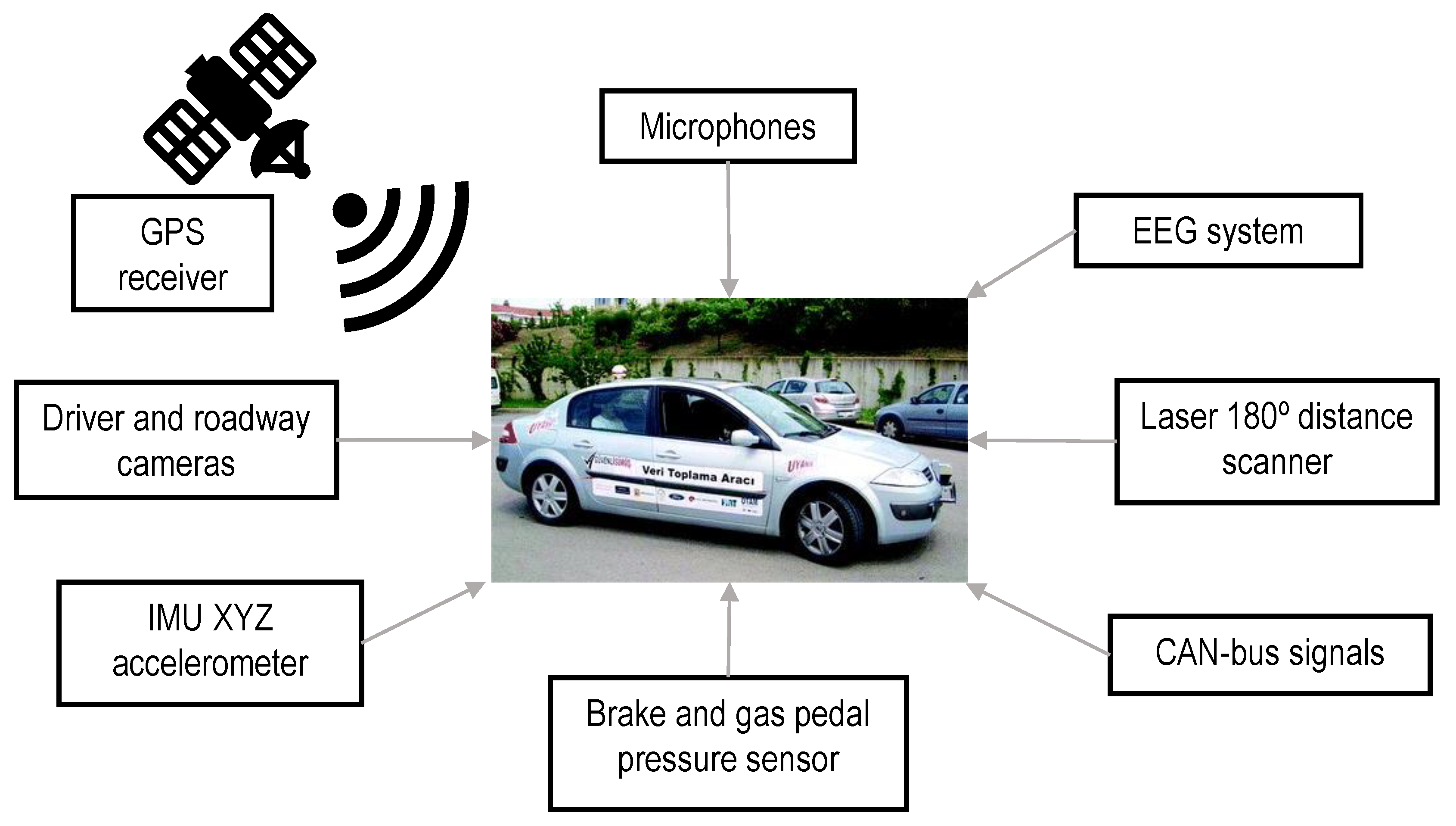
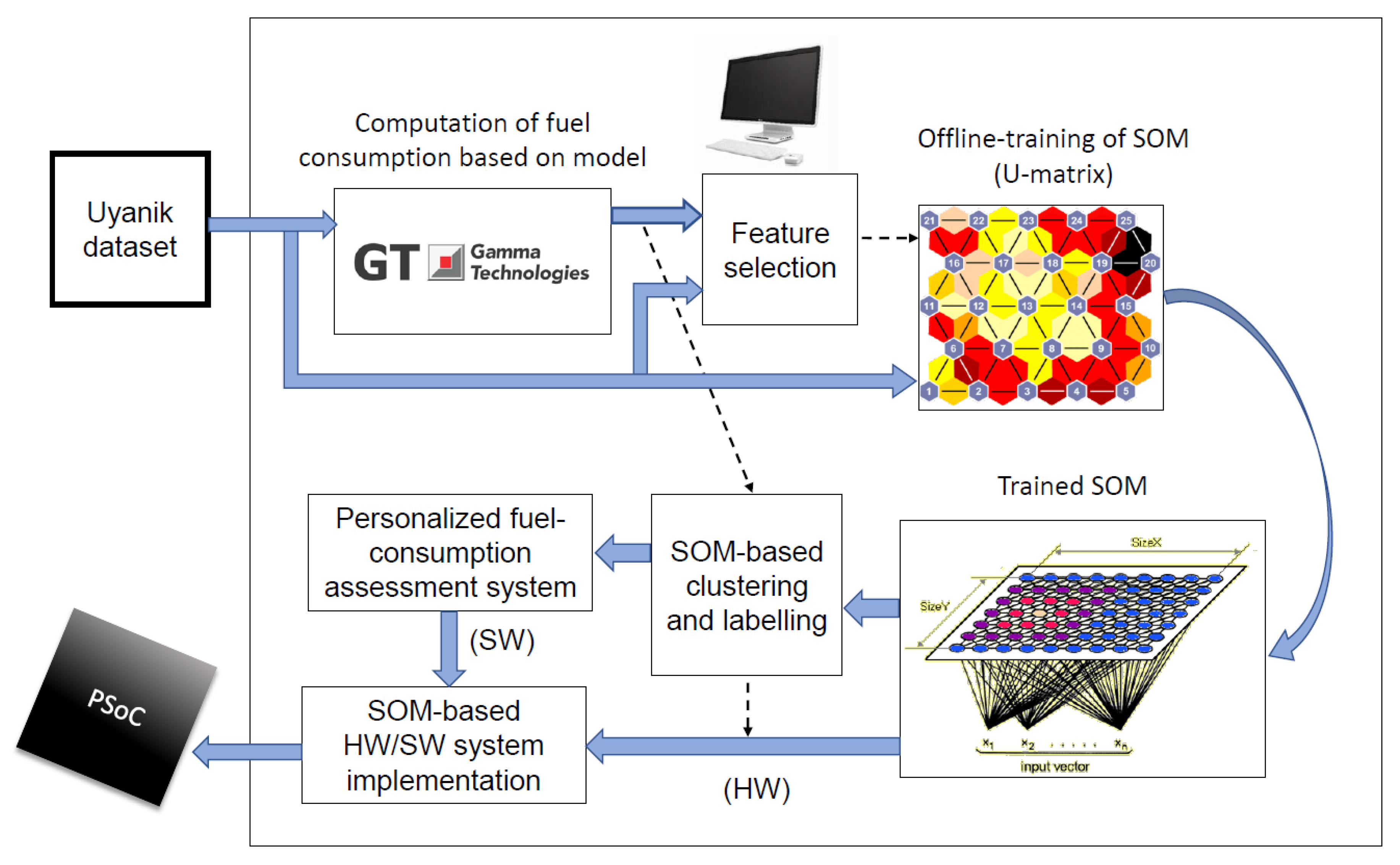
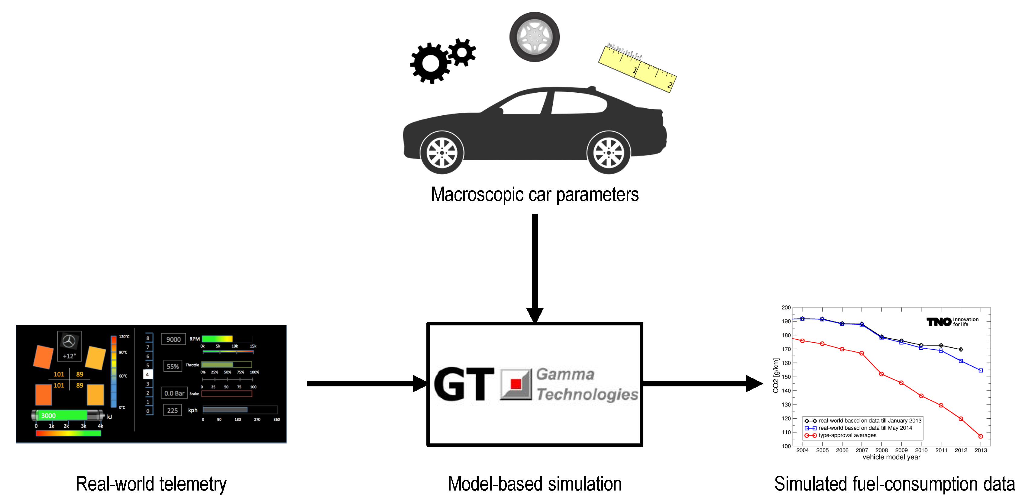
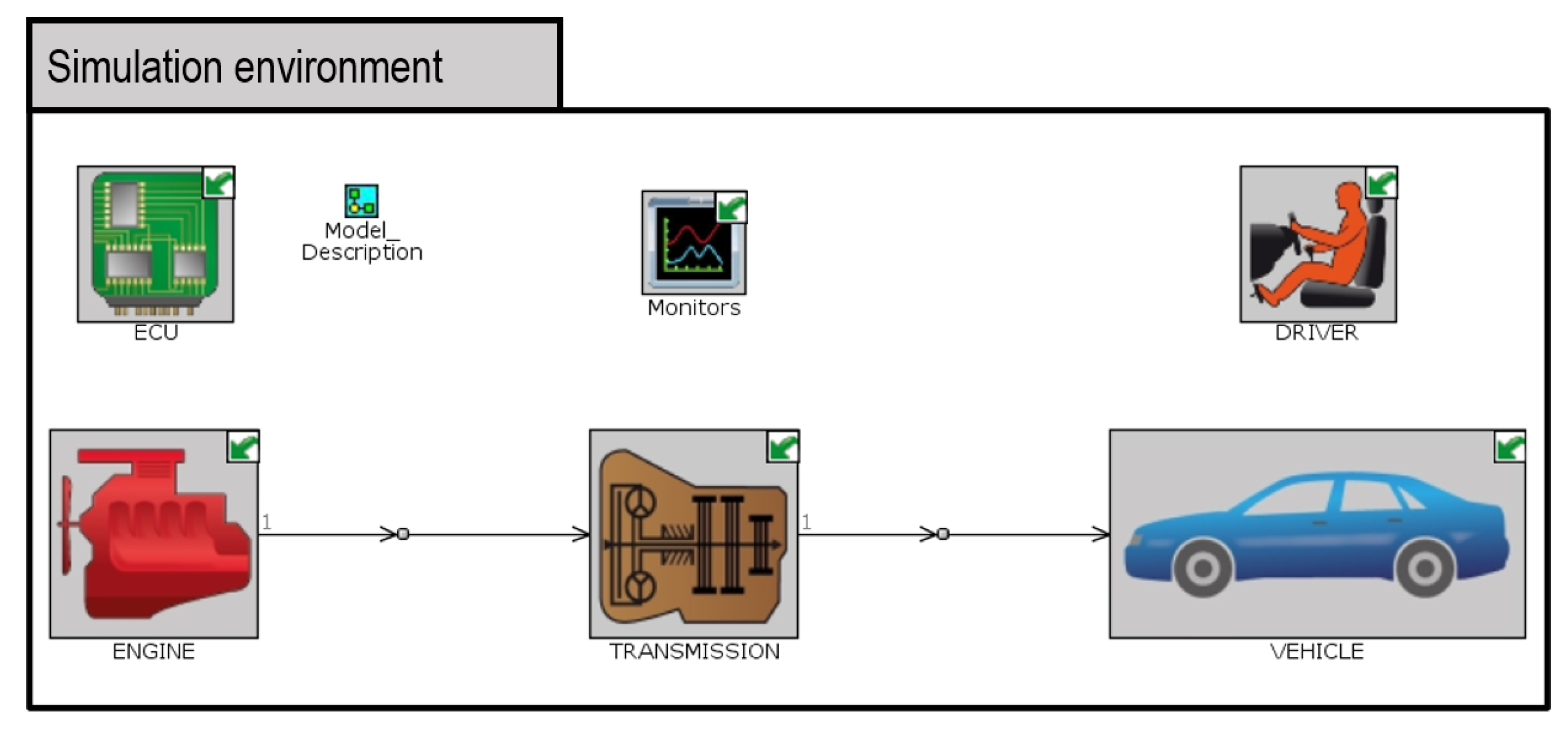
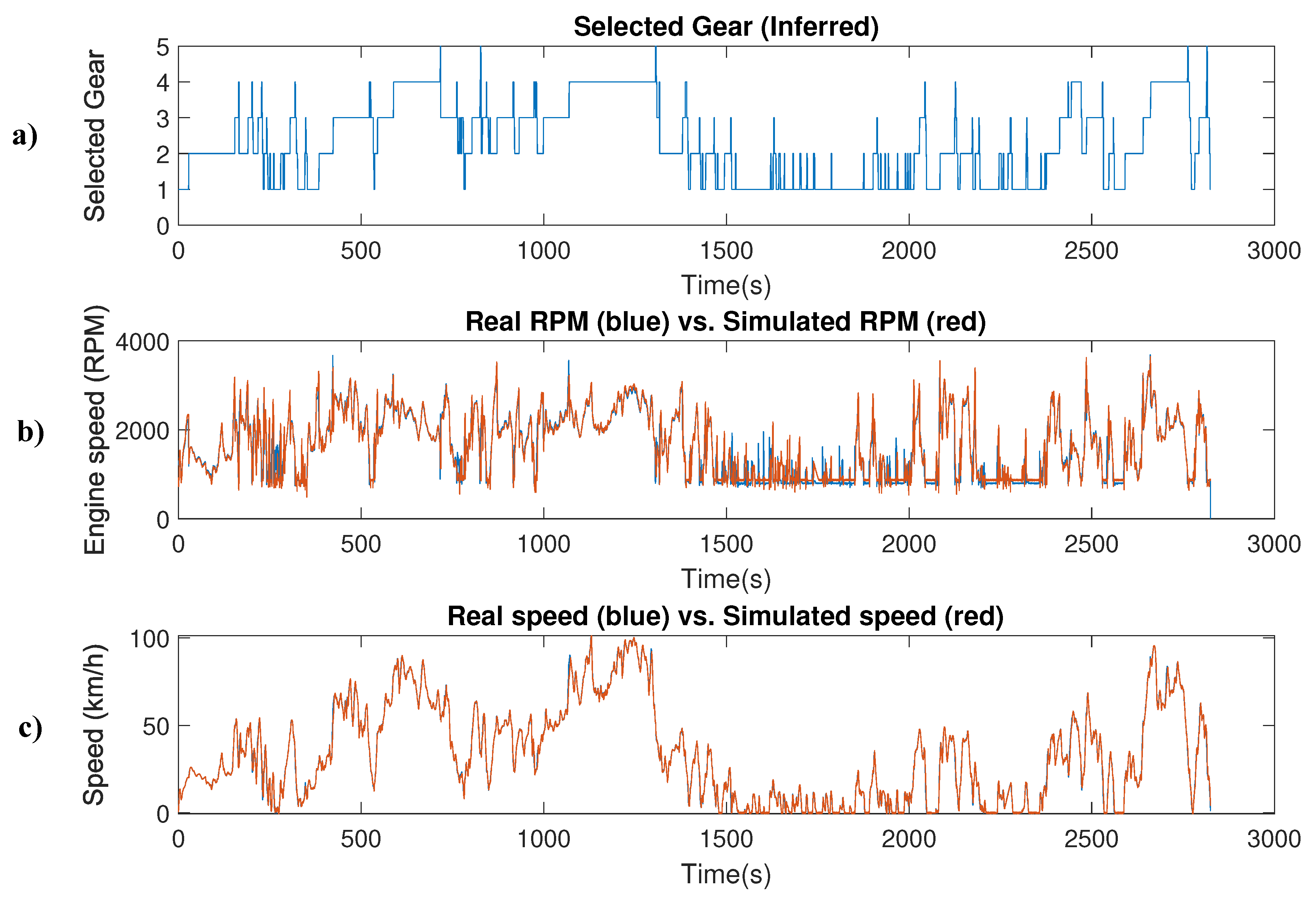
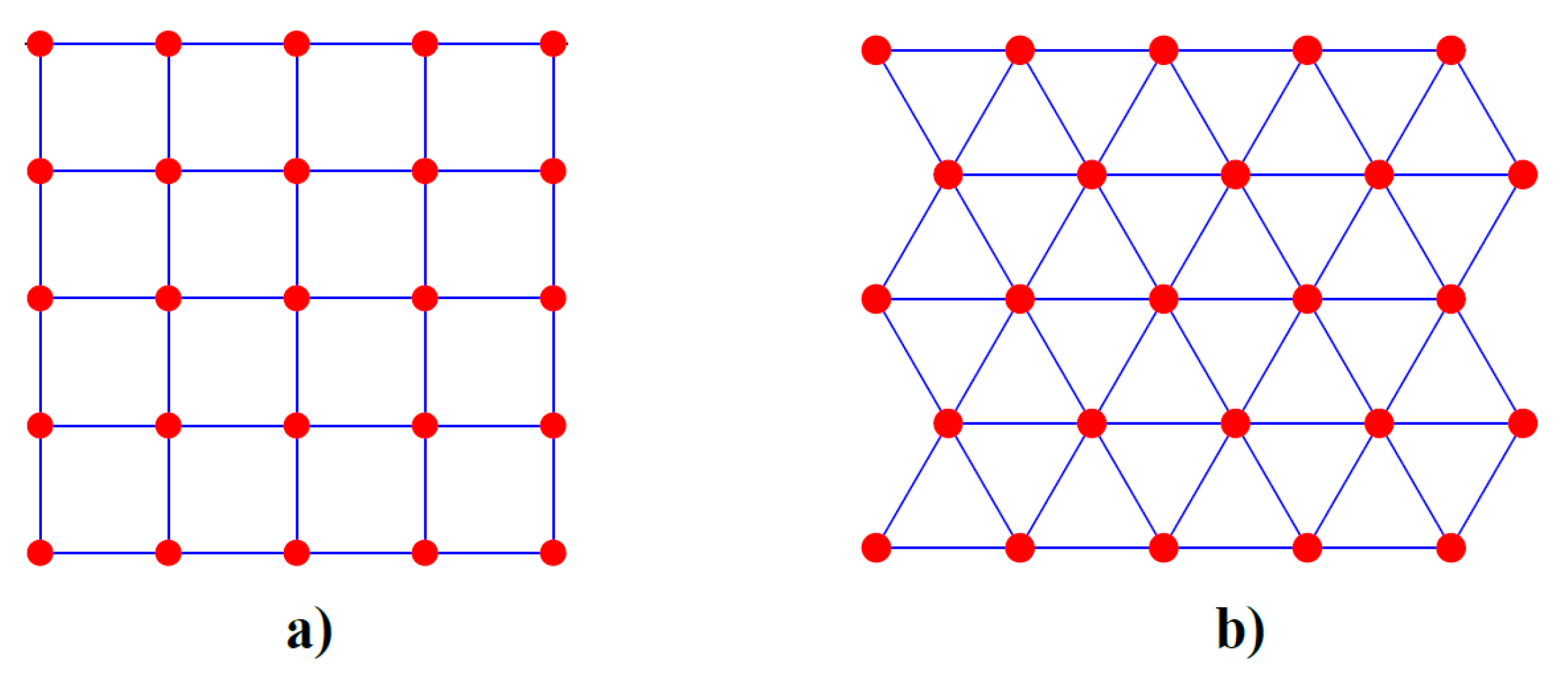
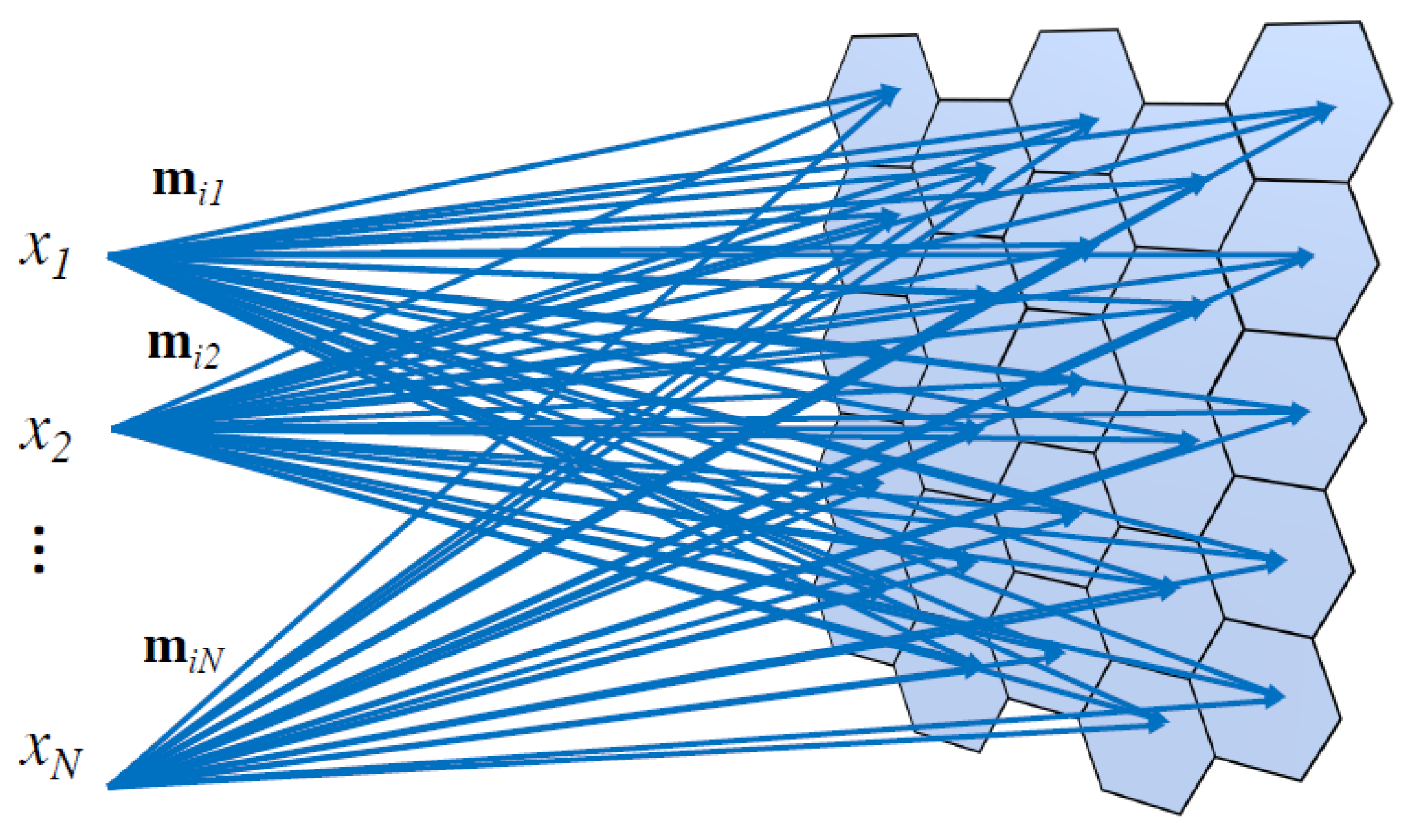
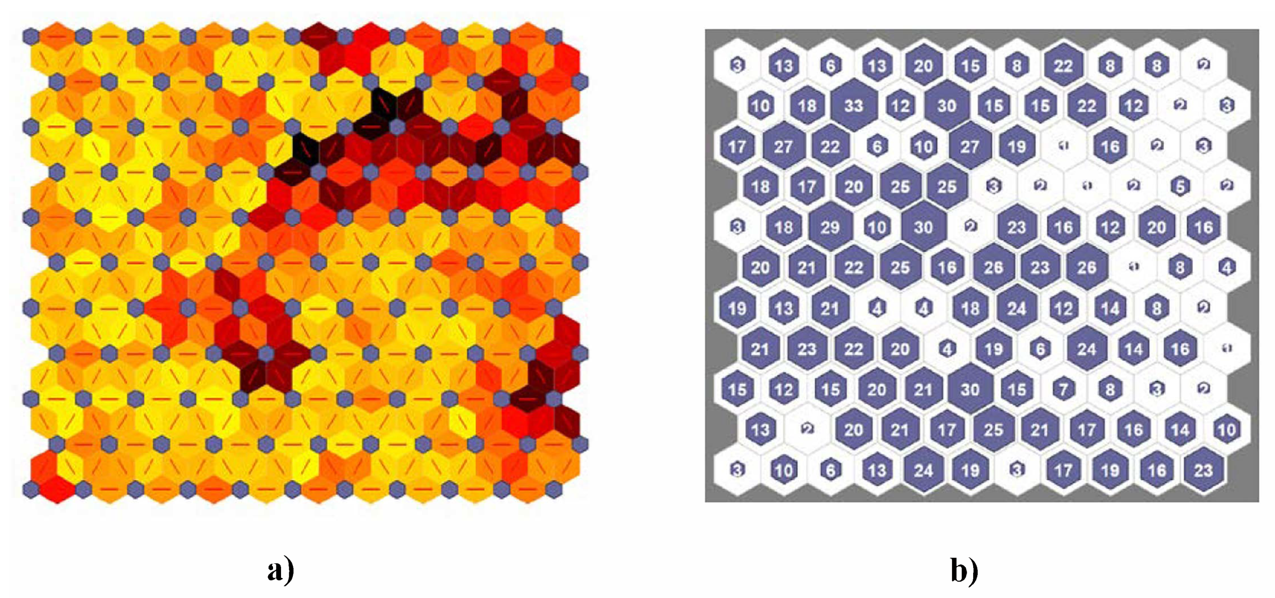
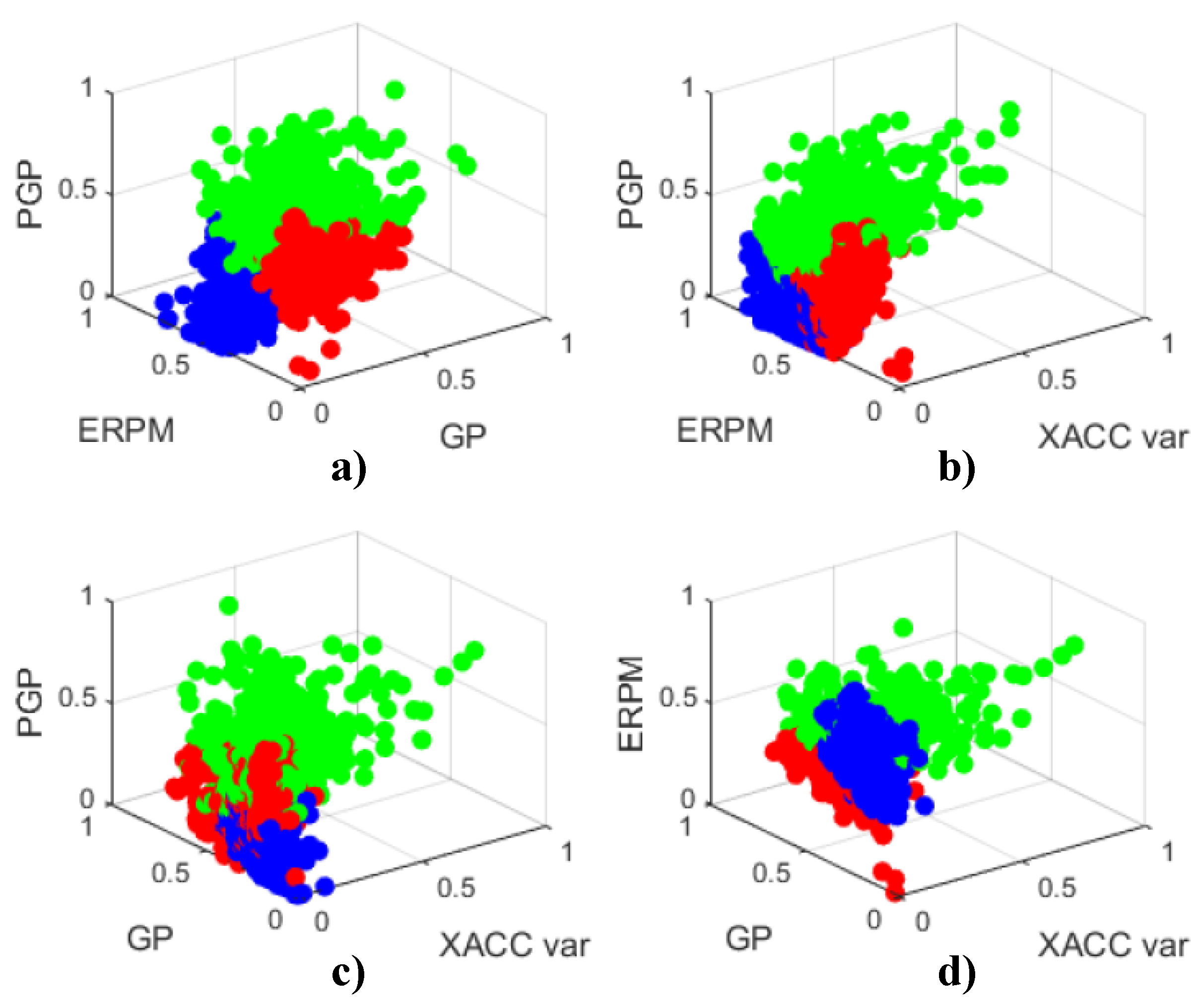
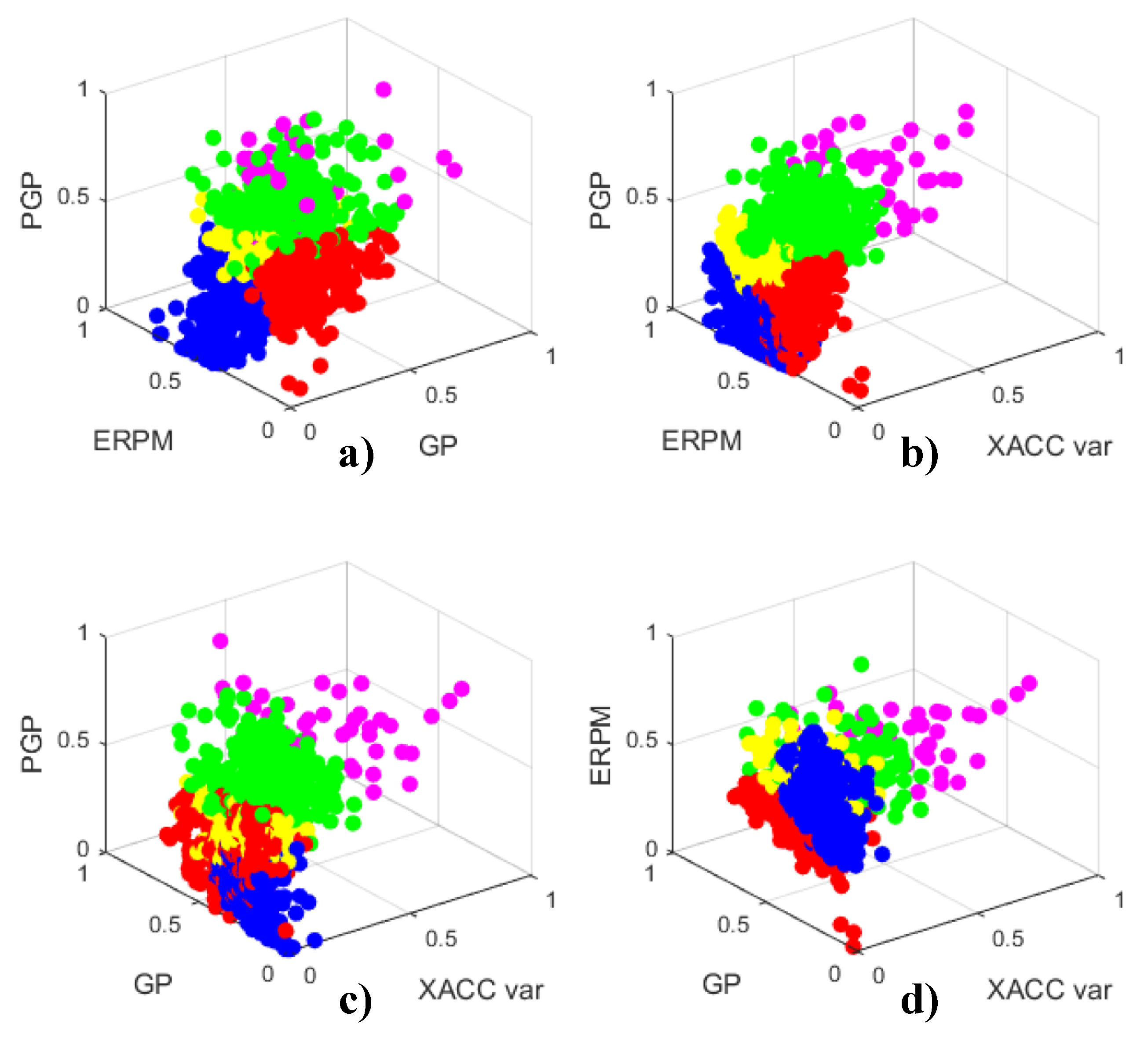
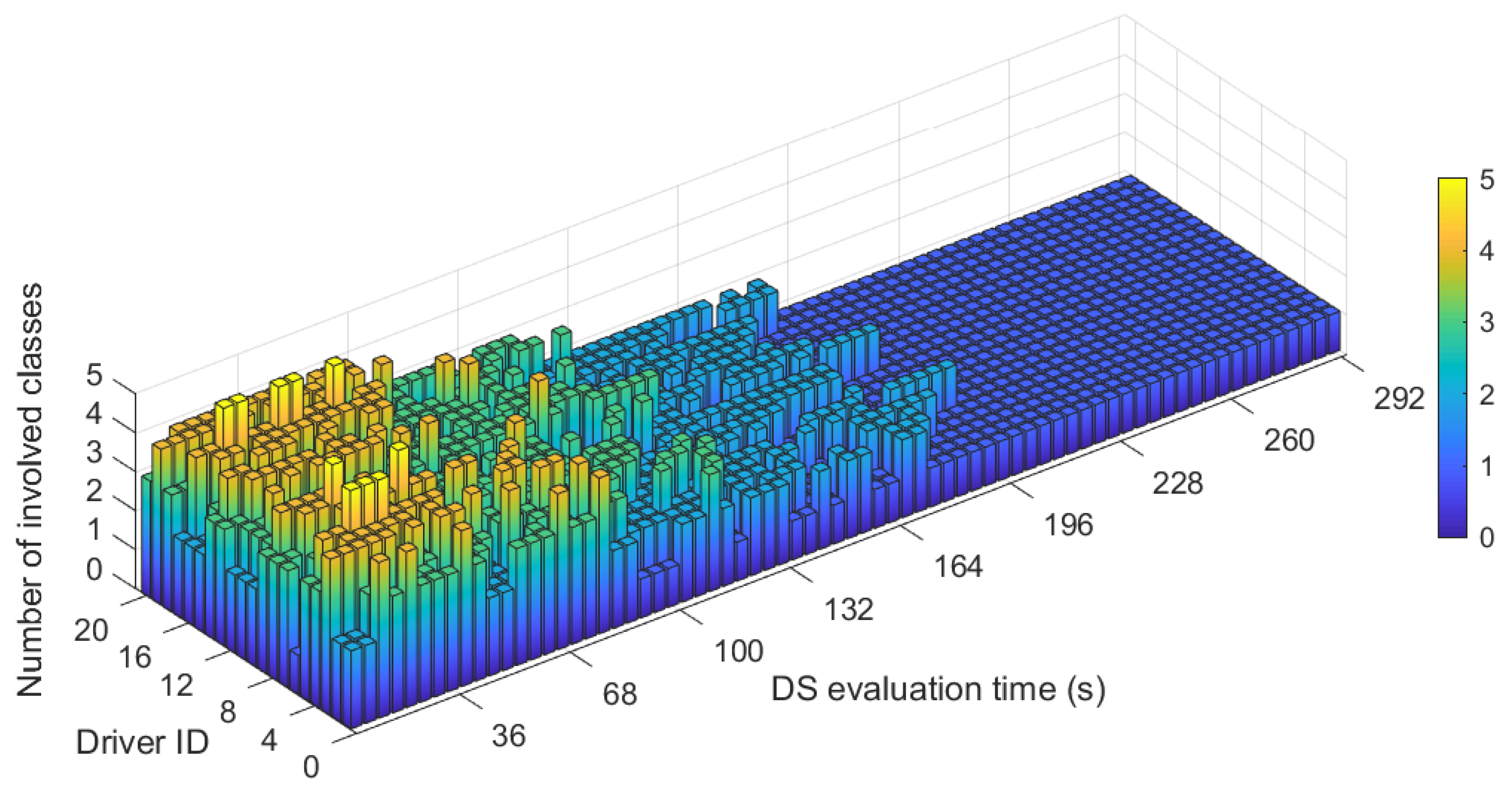
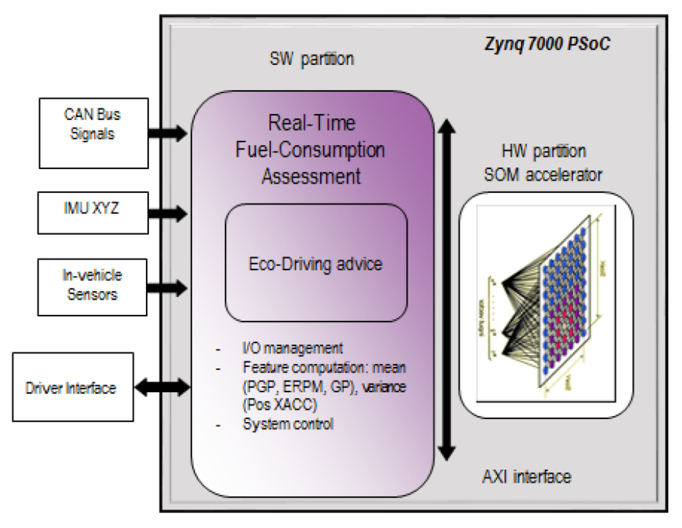
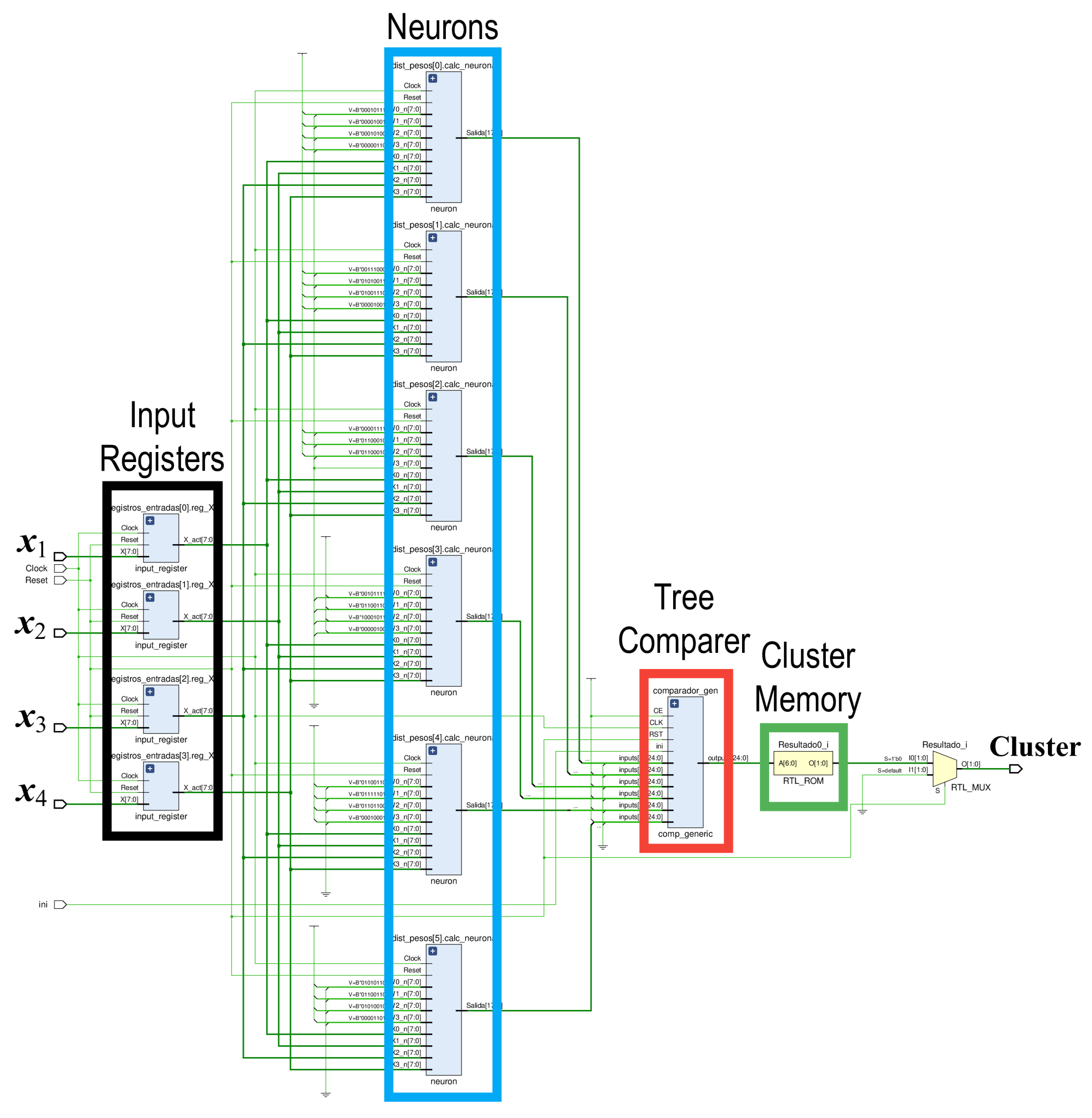
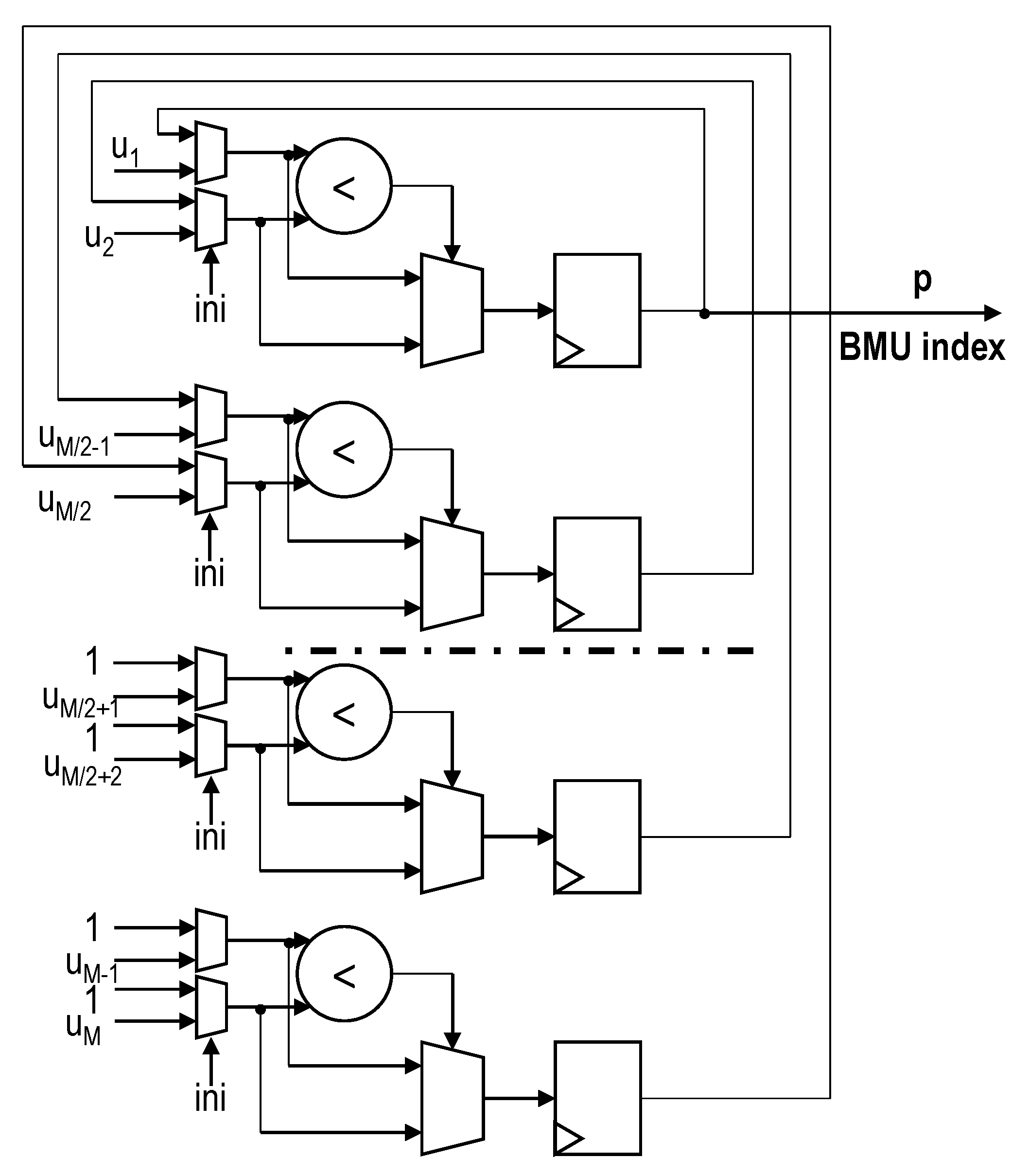
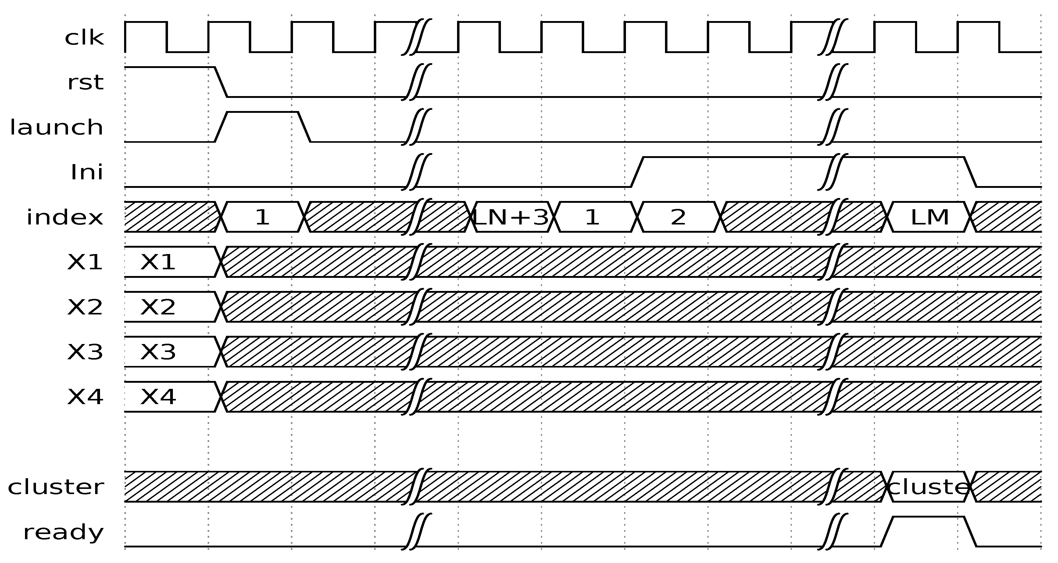
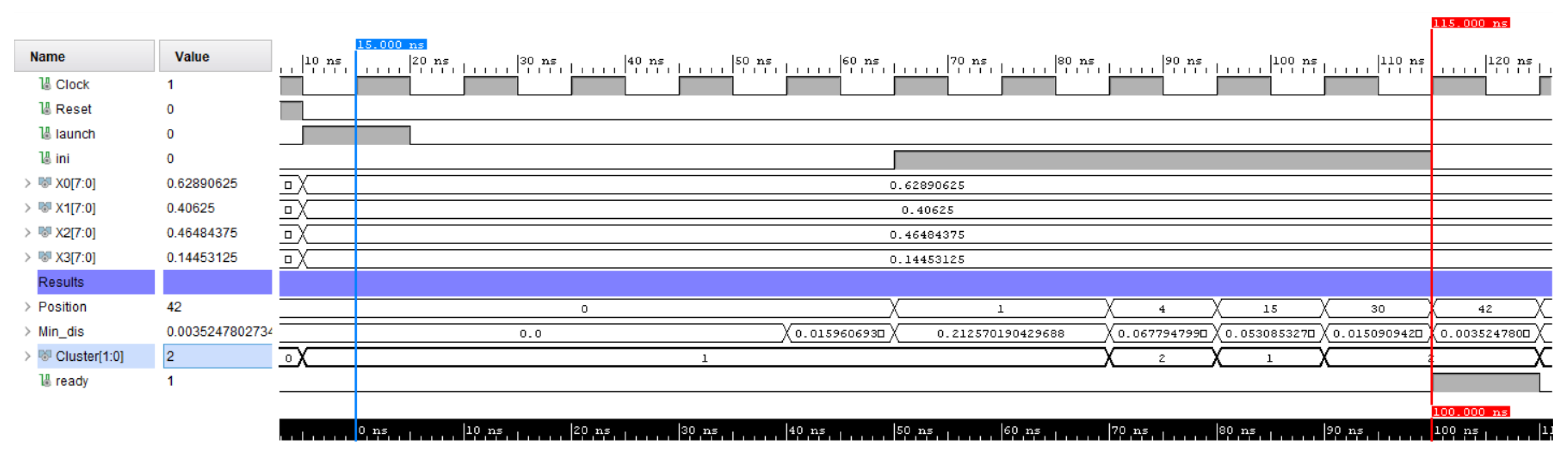
Table 1.
Significative variables of the Uyanik dataset [45].
Table 1.
Significative variables of the Uyanik dataset [45].
| Features | Signals (Time Series) |
|---|---|
| CAN bus | Steering wheel angle (SWA) |
| Steering wheel speed (SWS) | |
| Vehicle speed (VS) | |
| Percent gas pedal (PGP) | |
| Engine RPM (ERPM) | |
| Pressure sensors | Brake pedal pressure (BP) |
| Gas pedal pressure (GP) | |
| IMU unit | Roll rate (RR) |
| Pitch rate (PR) | |
| Yaw rate (YR) | |
| X axis accelerometer (XACC) | |
| Y axis accelerometer (YACC) | |
| Z axis accelerometer (ZACC) | |
| Laser | Distance to obstacle (d_90) |
| GPS | Coordinates (GPS) |
Table 2.
Driving behavior signals and Pearson correlation coefficients (PCCs) of fuel consumption with relevant features. Mean values and variances are computed using 8 s analysis windows.
Table 2.
Driving behavior signals and Pearson correlation coefficients (PCCs) of fuel consumption with relevant features. Mean values and variances are computed using 8 s analysis windows.
| Measurement Units | Signals (Time Series) | PCC: Mean | PCC: Variance |
|---|---|---|---|
| CAN-bus | Vehicle speed (VS) | 0.59 | 0.15 |
| Percent gas pedal (PGP) | 0.63 | 0.58 | |
| Engine RPM (ERPM) | 0.66 | 0.18 | |
| Pressure sensors | Brake pedal pressure (BP) | −0.35 | −0.23 |
| Gas pedal pressure (GP) | 0.52 | 0.20 | |
| IMU unit | Positive X axis acceleration (Pos XACC) | 0.32 | 0.25 |
| Negative X axis acceleration (Neg XACC) | −0.17 | −0.11 |
The boldface PCCs correspond to the strongest correlations.
Table 3.
Percentage of the route that each driver travels using different fuel-consumption driving styles (DSs) (three-cluster classification).
Table 3.
Percentage of the route that each driver travels using different fuel-consumption driving styles (DSs) (three-cluster classification).
| Driver | Very Low (%) | Low (%) | Medium-High (%) |
|---|---|---|---|
| D1 | 4.7 | 20.0 | 75.3 |
| D2 | 49.4 | 10.4 | 40.2 |
| D3 | 23.0 | 33.3 | 43.7 |
| D4 | 7.8 | 51.1 | 41.1 |
| D5 | 33.3 | 26.5 | 40.2 |
| D6 | 80.2 | 10.4 | 9.4 |
| D7 | 15.1 | 33.7 | 51.2 |
| D8 | 16.2 | 29.7 | 54.1 |
| D9 | 8.1 | 38.4 | 53.5 |
| D10 | 56.3 | 0 | 43.7 |
| D11 | 78.6 | 11.9 | 9.5 |
| D12 | 10.6 | 33.0 | 56.4 |
| D13 | 14.0 | 46.5 | 39.5 |
| D14 | 8.4 | 25.3 | 66.3 |
| D15 | 2.5 | 45.7 | 51.8 |
| D16 | 14.3 | 40.5 | 45.2 |
| D17 | 38.1 | 21.4 | 40.5 |
| D18 | 2.7 | 48.0 | 49.3 |
| D19 | 15.6 | 30.0 | 54.4 |
| D20 | 32.2 | 26.9 | 40.9 |
Table 4.
Fuel consumption (L/100km) parameters of the three-cluster classification.
| Cluster Label | Average Value | Variance | Maximum Value |
|---|---|---|---|
| Very low (red) | 2.76 | 1.02 | 6.66 |
| Low (blue) | 3.04 | 1.53 | 7.80 |
| Medium-High (green) | 5.15 | 3.34 | 12.6 |
Table 5.
Actions that are associated to the three-cluster classification.
| Current Cluster | Required Action |
|---|---|
| Very low (red) | Keep driving style |
| Low (blue) | Lower RPM/Switch to a higher gear |
| Medium-High (green) | Lower RPM/Keep gas steady/Lower PGP |
Table 6.
Fuel consumption (L/100km) parameters of the five-cluster classification.
| Cluster Label | Average Value | Variance | Maximum Value |
|---|---|---|---|
| Very low (red) | 2.75 | 1.04 | 6.66 |
| Low (blue) | 3.04 | 1.54 | 7.80 |
| Medium (yellow) | 4.44 | 2.21 | 10.1 |
| High (green) | 5.42 | 3.13 | 11.4 |
| Very high (magenta) | 7.81 | 5.38 | 12.5 |
Table 7.
Percentage of the route that each driver travels using different fuel-consumption DS (five-cluster classification).
Table 7.
Percentage of the route that each driver travels using different fuel-consumption DS (five-cluster classification).
| Driver | Very Low (%) | Low (%) | Medium (%) | High (%) | Very High (%) |
|---|---|---|---|---|---|
| D1 | 4.7 | 20.0 | 44.7 | 30.6 | 0 |
| D2 | 48.3 | 10.3 | 2.3 | 32.2 | 6.9 |
| D3 | 21.8 | 33.3 | 13.8 | 30.0 | 1.1 |
| D4 | 7.8 | 51.1 | 22.2 | 18.9 | 0 |
| D5 | 33.3 | 26.5 | 10.3 | 25.3 | 4.6 |
| D6 | 71.9 | 10.4 | 9.4 | 8.3 | 0 |
| D7 | 14.0 | 33.7 | 18.6 | 29.1 | 4.6 |
| D8 | 14.9 | 29.7 | 8.1 | 37.8 | 9.5 |
| D9 | 8.1 | 38.4 | 31.4 | 22.1 | 0 |
| D10 | 56.3 | 0 | 16.1 | 25.3 | 2.3 |
| D11 | 78.6 | 11.9 | 1.2 | 8.3 | 0 |
| D12 | 10.6 | 33.0 | 37.2 | 19.2 | 0 |
| D13 | 14.0 | 46.5 | 15.1 | 24.4 | 0 |
| D14 | 8.4 | 25.3 | 31.3 | 35.0 | 0 |
| D15 | 2.5 | 45.7 | 24.7 | 23.4 | 3.7 |
| D16 | 13.1 | 40.5 | 30.9 | 15.5 | 0 |
| D17 | 38.1 | 21.4 | 10.7 | 21.5 | 8.3 |
| D18 | 2.7 | 48.0 | 19.2 | 26.0 | 4.1 |
| D19 | 15.6 | 30.00 | 21.1 | 32.2 | 1.1 |
| D20 | 32.2 | 26.9 | 22.6 | 18.3 | 0 |
Table 8.
Actions associated to the five-cluster classification.
| Current Cluster | Required Action |
|---|---|
| Very low (red) | Keep driving style |
| Low (blue) | Lower RPM/Switch to a higher gear |
| Medium (yellow) | Lower RPM/Operate gas softly |
| High (green) | Lower PGP/Lower RPM |
| Very high (magenta) | Lower PGP/Keep gas steady |
Table 9.
Expected fuel-consumption reduction between contiguous clusters.
| Current Cluster | Target Cluster | Reduction (%) |
|---|---|---|
| Low | Very low | 9.5 |
| Medium | Low | 31.5 |
| High | Medium | 18.1 |
Table 10.
Post-implementation resources report (Xilinx XC7Z045-2FFG900).
| Resource | Utilization | Available | % Used |
|---|---|---|---|
| LUT | 21 107 | 218 600 | 9.66 |
| Flip-flops | 13 337 | 437 200 | 3.05 |
© 2020 by the authors. Licensee MDPI, Basel, Switzerland. This article is an open access article distributed under the terms and conditions of the Creative Commons Attribution (CC BY) license (http://creativecommons.org/licenses/by/4.0/).
Share and Cite
MDPI and ACS Style
Mata-Carballeira, Ó.; Díaz-Rodríguez, M.; del Campo, I.; Martínez, V. An Intelligent System-on-a-Chip for a Real-Time Assessment of Fuel Consumption to Promote Eco-Driving. Appl. Sci. 2020, 10, 6549. https://doi.org/10.3390/app10186549
AMA Style
Mata-Carballeira Ó, Díaz-Rodríguez M, del Campo I, Martínez V. An Intelligent System-on-a-Chip for a Real-Time Assessment of Fuel Consumption to Promote Eco-Driving. Applied Sciences. 2020; 10(18):6549. https://doi.org/10.3390/app10186549
Chicago/Turabian StyleMata-Carballeira, Óscar, Mikel Díaz-Rodríguez, Inés del Campo, and Victoria Martínez. 2020. "An Intelligent System-on-a-Chip for a Real-Time Assessment of Fuel Consumption to Promote Eco-Driving" Applied Sciences 10, no. 18: 6549. https://doi.org/10.3390/app10186549
Note that from the first issue of 2016, this journal uses article numbers instead of page numbers. See further details here.