Optimal Containment Control Strategy of the Second Phase of the COVID-19 Lockdown in Morocco

Abstract

This work investigates the optimal control of the second phase of the COVID-19 lockdown in Morocco. The model consists of susceptible, exposed, infected, recovered, and quarantine compartments (SEIRQD model), where we take into account contact tracing, social distancing, quarantine, and treatment measures during the nationwide lockdown in Morocco. First, we present different components of the model and their interactions. Second, to validate our model, the nonlinear least-squares method is used to estimate the model’s parameters by fitting the model outcomes to real data of the COVID-19 in Morocco. Next, to investigate the impact of optimal control strategies on this pandemic in the country. We also give numerical simulations to illustrate and compare the obtained results with the actual situation in Morocco.

1. Introduction

On 31 December 2019, a novel coronavirus named (COVID-19) was detected in Wuhan City, Hubei Province of China [1]. Human coronaviruses chiefly cause respiratory infections that can be a simple mild cold or a severe and sometimes fatal lung disease. The speed of the worldwide spread of the virus is unprecedented. The human mobility means that almost all countries are now infected [2]. As there is currently no vaccine available to protect against COVID-19 and no specific drug treatment [3], the government in each country has adopted extreme measures to mitigate the outbreak, suspending all public traffic within the cities, and closing all inbound and outbound transportation. Therefore, several researchers have studied a mathematical model to estimate the transmissibility [4,5,6,7,8], and the dynamic of the transmission of the virus and the calculation of the basic reproduction number ${\mathcal{R}}_0$ [9,10].

Chen et al. [5] studied a mathematical model describing the transmissibility of SARS-CoV-2, by developing an RP transmission model, which takes into account the reservoir-to-person and person-to-person pathways of SARS-CoV-2. Zhao et al. [10] modeled the epidemic curve of the 2019-nCoV cases’ time series, in mainland China, through the exponential growth. They demonstrated that changes in reporting rate substantially affect estimates of the basic reproduction number ${\mathcal{R}}_0$. Lina et al. [6] have investigated a model for the COVID-19 outbreak in Wuhan with the consideration of individual behavioral reactions and governmental actions, e.g., holiday extension, travel restriction, hospitalization, and quarantine.

Liu et al. [7] have proposed a quarantine-susceptible, exposed, infection-resistant model, which considers the strict quarantine imposed in almost all of China to contain the epidemic. They estimated the model’s parameters with the statistical method and stochastic simulation. In [11], the authors have presented a new mathematical model describing the evolution of COVID-19 in countries under a national lockdown and studied the impact of staying at home on the pandemic spread, especially in Morocco and Italy, in which they have considered two new classes of people: those who underestimated the quarantine and left their home, called the partially controlled people, and those who respected the national quarantine by staying at home, called the totally controlled people.

In this paper, we consider a new COVID-19 epidemic discrete mathematical model that considers the strict quarantine measures imposed in almost all countries to resist the epidemic. We sought the optimal strategies to minimize the number of exposed and infected people. We looked at optimal strategies to reduce the infected and susceptible contact by adopting the quarantine strategy for the infection and choosing containment throughout the country. To achieve this purpose, we looked at optimal control strategies that represent awareness campaigns that aim to introduce health measures to protect individuals from being infected by the virus and the security campaigns and health measures to prevent individuals’ movement. We set the characterization of optimal control strategies, and we give the explicit expression of the optimal controls by using Pontryagin’s maximum principle.

The paper is organized as follows. In Section 2.1, we present a description of the COVID-19 discrete mathematical model that describes the dynamics of the COVID-19 disease propagation and which includes contact tracing, quarantine, and treatment during the strict national closure in the whole of a country to resist the epidemic. In Section 2.2, we estimate the parameters to validate the proposed model by fitting the model outputs to real data. In Section 2.3, we present the optimal control problem for the proposed model, and we characterize these optimal controls using Pontryagin’s maximum principle in discrete time. Numerical simulations and comparison of the different strategies are given in Section 3. Finally, we conclude the paper in Section 4.

2. Materials and Methods

2.1. Model Description

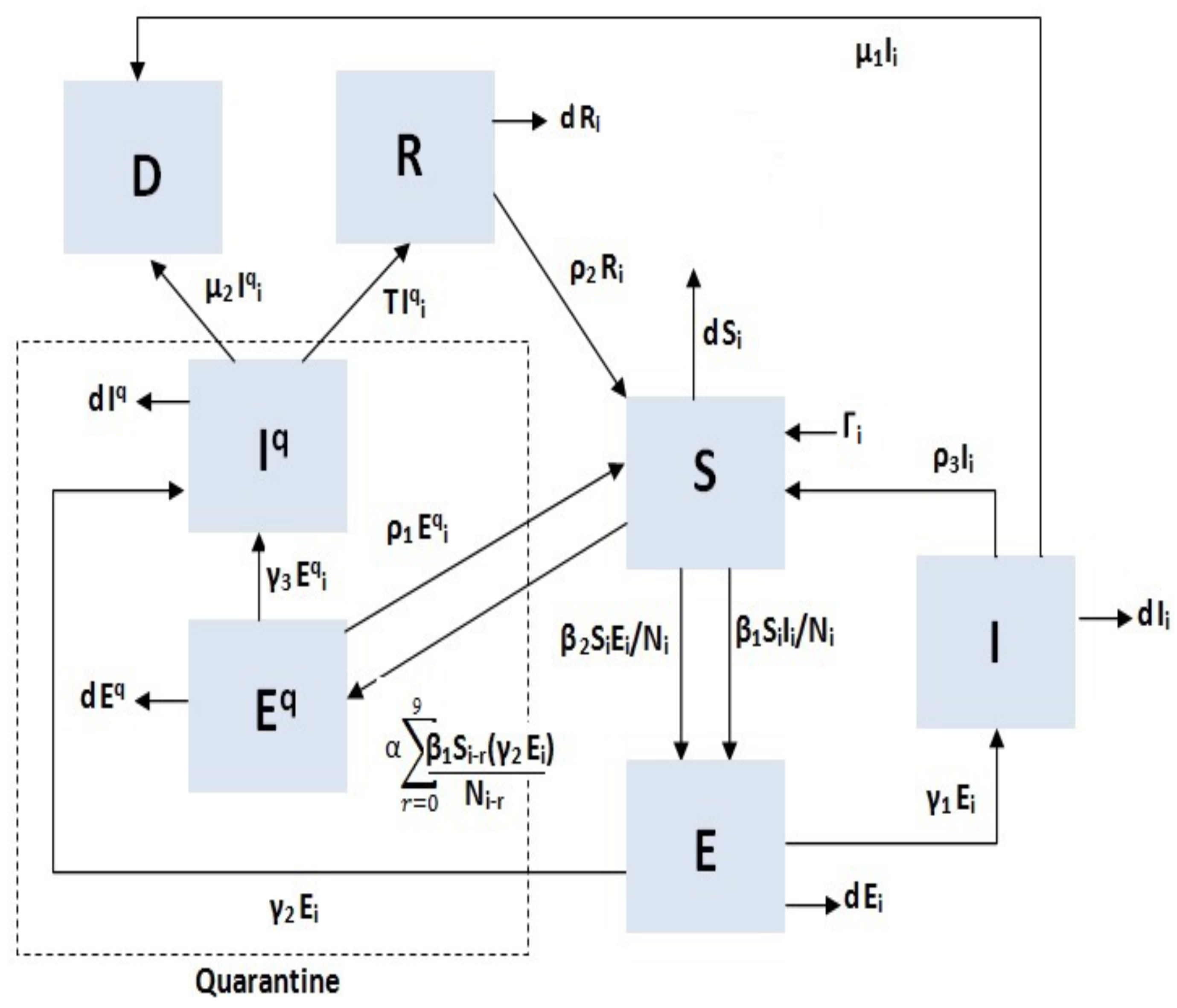
In this paper, we propose a discrete-time SEIRQD-type COVID-19 epidemic model. We take into account that the exposed are asymptomatic, which means that they are also infectious. The model is describe by the following discrete system

$$\begin{array}{ccc}{S}_{i+1}& =& {\mathsf{\Gamma }}_i+S_i+{\rho }_1{E}_i^q+{\rho }_2{R}_i+{\rho }_3{I}_i-{\beta }_1(1-u_i)\frac{S_i{I}_i}{N_i}-{\beta }_2(1-v_i)\frac{S_i{E}_i}{N_i}-\alpha {\displaystyle \sum _{r=0}^9}\frac{{\beta }_1{S}_{i-r}\left({\gamma }_2{E}_i\right)}{N_{i-r}}-d{S}_i;\hfill \\ E_{i+1}& =& E_i+{\beta }_1(1-u_i)\frac{S_i{I}_i}{N_i}+{\beta }_2(1-v_i)\frac{S_i{E}_i}{N_i}-({\gamma }_1+{\gamma }_2+d)E_i;\hfill \\ I_{i+1}& =& I_i+{\gamma }_1{E}_i-({\mu }_1+{\rho }_3+d)I_i;\hfill \\ R_{i+1}& =& R_i+T{I}_i^q-({\rho }_2+d)R_i;\hfill \\ E_{i+1}^q& =& E_i^q+\alpha {\displaystyle \sum _{r=0}^9}\frac{{\beta }_1{S}_{i-r}\left({\gamma }_2{E}_i\right)}{N_{i-r}}-({\rho }_1+{\gamma }_3+d)E_i^q;\hfill \\ I_{i+1}^q& =& I_i^q+{\gamma }_2{E}_i+{\gamma }_3{E}_i^q-(T+{\mu }_2+d)I_i^q;\hfill \\ D_{i+1}& =& D_i+{\mu }_2{I}_i^q+{\mu }_1{I}_i;\hfill \end{array}$$

(1)

subject to non-negative initial conditions. $S_i$, $E_i$, $I_i$, $R_i$, and $D_i$ denote the number of susceptible, exposed, infectious, recovered, and dead persons. $E_i^q$ and $I_i^q$ denote the number of exposed and infectious persons in quarantine. In such a SEIRQD-model type of the COVID-19, $N_i$ is the total population size, the incubation period is estimated to be 7 days and the infectious period of the virus is estimated as 10 days.

A susceptible person can infected by contacting either an infected person or an exposed (asymptomatic) person. The number of these contacts is ${\beta }_1\frac{S_i{I}_i}{N_i}+{\beta }_2\frac{S_i{E}_i}{N_i}$.

The control strategy that was introduced into this system aims to reduce contact between susceptible people and infected or exposed people.

For a period of 10 days of virus incubation, the symptoms might appear in a portion of $E_i$ individuals. Hence, a fraction of these individuals, ${\gamma }_1{E}_i$, will choose not to be hospitalized, as their symptoms are mild and can be treated at home. We also assume that infected person become infected again with the rate ${\rho }_3{I}_i$. There are cases of infected people who died, and their autopsy confirmed COVID-19 as cause of death; therefore, a fraction ${\mu }_1{I}_i$ will be added to the number of deceased caused by COVID-19. The other fraction of the asymptomatic ${\gamma }_2{E}_i$ is hospitalized and put under medical care. Once a person is infected and hospitalized, the health service tries to trace the people who contacted the infected person during the 10 days of the virus incubation period. The individuals that are traced will be quarantined and placed under medical care. ${\displaystyle \sum _{r=0}^9}\frac{S_{i-r}\left({\gamma }_2{E}_i\right)}{N_{i-r}}$ is the total number of people who were in contact with infected people before being quarantined. The ${\gamma }_3{E}_i^q$ of cases will have symptoms and will be placed under medical surveillance, or they will have to get medical care if their symptoms are mild. The contacts who tested negative, after an observation period, find themselves newly susceptible with a ${\rho }_1{E}_i^q$ rate. Among these infected cases, a number of ${\mu }_2{I}_i^q$ will have died and a number of $T{I}_i^q$ will be recovered. The recovered people do not have immunity from the COVID-19; therefore, they may be susceptible again. The birth rate ${\mathsf{\Gamma }}_i$ is $16.5\%$ of the total population [12] and the natural mortality rate d is equal to $5.8\%$.

All the above parameters are assumed to be non-negative and defined in

Table 1. The description of parameters used for the definition of SEIRQD model type of COVID-19 (1).

Parameter	Description
${\mathsf{\Gamma }}_i$	the number of people born at the moment i.
${\beta }_1$	The transmission rate from I to S.
${\beta }_2$	The transmission rate from E to S.
$\alpha$	The rate that a quarantined individual is exposed to infection.
${\gamma }_1$	rate changes of an exposed state E to infected state I.
${\gamma }_2$	rate changes of an exposed state E to infected state $I^q$.
${\gamma }_3$	rate changes of an exposed state $E^q$ to infected state $I^q$.
${\mu }_1$	rate changes of an infected state I to susceptible state S.
${\mu }_2$	rate changes of an infected state $I^q$ to death state D.
${\rho }_1$	rate changes of an exposed state $E^q$ to susceptible state S.
${\rho }_2$	rate changes of an cure state R to susceptible state S.
${\rho }_3$	rate changes of an infected state I to susceptible state S.
T	rate changes of an infected state $I^q$ to the cure state R.
u	control measures for reduce contact between susceptible and infected persons.
v	control measures for reduce contact between susceptible and exposed persons.
d	The death rate of people.

. Schematically, the flow between compartments is represented in Figure 1.

2.2. Estimation of the Parameters

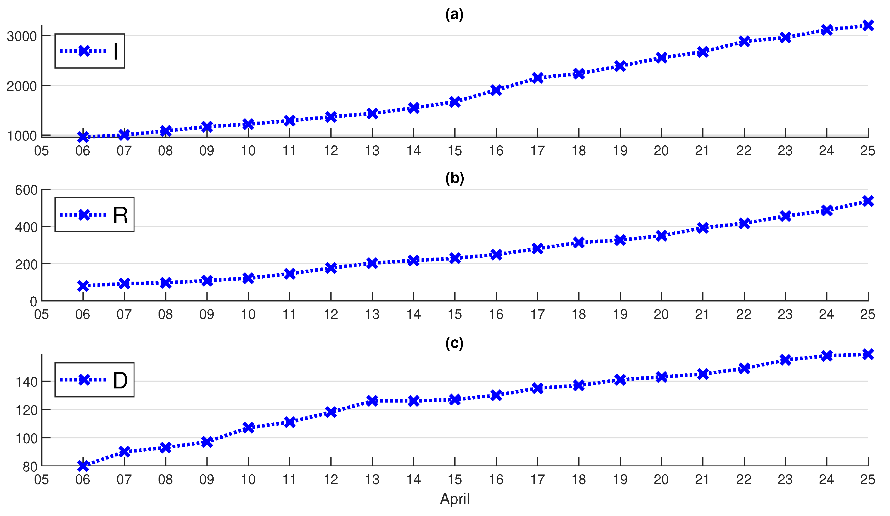
Our study focuses on the second phase of national lockdown in Morocco, from 6 April to 25 April, which is the time when wearing facial masks become obligatory, social distancing was implemented in all public places and many tests were carried out, as depicted in Figure 2. This is due to the rapid response of the Moroccan government, applying the nationwide quarantine after only 63 cases and two deaths on 20 March.

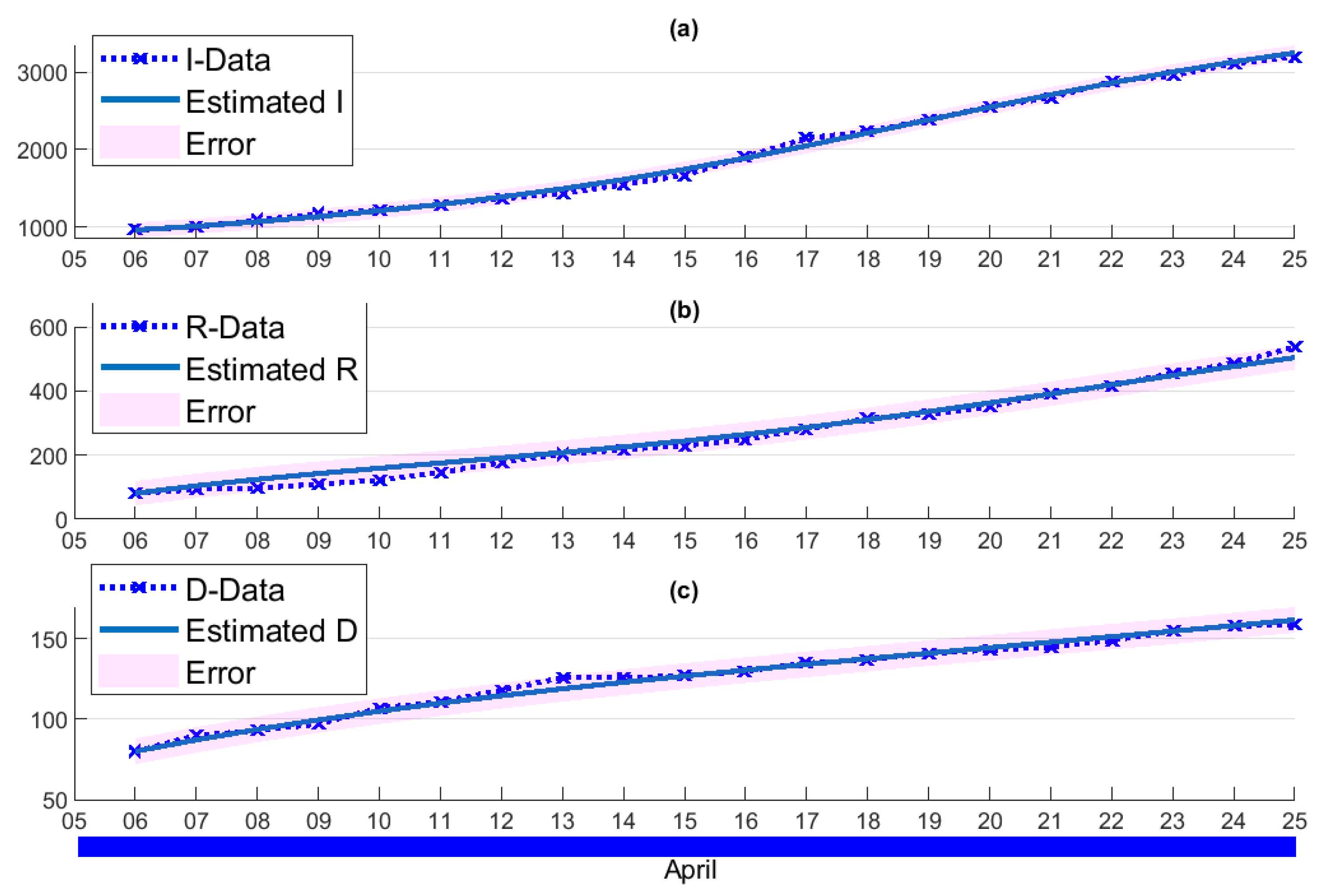
To verify the validity of our model, we used nonlinear least-squares regression to fit the model to actual data. Therefore, the following process was followed for parameter estimation:

The system of difference equations is solved numerically, the initial values chosen for the parameters, and the initial state variables of

Table 2. Estimated parameters’ values and the initial conditions for SEIRQD Model.

Parameter	Value
${\mathsf{\Gamma }}_i$	$\delta N_i$
${\beta }_1$	0.892559835359739
${\beta }_2$	0.0268308310475789
$\alpha$	0.899989478657192
${\gamma }_1$	4.38815800908638 $\times {10}^{-6}$
${\gamma }_2$	0.028964892404635
${\gamma }_3$	0.0448799035924354
${\mu }_1$	0.0063390258125248
${\mu }_2$	0.000866774799367013
T	0.0438013932330731
u	0.000293106579352138
v	0.529909144905706
${\rho }_1$	4.5368569540136 $\times {10}^{-7}$
${\rho }_2$	0.171682998125492
${\rho }_3$	0.0465276743678475
d	0.0586180610122414
$S_0$	34,500,000
$E_0$	2000
$I_0$	1000
$R_0$	81
$E_0^q$	2000
$I_0^q$	959
$D_0$	80

. The results of the model are compared with the field data, and the Levenberg–Marquardt optimization algorithm defines a new set of parameter values, with the results of the model better suited to field data. After determining the values of the new parameters with this optimizer, the system of difference equations is solved numerically using the value of these new parameters, and the results of the model are again compared with the field data. This iteration process continues between the updating of the parameters and the numerical solutions of a system of difference equations, using iterative diagrams until the criteria for convergence of the parameters are fulfilled. In this process of estimating the parameters, around one thousand values, are chosen using a random process for each of the parameters to be estimated.

Due to the effectiveness of large-scale awareness programs in the whole country, it is easy to identify infected people by their symptoms. Thus, the cases that were not reported are almost non-existent in the midst of the efforts exerted by the authorities and the different control strategies. This is why we can see that the parameter ${\gamma }_1$ has a small value. We can also see the percentage of people sent home to take care of themselves, that is to say, ${\rho }_1$, which means that the space for new patients allocated by the Moroccan authorities is very sufficient and there is still space available.

In Figure 3, we can see that our model fits correctly with the real data of Morocco, especially the data of infected and dead cases, see the sub-figures (a) and (c). In (a), (b), and (c) we can see the estimation of the I function, R function, and the D function, respectively, where there are some errors plotted with the filled area.

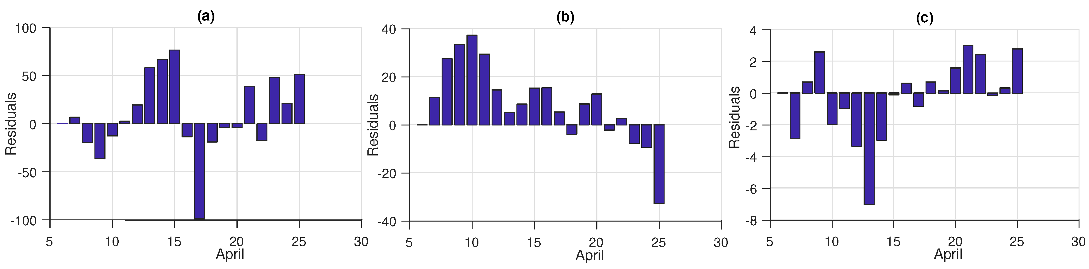
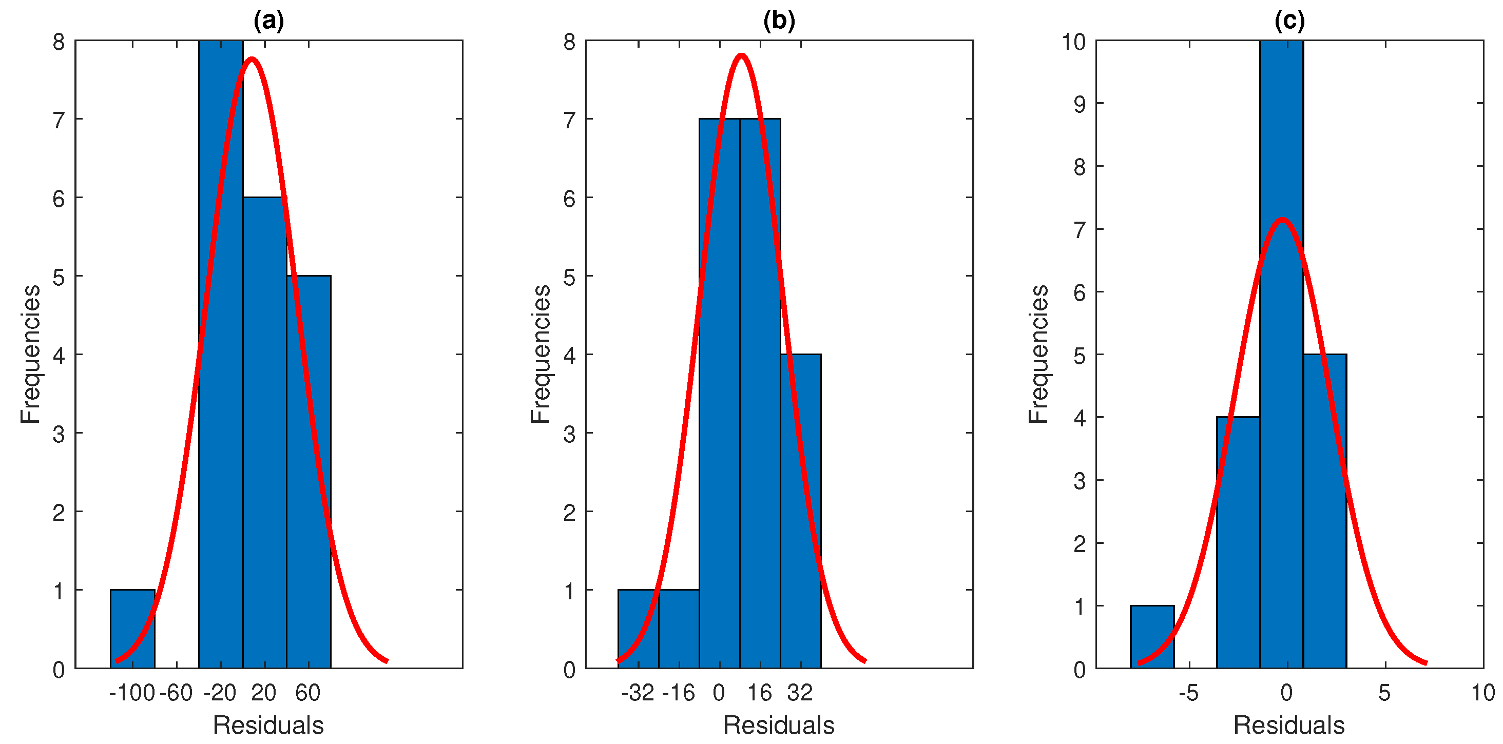
Because the residuals needs to be determined numerically, we examined the accuracy of the normality of the estimation of the parameters. In order to carry out this examination, we generated the residuals of the infected, recovered and dead populations for data of Morocco. First, residuals are plotted in Figure 4, where we can see ranges of $I_k-I_k^{data}$ in (a) and $R_k-R_k^{data}$ in (b) and $D_k-D_k^{data}$ in (c). It can be seen from the figure that residuals of the infected population are in the range $[-50,50]$, and residuals of the recovered population are in the range $[-30,50]$, while residuals of the dead population are in the range $[-6,6]$. Second, Figure 5 displays the corresponding histograms of $I_k-I_k^{data}$ in (a) and $R_k-R_k^{data}$ in (b) and $D_k-D_k^{data}$ in (c) for the estimation of the parameters for Morocco with their corresponding normal distributions.

In order to make valid inferences during regression analysis, it is necessary to check the assumptions, in order to be able to trust the results. One of the most useful assumptions for regression analysis is that the residuals are normally distributed. It can be seen from these figures that the residuals follow a normal distribution, furthermore, they remain within small ranges, thus the estimated parameters are reliable and correctly predict the observed data of Morocco, especially the number of infections and deaths.

The objective of this part of the article is not to predict what will happen in the coming months, but to validate the proposed model by fitting the model’s outputs to real data. Therefore, our next objective is to suggest optimal control strategies to make the national lockdown more effective in reducing new infections and saving more lives.

2.3. The Optimal Control

During this pandemic, all affected countries over the world adopted national lockdowns, social distancing, and quarantines. The Moroccan authorities started the lockdown on the 20th March, when the infections reached 63 cases, which is considered early compared to some countries that intervened after huge numbers of COVID-19 cases were recorded. Optimal control techniques are of great use in developing optimal strategies to control various kinds of diseases. To solve the challenges in obtaining an optimal control strategy, we consider the variables $(u_i,v_i,T_i)\in {\mathcal{U}}_{ad}^T$. $\left(u_i\right)$ to be control measures for reducing contact between susceptible and infectious person per unit of time, by providing people with all the necessary information to identify symptoms of a suspected case and the necessary precautions to avoid infection, $\left(v_i\right)$, which include control measures for reducing contact between susceptible and exposed persons per unit of time by imposing social distancing, self-isolation and not leaving home unless absolutely necessary, and wearing masks. $T_i$ is the treatment per unit of time. The set ${\mathcal{U}}_{ad}^T$ is defined by

$$\begin{array}{ccc}{\mathcal{U}}_{ad}^T& =& \left\{(u_i,v_i,T_i)\right|(u_i,v_i,T_i)\mathrm{are} \mathrm{measurable},\hfill \\ & & u_{min}\le u_i\le u_{max},v_{min}\le v_i\le v_{max},i\ge 0,T_{min}\le T_i\le T_{max},\};\hfill \end{array}$$

this indicates an admissible control set.

Now, we consider an optimal control problem to minimize the objective functional

$$\begin{array}{ccc}J(u,v,T)& =& A_1{E}_N+A_2{E}_N^q+A_3{I}_N^q+\hfill \\ & & {\displaystyle \sum _{i=0}^{N-1}}[A_1{E}_i+A_2{E}_i^q+A_3{I}_i^q+\frac{1}{2}\left({\tau }_1{u}_i^2+{\tau }_2{v}_i^2+{\tau }_3{T}_i^2\right)];\hfill \end{array}$$

(2)

subject to system (1). Here, $A_1$, $A_2$ and $A_3$ are positive constants to keep a balance in the size of $E_i$, $E_i^q$ and $I_i^q$. In the objective functional, ${\tau }_1$, ${\tau }_2$ and ${\tau }_3$ are the positive weight parameters, which are associated with the controls $u_i$, $v_i$ and $T_i$.

Our goal is to minimize the exposed group, minimize the systemic costs which increase the number of contacts between the susceptible, the infected and exposed. In other words, we are seeking an optimal control $u_i^{*}$, $v_i^{*}$ and $T_i^{*}$ such that

$$J(u_i^{*},v_i^{*},T_i^{*})=min\left\{J(u,v,T)\right|(u,v,T)\in {\mathcal{U}}_{ad}\};$$

(3)

The sufficient condition for existence of an optimal control for the problem follows the following theorem.

Theorem 1 

(Sufficient conditions). For the optimal control problem given by (3), along with the state Equations (1), there exists a controls $({u_i}^{*},{v_i}^{*},{T_i}^{*})\in {\mathcal{U}}_{ad}$ such that

$$J_j({u_i}^{*},{v_i}^{*},{T_i}^{*})=min\{J(u,v,T)/(u,v,T)\in {\mathcal{U}}_{ad}\};$$

Proof. 

See Dabbs, K ([13], Theorem 1). □

At the same time, by using Pontryagin’s Maximum Principle [14], we derive the necessary conditions for our optimal control. For this purpose, we define the Hamiltonian as

$$\begin{array}{ccc}\hfill \mathcal{H}& =& A_1{E}_i+A_2{E}_i^q+A_3{I}_i^q+\frac{1}{2}\left({\tau }_1{u}_i^2+{\tau }_2{v}_i^2+{\tau }_3{T}_i^2\right)\hfill \\ & +& {\zeta }_{1,i+1}\left[{\mathsf{\Gamma }}_i+S_i+{\rho }_1{E}_i^q+{\rho }_2{R}_i+{\rho }_3{I}_i-{\beta }_1(1-u_i)\frac{S_i{I}_i}{N_i}-{\beta }_2(1-v_i)\frac{S_i{E}_i}{N_i}-\right.\hfill \\ & & \left.\alpha {\displaystyle \sum _{r=0}^9}\frac{{\beta }_1{S}_{i-r}\left({\gamma }_2{E}_i\right)}{N_{i-r}}-d{S}_i\right]\hfill \\ & +& {\zeta }_{2,i+1}\left[E_i+{\beta }_1(1-u_i)\frac{S_i{I}_i}{N_i}+{\beta }_2(1-v_i)\frac{S_i{E}_i}{N_i}-({\gamma }_1+{\gamma }_2+d)E_i\right]\hfill \\ & +& {\zeta }_{3,i+1}\left[I_i+{\gamma }_1{E}_i-({\mu }_1+{\rho }_3+d)I_i\right]\hfill \\ & +& {\zeta }_{4,i+1}\left[R_i+T{I}_i^q-({\rho }_2+d)R_i\right]\hfill \\ & +& {\zeta }_{5,i+1}\left[E_i^q+\alpha {\displaystyle \sum _{r=0}^9}\frac{{\beta }_1{S}_{i-r}\left({\gamma }_2{E}_i\right)}{N_{i-r}}-({\rho }_1+{\gamma }_3+d)E_i^q\right]\hfill \\ & +& {\zeta }_{6,i+1}\left[I_i^q+{\gamma }_2{E}_i+{\gamma }_3{E}_i^q-(T+{\mu }_2+d)I_i^q\right]\hfill \\ & +& {\zeta }_{7,i+1}\left[D_i+{\mu }_1{I}_i+{\mu }_2{I}_i^q\right];\hfill \end{array}$$

Theorem 2 

(Necessary Conditions). Given the optimal controls $u_i^{*}$, $v_i^{*}$, $T^{*}$ and solutions $S^{*}$, $E^{*}$, $I^{*}$, $R^{*}$, ${E^q}^{*}$, ${I^q}^{*}$ and $D^{*}$, there exists ${\zeta }_{k,i},i=1\dots N,k=1,\dots ,7$, with the adjoint variables satisfying the following equations

$$\begin{array}{ccc}\hfill {\zeta }_{1,i}& =& {\zeta }_{1,i+1}\left(2-{\beta }_1(1-u_i)\frac{I_i}{N_i}-{\beta }_2(1-v_i)\frac{E_i}{N_i}-\alpha {\beta }_1{\gamma }_2\frac{E_i}{N_i}-d\right)+\hfill \\ & & {\zeta }_{2,i+1}\left({\beta }_1(1-u_i)\frac{I_i}{N_i}+{\beta }_2(1-u_i)\frac{E_i}{N_i}\right)+{\zeta }_{5,i+1}\alpha {\beta }_1{\gamma }_2\frac{E_i}{N_i};\hfill \\ \\ \hfill {\zeta }_{2,i}& =& A_1+{\zeta }_{1,i+1}\left(-{\beta }_2(1-v_i)\frac{S_i}{N_i}-\alpha {\beta }_1{\gamma }_2\sum _{r=0}^9\frac{S_{i-r}}{N_{i-r}}\right)+\hfill \\ & & {\zeta }_{2,i+1}\left(2+{\beta }_2(1-v_i)\frac{S_i}{N_i}-{\gamma }_1-{\gamma }_2-d\right)+{\zeta }_{3,i+1}{\gamma }_1+{\zeta }_{6,i+1}{\gamma }_2+\hfill \\ & & {\zeta }_{5,i+1}\alpha {\beta }_1{\gamma }_2\sum _{r=0}^9\frac{S_{i-r}}{N_{i-r}};\hfill \\ \\ \hfill {\zeta }_{3,i}& =& {\zeta }_{1,i+1}\left({\rho }_3-{\beta }_1(1-u_i)\frac{S_i}{N_i})\right)+{\zeta }_{2,i+1}{\beta }_1(1-u_i)\frac{S_i}{N_i}+{\zeta }_{3,i+1}(2-{\mu }_1-{\rho }_3-d)+\hfill \\ & & {\zeta }_{7,i+1}{\mu }_1;\hfill \\ \\ \hfill {\zeta }_{4,i}& =& {\zeta }_{1,i+1}{\rho }_2+{\zeta }_{4,i+1}(2-{\rho }_2-d);\hfill \\ \\ \hfill {\zeta }_{5,i}& =& A_2+{\zeta }_{1,i+1}{\rho }_1+{\zeta }_{5,i+1}(2-{\rho }_1-{\gamma }_3-d)+{\zeta }_{6,i+1}{\gamma }_3;\hfill \\ \\ \hfill {\zeta }_{6,i}& =& A_3+{\zeta }_{4,i+1}{T}_i+{\zeta }_{6,i+1}(2-T_i-{\mu }_2-d)+{\zeta }_{7,i+1}{\mu }_2;\hfill \\ \\ \hfill {\zeta }_{7,i}& =& 2{\zeta }_{7,i+1};\hfill \end{array}$$

${\zeta }_{1,N}=0$, ${\zeta }_{2,N}=A_1$, ${\zeta }_{3,N}=0$ and ${\zeta }_{4,N}={\zeta }_{5,N}=A_2$, ${\zeta }_{6,N}=A_3$, ${\zeta }_{7,N}=0$.

Furthermore, the optimal controls ${u_i}^{*}$, ${v_i}^{*}$ and ${T_i}^{*}$ are given by

$$\begin{array}{ccc}\hfill {u_i}^{*}& =& min\{max\{u_{min},{\beta }_1\frac{S_i{I}_i}{{\tau }_1{N}_i}({\zeta }_{2,i+1}-{\zeta }_{1,i+1})\},u_{max}\},i=1,\dots ,n;\hfill \\ \hfill {v_i}^{*}& =& min\{max\{v_{min},{\beta }_2\frac{S_i{E}_i}{{\tau }_2{N}_i}({\zeta }_{2,i+1}-{\zeta }_{1,i+1})\},v_{max}\},i=1,\dots ,n;\hfill \\ \hfill T_i^{*}& =& min\{max\{T_{min},\frac{I_i^q}{{\tau }_3}({\zeta }_{6,i+1}-{\zeta }_{4,i+1})\},T_{max}\}.\hfill \end{array}$$

Proof. 

Using Pontryagin’s Maximum Principle [14], and setting $S_i=S_i^{*}$, $E_i=E_i^{*}$, $I_i=I_i^{*}$, $R_i=R_i^{*}$, $E_i^q={E_i^q}^{*}$, $I_i^q={I_i^q}^{*}$, $D_i=D_i^{*}$ and $u_i=u_i^{*},v_i=v_i^{*}$, $T=T^{*}$ we obtain the following adjoint equations

$$\begin{array}{ccc}\Delta {\zeta }_{1,i}& =& -{\displaystyle \frac{\partial H}{\partial S_i}}=-\left[{\zeta }_{1,i+1}\left(1-{\beta }_1(1-u_i)\frac{I_i}{N_i}-{\beta }_2(1-v_i)\frac{E_i}{N_i}-\alpha {\beta }_1{\gamma }_2\frac{E_i}{N_i}-d\right)+\right.\hfill \\ & & \left.{\zeta }_{2,i+1}\left({\beta }_1(1-u_i)\frac{I_i}{N_i}+{\beta }_2(1-v_i)\frac{E_i}{N_i}\right)+{\zeta }_{5,i+1}\left(\alpha {\beta }_1{\gamma }_2\frac{E_i}{N_i}\right)\right]\hfill \end{array}$$

then

$$\begin{array}{ccc}{\zeta }_{1,i}& =& {\zeta }_{1,i+1}\left(2-{\beta }_1(1-u_i)\frac{I_i}{N_i}-{\beta }_2(1-v_i)\frac{E_i}{N_i}-\alpha {\beta }_1{\gamma }_2\frac{E_i}{N_i}-d\right)+\hfill \\ & & {\zeta }_{2,i+1}\left({\beta }_1(1-u_i)\frac{I_i}{N_i}+{\beta }_2(1-v_i)\frac{E_i}{N_i}\right)+{\zeta }_{5,i+1}\left(\alpha {\beta }_1{\gamma }_2\frac{E_i}{N_i}\right)\hfill \end{array}$$

$$\begin{array}{ccc}\Delta {\zeta }_{2,i}& =& -{\displaystyle \frac{\partial H}{\partial E_i}}=-\left[A_1+{\zeta }_{1,i+1}\left(-{\beta }_2(1-v_i)\frac{S_i}{N_i}-\alpha {\displaystyle \sum _{r=0}^9}{\beta }_1{\gamma }_2\frac{S_{i-r}}{N_{i-r}}\right)+\right.\hfill \\ & & {\zeta }_{2,i+1}\left(1+{\beta }_2(1-v_i)\frac{S_i}{N_i}-{\gamma }_1-{\gamma }_2-d\right)+{\zeta }_{3,i+1}{\gamma }_1+\hfill \\ & & \left.{\zeta }_{5,i+1}\alpha {\displaystyle \sum _{r=0}^9}{\beta }_1{\gamma }_2\frac{S_{i-r}}{N_{i-r}}+{\zeta }_{6,i+1}{\gamma }_2\right]\hfill \end{array}$$

then

$$\begin{array}{ccc}{\zeta }_{2,i}& =& A_1+{\zeta }_{1,i+1}\left(-{\beta }_2(1-v_i)\frac{S_i}{N_i}-\alpha {\displaystyle \sum _{r=0}^9}{\beta }_1{\gamma }_2\frac{S_{i-r}}{N_{i-r}}\right)+{\zeta }_{3,i+1}{\gamma }_1+{\zeta }_{6,i+1}{\gamma }_2+\hfill \\ & & {\zeta }_{2,i+1}\left(2+{\beta }_2(1-v_i)\frac{S_i}{N_i}-{\gamma }_1-{\gamma }_2-d\right)+{\zeta }_{5,i+1}\alpha {\displaystyle \sum _{r=0}^9}{\beta }_1{\gamma }_2\frac{S_{i-r}}{N_{i-r}}\hfill \end{array}$$

$$\begin{array}{ccc}\Delta {\zeta }_{3,i}& =& -{\displaystyle \frac{\partial H}{\partial I_i}}=-\left[{\zeta }_{1,i+1}\left({\rho }_3-{\beta }_1(1-u_i)\frac{S_i}{N_i}\right)+{\zeta }_{2,i+1}{\beta }_1(1-u_i)\frac{S_i}{N_i}+\right.\hfill \\ & & \left.{\zeta }_{3,i+1}\left(1-{\mu }_1-{\rho }_3-d\right)+{\zeta }_{7,i+1}{\mu }_1\right]\hfill \end{array}$$

then

$$\begin{array}{ccc}{\zeta }_{3,i}& =& {\zeta }_{1,i+1}\left({\rho }_3-{\beta }_1(1-u_i)\frac{S_i}{N_i}\right)+{\zeta }_{2,i+1}{\beta }_1(1-u_i)\frac{S_i}{N_i}+\hfill \\ & & {\zeta }_{3,i+1}\left(2-{\mu }_1-{\rho }_3-d\right)+{\zeta }_{7,i+1}{\mu }_1\hfill \end{array}$$

$$\Delta {\zeta }_{4,i}=-{\displaystyle \frac{\partial H}{\partial R_i}}=-\left[{\zeta }_{1,i+1}{\rho }_2+{\zeta }_{4,i+1}\left(1-{\rho }_2-d\right)\right]$$

then

$${\zeta }_{4,i}={\zeta }_{1,i+1}{\rho }_2+{\zeta }_{4,i+1}\left(2-{\rho }_2-d\right)$$

$$\Delta {\zeta }_{5,i}=-{\displaystyle \frac{\partial H}{\partial E_i^q}}=-\left(A_2+{\zeta }_{1,i+1}{\rho }_1+{\zeta }_{5,i+1}\left(1-{\rho }_1-{\gamma }_3-d\right)+{\zeta }_{6,i+1}{\gamma }_3\right)$$

then

$${\zeta }_{5,i}=A_2+{\zeta }_{1,i+1}{\rho }_1+{\zeta }_{5,i+1}\left(2-{\rho }_1-{\gamma }_3-d\right)+{\zeta }_{6,i+1}{\gamma }_3$$

$$\Delta {\zeta }_{6,i}=-{\displaystyle \frac{\partial H}{\partial I_i^q}}=-\left(A_3+{\zeta }_{4,i+1}{T}_i+{\zeta }_{6,i+1}\left(1-T_i-{\mu }_2-d\right)+{\zeta }_{7,i+1}{\mu }_2\right)$$

then

$${\zeta }_{6,i}=A_3+{\zeta }_{4,i+1}{T}_i+{\zeta }_{6,i+1}\left(2-T_i-{\mu }_2-d\right)+{\zeta }_{7,i+1}{\mu }_2$$

$$\Delta {\zeta }_{7,i}=-{\displaystyle \frac{\partial H}{\partial D_i}}=-{\zeta }_{7,i+1}$$

then

$${\zeta }_{7,i}=2{\zeta }_{7,i+1}$$

with transversality conditions

$$\begin{array}{c}{\zeta }_{1,N}=0,{\zeta }_{2,N}=A_1,{\zeta }_{3,N}=0,{\zeta }_{4,N}=0,\\ {\zeta }_{5,N}=A_2,{\zeta }_{6,N}=A_3,\mathrm{and}{\zeta }_{7,N}=0.\end{array}$$

To obtain the optimality conditions, we take the variation with respect to control $u_i^{*}$, $v_i^{*}$, $T_i^{*}$ and set it equal to zero

$$\begin{array}{ccc}\hfill \frac{\partial H}{\partial u_i}& =& {\tau }_1{u}_i+{\zeta }_{1,i+1}{\beta }_1\frac{S_i{I}_i}{N_i}-{\zeta }_{2,i+1}{\beta }_1\frac{S_i{I}_i}{N_i}=0,\hfill \\ \hfill \frac{\partial H}{\partial v_i}& =& {\tau }_2{v}_i+{\zeta }_{1,i+1}{\beta }_2\frac{S_i{E}_i}{N_i}-{\zeta }_{2,i+1}{\beta }_2\frac{S_i{E}_i}{N_i}=0,\hfill \\ \hfill \frac{\partial H}{\partial T_i}& =& {\tau }_3{T}_i+{\zeta }_{4,i+1}{I}_i^q-{\zeta }_{6,i+1}{I}_i^q=0,\hfill \end{array}$$

Then we obtain the optimal control

$$\begin{array}{ccc}\hfill {u_i}^{*}& =& {\beta }_1\frac{S_i{I}_i}{{\tau }_1{N}_i}\left({\zeta }_{2,i+1}-{\zeta }_{1,i+1}\right);\hfill \\ \hfill {v_i}^{*}& =& {\beta }_2\frac{S_i{E}_i}{{\tau }_2{N}_i}\left({\zeta }_{2,i+1}-{\zeta }_{1,i+1}\right);\hfill \\ \hfill {T_i}^{*}& =& \frac{I_i^q}{{\tau }_3}\left({\zeta }_{6,i+1}-{\zeta }_{4,i+1}\right);\hfill \end{array}$$

By the bounds in ${\mathcal{U}}_{ad}$, it is easy to obtain ${u_i}^{*}$, ${v_i}^{*}$, $T_i^{*}$ in the following form

$$\begin{array}{ccc}\hfill {u_i}^{*}& =& min\{max\{{\beta }_1\frac{S_i{I}_i}{{\tau }_1{N}_i}\left({\zeta }_{2,i+1}-{\zeta }_{1,i+1}\right),u_{min}\},u_{max}\},\hfill \\ \hfill {v_i}^{*}& =& min\{max\{{\beta }_2\frac{S_i{E}_i}{{\tau }_2{N}_i}\left({\zeta }_{2,i+1}-{\zeta }_{1,i+1}\right),v_{min}\},v_{max}\},\hfill \\ \hfill {T_i}^{*}& =& min\{max\{\frac{I_i^q}{{\tau }_3}\left({\zeta }_{6,i+1}-{\zeta }_{4,i+1}\right),T_{min}\},T_{max}\},\hfill \end{array}$$

for $i=0,\dots ,N-1$. □

3. Results and Discussion

In order to illustrate our theoretical results, we present, in this section, some simulations obtained by numerically solving the optimality system given by Theorem 2. This system consists of the state system, adjoint system, initial and final time conditions, and the control characterization.

The optimality system is solved based on an iterative discrete scheme that converges following an appropriate test, similar the one related to the Forward–Backward Sweep Method (FBSM) [15]. The state system with an initial guess is solved forward in time, and then the adjoint system is solved backward in time because of the transversality conditions. Afterwards, we updated the optimal control values using the values of state and adjoint variables obtained at the previous steps. Finally, we executed the previous steps until a tolerance criterion was reached.

In this simulation, we propose three types of strategies. The first is to find the optimal controls u and v only. Their roles allow the distance between people and therefore the reduction in contact between susceptible people or people being exposed at the same time. The second strategy aims only to find an optimal treatment. The third strategy is to combine the two previous strategies, i.e., reducing contact and improving treatment.

We consider system (1) with the following parameter values (see Table 2), $A_1={10}^{-2}$, $A_2={10}^{-6}$, $A_3={10}^{-2}$, ${\tau }_1={\tau }_2=0.5\ast {10}^3$, ${\tau }_3=2\ast {10}^2$, $u_{min}=v_{min}=0$, $u_{max}=v_{max}=1$, $T_{min}=0.0438013932330731$ and $T_{max}=1$.

3.1. The Lockdown Only

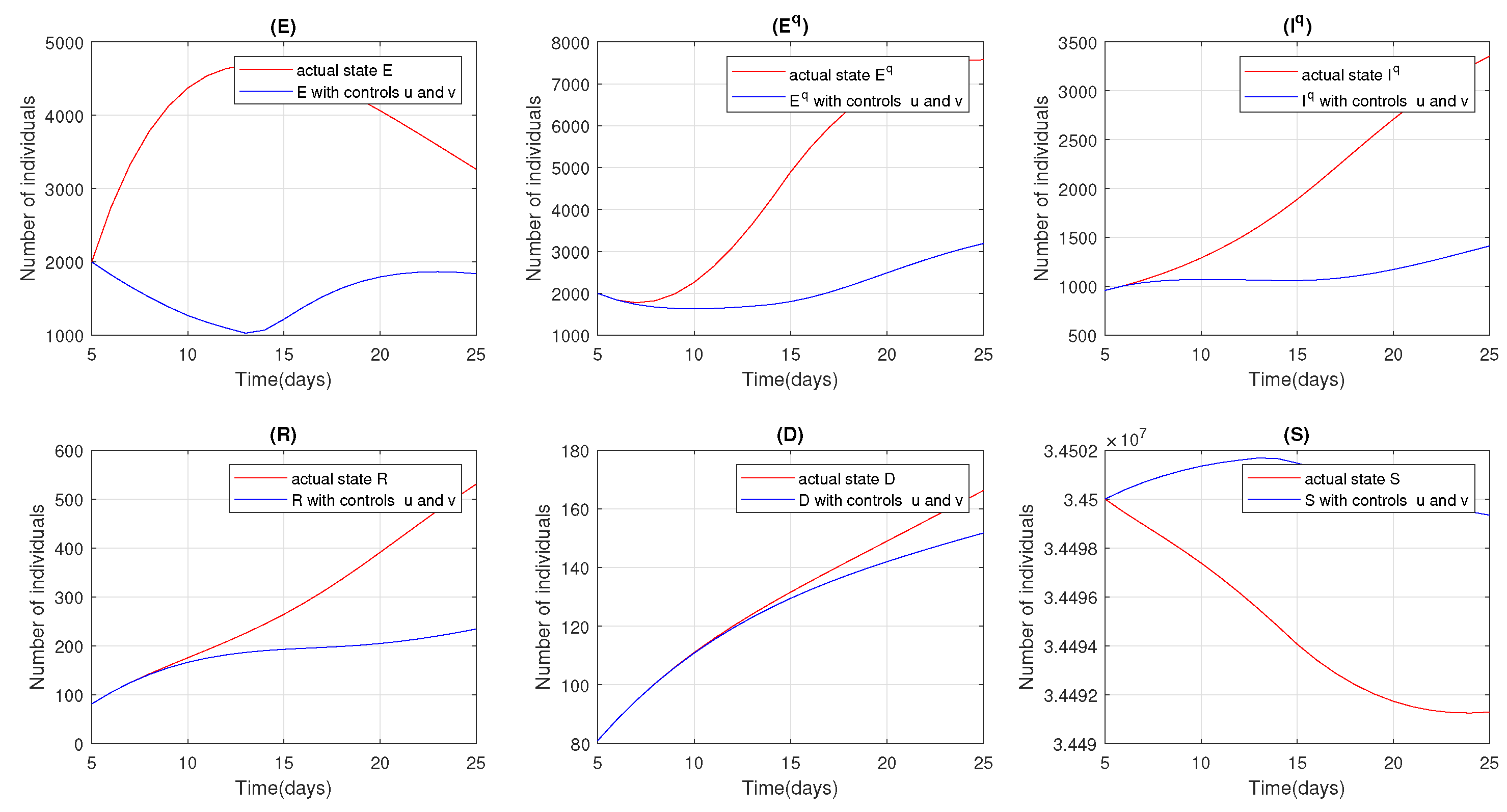
Figure 6 represents the dynamic evolution of the different states of the System (1) and a comparison with the states by introducing the optimal controls u and v during the period of 6 April to 25 April 2020.

From the evolution of the variables of the model, between the 6th and 26th April, with and without controls in Figure 6, we observe, clearly, the possibility of the impact of enhancing the efficacy of the lockdown in the epidemic situation of COVID-19 in Morocco. In fact, with an initial state $E_0=2000$ estimated on 6 April, we note an increasing evolution of the number of people exposed, which reaches a peak of 4800 people on 15 April, then decreases to 3200 cases on 26 April. On the other hand, by introducing optimal controls, i.e., the optimal containment strategy which reduces contact between people with the disease and susceptible people, we observe that the number of people exposed decreased to reach a minimum value on 15 April, then rebounded and grew to reach 1900 cases on 26 April.

The number of contacts $E_q$ decreases from $E_0^q=2000$ to reach 1800 cases on 8 April, then increases exponentially to reach its maximum value of 7650 at the end of the period. By introducing the optimal controls u and v, the number of contacts $E^q$ decreases at the start from 2000 to 1600 after 5 days and then increases to reach 3200 in 25 April.

For ($I^q$) the number of infected increased from 1000 cases in the beginning to 3400. On the other hand, by applying optimal containment, the number of infected remained constant in the beginning of 6 April to 13 April, then increased slightly to reach 1400 by the end of the year.

The estimated number of recovered, R, with and without control, initially increases in the same, However, with control it reaches 220 cases on 25 April and the number for the non-control group exponentially to reach 540 cases.

The estimated number of cases recovered, R, with and without control, initially increases in the same way, however, with control it reaches 220 cases in 25 April while this number, without control, grows exponentially up to 540.

Similarly, the number of deaths increases for both cases; we observe that they are the same between the period from 6 April to 13 April. In fact, the control strategy does not much affect the number of deaths as, with the optimal control, it reached 150 cases of death towards the end of the period and 168 for the cases without control.

The optimal control strategy reduces the susceptibility of the population by 11,500 by 25 April. However, without control, the number would increase by 447,100 persons.

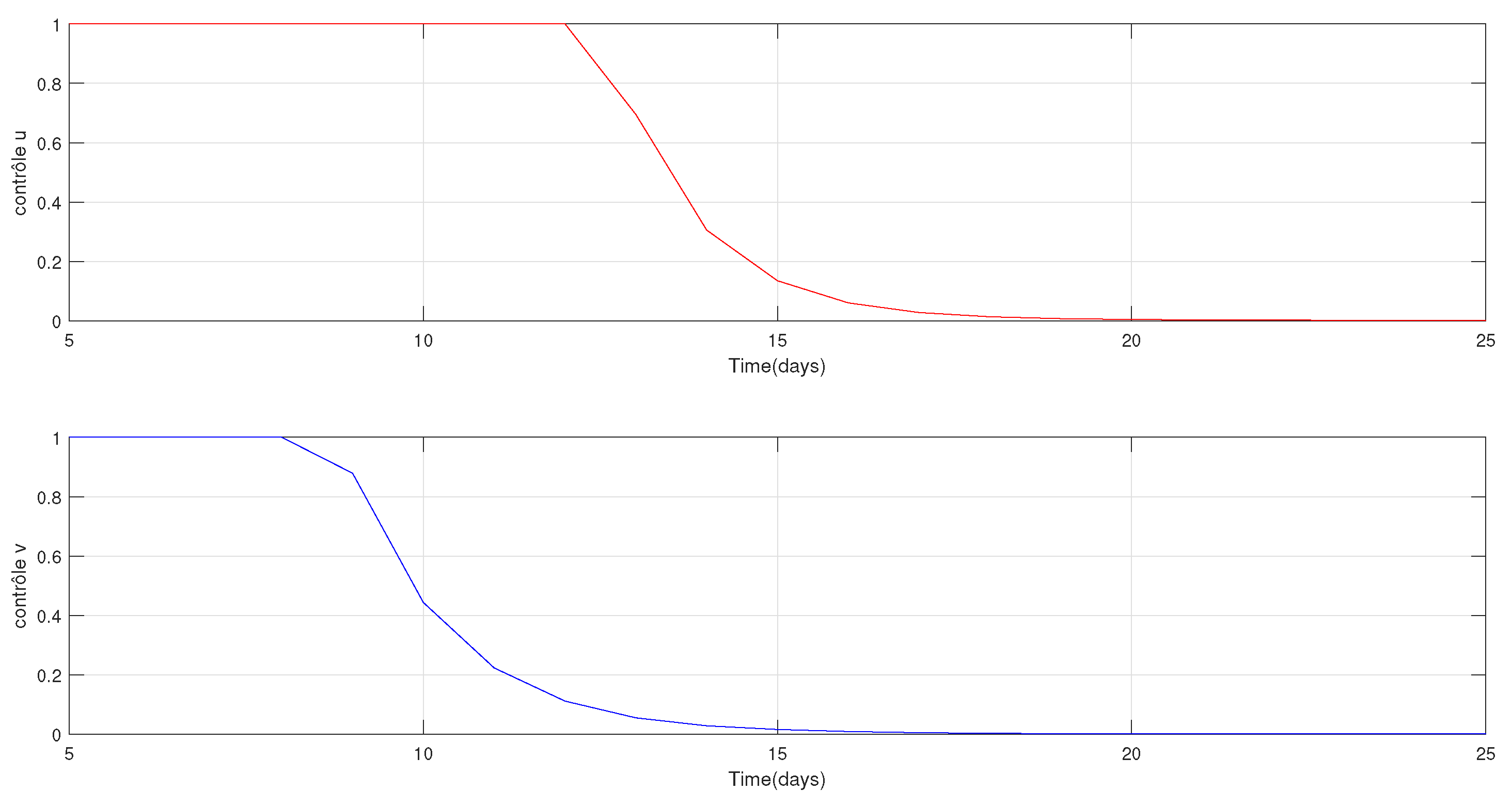
Note that the optimal control pair $(u,v)$, as shown in Figure 7, should be initiated for the exposed population (on the day 8) before the infected population (on the day $12)$.

3.2. Treatment Only

Figure 8 represents the dynamic evolution of the states of the system (1) with only the treatment and without lockdown. We remark that the treatment only does not affect much the populations of exposed E and $E^q$, as well as death D (with reduction of number of death by about 25 death) and susceptible S. However, it reduces the number infected in quarantine and increases the number of recovered. In fact, with the treatment, the number infected in quarantine cases would be reduced by 2050 cases and the number of recovered would be increased by about 700 cases.

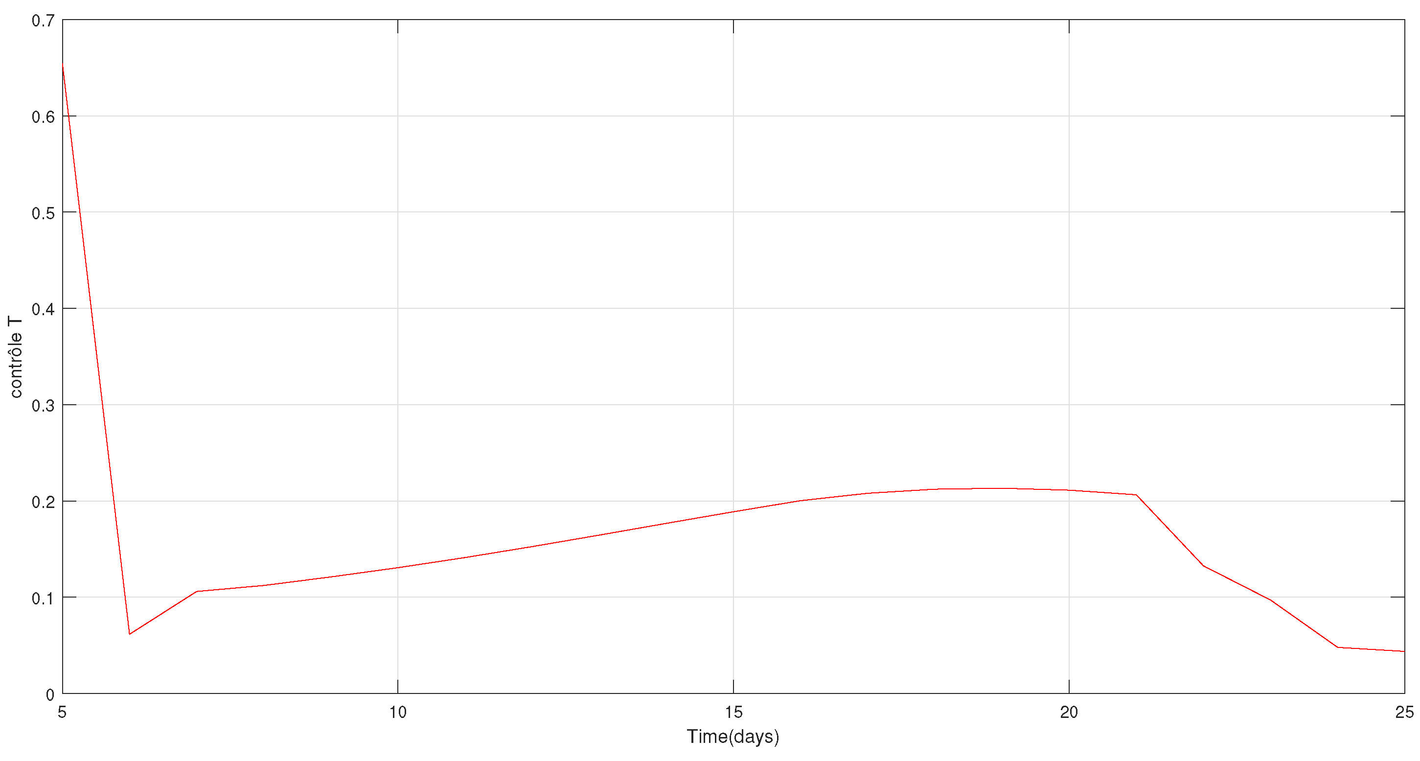
We note also that the optimal rate of cure is less, $22\%$, in most of the period between the 6th and 26th April, as shown in Figure 9.

3.3. Treatment and Lockdown Strategies

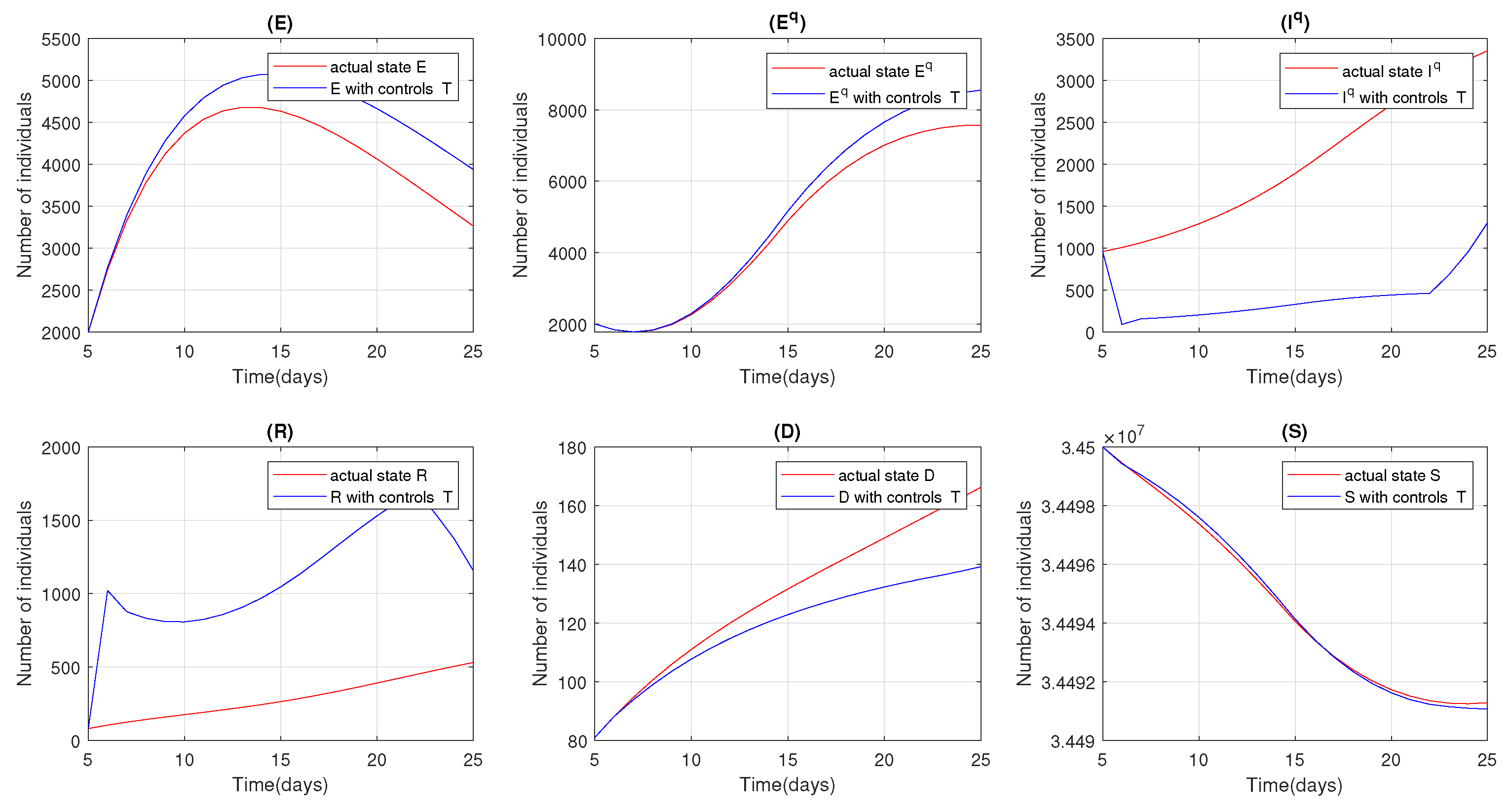
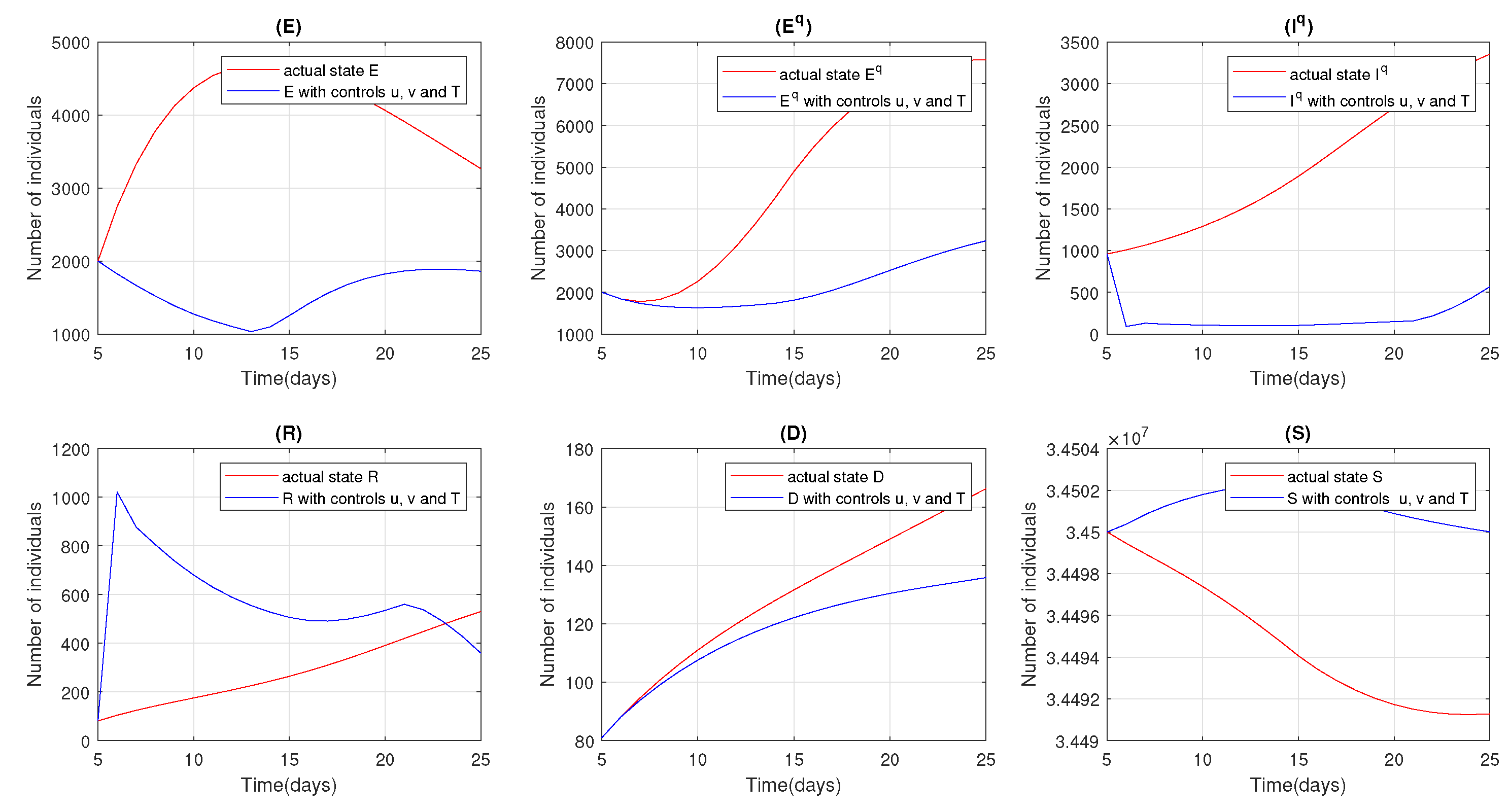
Now, we present the case where we combine the optimal treatment control and optimal lockdown strategy. From Figure 10, it can be seen that this pair of controls is more beneficial to contain COVID-19. In fact, we notice that for S, E and $E^q$, the outcome of applying these controls is similar to the case of lockdown only in Figure 6. However, there is a substantial reduction in the $I^q$, compared to the previous control approaches (treatment only and lockdown only). As for the number of deaths, we do not see much difference between combined control and treatment only. Although there is an increase in the number of recovered people in the beginning of studied period, surprisingly, we notice a slight reduction in this population compared to the fitted data.

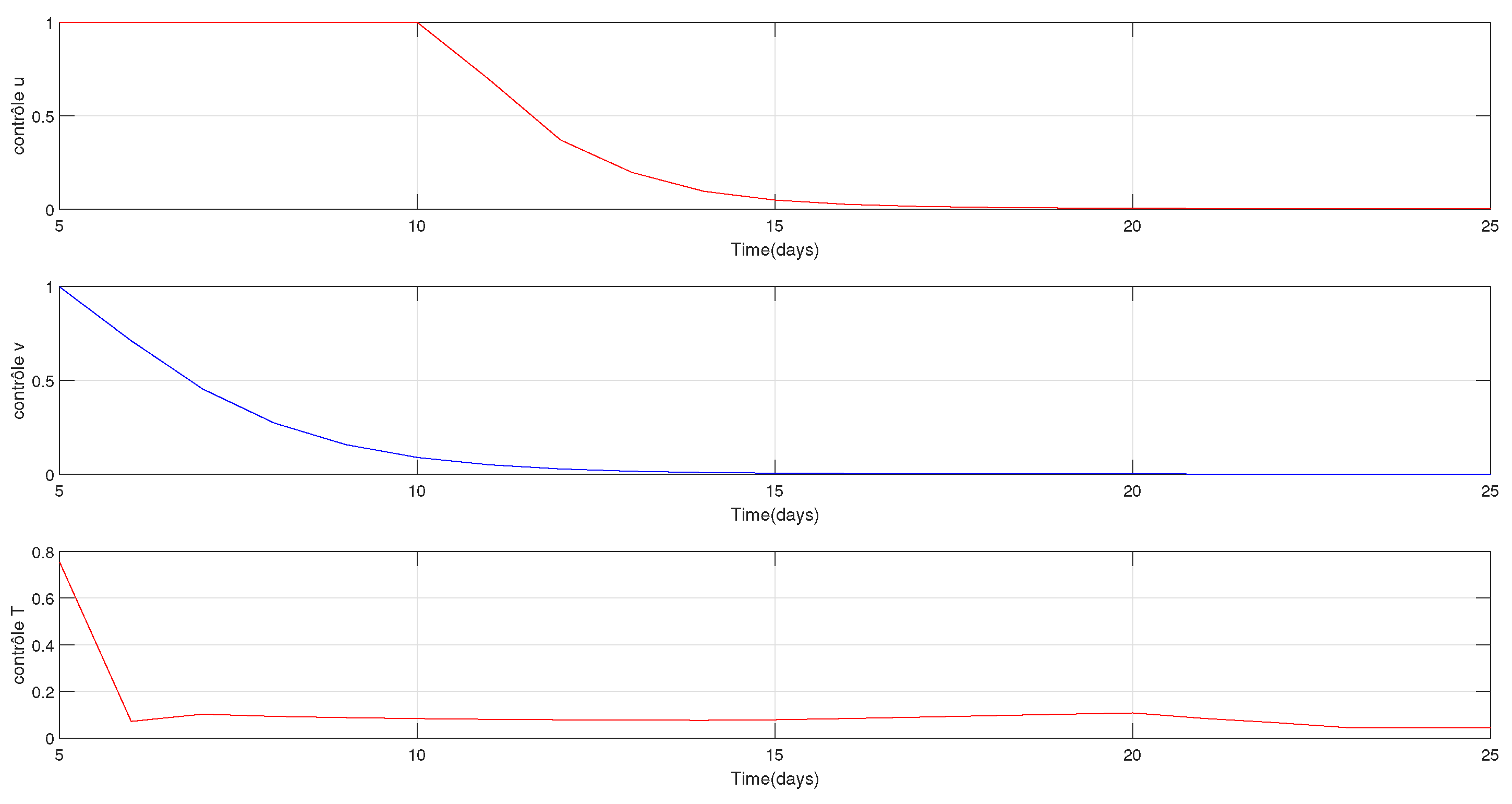
For the functions of optimal control strategy, we see clearly from Figure 11 that the optimal control pair $(u,v)$, should be initiated for the exposed population from 5 April and for the infected population from 10 April. The optimal treatment’s cure rate starts with $80\%$ and reaches less than $10\%$ over the rest of the period.

4. Conclusions

As the COVID-19 pandemic is still taking many lives around the globe ( over 766,000 death by 17 August 2020) and public health capacities are overwhelmed, many countries have rushed to take different control measures, such as lockdown, treatment, tracing contact and testing, that help to contain the spread of the disease. The question is what the best approach is to limit the impact of COVID-19 on the population. For this purpose, we studied the optimal strategy of lockdown during the COVID-19 in Morocco. First, using the nonlinear least-squares method, we fitted our discrete epidemic model to the COVID-19 data in the period between 6 April and 25 April 2020. By such a fitting, we determined the values of the parameters of our model. Next, we derived a control strategy for the COVID-19 that aims to minimize the exposed and infected populations and the treatment. We used optimal strategies to reduce the contact between the infected and the susceptible by adopting the quarantine strategy for the infectious and choosing containment throughout the country. Using the Pontryagin’s maximum principle, we obtained an explicit expression of the optimal control. Our numerical simulation of the optimal control showed the lockdown’s effect only, the treatment’s effect only, and both controls simultaneously. The lack of an anti-COVID-19 treatment or an effective vaccine against COVID-19, and limited medical resources are all factors that make it difficult to stop the transmission of this epidemic. For this reason, we have considered each control strategy separately. The first scenario is to use only closure, and this strategy gives a satisfactory health outcome, but, given that a nationwide lockdown has a major economic impact, it seems that we need another strategy to reduce its burden. Second, we looked at the scenario where only treatment was used. This control strategy also gives good results, especially for the number of infections, but it still appears insufficient when we see the number of people exposed. This control requires more medical equipment and more places available in hospitals. Finally, we combined the previous control strategies and found that this third control strategy is the best and most effective in terms of people isolated and the number of infections. Thus, we have alleviated the burden on medical establishments as well as the economic side effects of the lockdown.

References

- Huang, C.; Wang, Y.; Li, X.; Ren, L.; Zhao, J.; Hu, Y.; Zhang, L.; Fan, G.; Xu, J.; Gu, X.; et al. Clinical features of patients infected with 2019 novel coronavirus in Wuhan, China. Lancet 2020, 395, 497–506. [Google Scholar] [CrossRef] [Green Version]
- Sirkeci, I.; Yucesahin, M.M. Coronavirus and Migration: Analysis of Human Mobility and the Spread of COVID-19. Migr. Lett. 2020, 17, 379–398. [Google Scholar] [CrossRef] [Green Version]
- WHO. Coronavirus Disease (COVID-19) Pandemic. 2020. Available online: https://www.who.int/emergencies/diseases/novel-coronavirus-2019 (accessed on 10 August 2020).
- Cao, Z.; Zhang, Q.; Lu, X.; Pfeiffer, D.; Wang, L.; Song, H.; Pei, T.; Jia, Z.; Zeng, D.D. Incorporating human movement data to improve epidemiological estimates for 2019-nCoV. medRxiv 2020. [Google Scholar]
- Chen, T.M.; Rui, J.; Wang, Q.P.; Zhao, Z.Y.; Cui, J.A.; Yin, L. A mathematical model for simulating the phase-based transmissibility of a novel coronavirus. Infect. Dis. Poverty 2020, 9, 1–8. [Google Scholar] [CrossRef] [PubMed] [Green Version]
- Qianying, L. A conceptual model for the coronavirus disease 2019 (COVID-19) outbreak in Wuhan China with individual reaction and governmental action. Int. J. Infect. Dis. 2020, 93, 211–216. [Google Scholar]
- Liu, X.; Hewings, G.J.; Qin, M.; Xiang, X.; Zheng, S.; Li, X.; Wang, S. Modelling the Situation of COVID-19 and Effects of Different Containment Strategies in China with Dynamic Differential Equations and Parameters Estimation. medRexiv 2020. SSRN 3551359. [Google Scholar] [CrossRef]
- Rabajante, J.F. Insights from early mathematical models of 2019-nCoV acute respiratory disease (COVID-19) dynamics. arXiv 2020, arXiv:2002.05296. [Google Scholar]
- You, C.; Deng, Y.; Hu, W.; Sun, J.; Lin, Q.; Zhou, F.; Pang, C.H.; Zhang, Y.; Chen, Z.; Zhou, X.H. Estimation of the time-varying reproduction number of COVID-19 outbreak in China. Int. J. Hyg. Environ. Health 2020, 228, 113555. [Google Scholar] [CrossRef] [PubMed]
- Zhao, S.; Lin, Q.; Ran, J.; Musa, S.S.; Yang, G.; Wang, W.; Lou, Y.; Gao, D.; Yang, L.; He, D.; et al. Preliminary estimation of the basic reproduction number of novel coronavirus (2019-nCoV) in China, from 2019 to 2020: A data-driven analysis in the early phase of the outbreak. Int. J. Infect. Dis. 2020, 92, 214–217. [Google Scholar] [CrossRef] [PubMed] [Green Version]
- Zakary, O.; Bidah, S.; Rachik, M. The Impact of Staying at Home on Controlling the Spread of COVID-19: Strategy of Control. Mex. J. Biomed. Eng. 2020, 42, 10–26. [Google Scholar]
- HCP. High Commission for Planning of Morocco, Les taux (en p mille) de natalite, de migration, d’accroissement naturel et global pour la population du Maroc, 2010–2050. Available online: https://www.hcp.ma/Les-taux-en-p-mille-de-natalite-de-migration-d-accroissement-naturel-et-global-pour-la-population-du-Maroc-2010-2050_a685.html (accessed on 5 July 2020).
- Dabbs, K. Optimal Control in Discrete Pest Control Models, University of Tennessee Honors. Ph.D. Thesis, University of Tennessee, Knoxville, TN, USA, 2010. [Google Scholar]
- Boltyanskiy, V.; Gamkrelidze, R.V.; Mishchenko, Y.; Pontryagin, L. Mathematical Theory of Optimal Processes; Wiley: New York, NY, USA, 1962. [Google Scholar]
- Lenhart, S.; Workman, J.T. Optimal Control Applied to Biological Models; CRC Press: Boca Raton, FL, USA, 2007. [Google Scholar]
Figure 1.
The flowchart of the model (1).
Figure 2.
Real data of Morocco, from 6 April to 25 April. (a) Active infected cases, (b) Recovered individuals and (c) dead individuals.
Figure 3.
The data fitting of I in (a), R in (b) and D in (c) to estimate the parameters of the model.
Figure 4.
Residuals of the (a) active infected cases, (b) recovered individuals and (c) dead individuals.
Figure 5.
Normality test for the (a) active infected cases, (b) recovered individuals and (c) dead individuals.
Figure 6.
Evolutionary dynamics of the model with optimal controls u and v.
Figure 7.
The optimal control functions u and v.
Figure 8.
Evolutionary dynamics of SEIRQD model with optimal control T.
Figure 9.
The optimal control function T.
Figure 10.
Evolutionary dynamics of SEIRQD model with optimal controls u, v and T.
Figure 11.
The optimal control function u, v and T.