A Bimodal Lognormal Distribution Model for the Prediction of COVID-19 Deaths


Department of Civil and Industrial Engineering, University of Pisa, Largo Lucio Lazzarino, I-56122 Pisa, Italy
Appl. Sci. 2020, 10(23), 8500; https://doi.org/10.3390/app10238500
Submission received: 28 October 2020
/
Revised: 23 November 2020
/
Accepted: 26 November 2020
/
Published: 28 November 2020
(This article belongs to the Special Issue Spreading of Infection Diseases like COVID-19 and Influenza: Modelling and Propagation Control)
Abstract
:The paper presents a phenomenological epidemiological model for the description and prediction of the time trends of COVID-19 deaths worldwide. A bimodal distribution function—defined as the mixture of two lognormal distributions—is assumed to model the time distribution of deaths in a country. The asymmetric lognormal distribution enables better data fitting with respect to symmetric distribution functions. Besides, the presence of a second mode allows the model to also describe second waves of the epidemic. For each country, the model has six parameters, which are determined by fitting the available data through a nonlinear least-squares procedure. The fitted curves can then be extrapolated to predict the future trends of the total and daily number of deaths. Results for the six continents and the World are obtained by summing those computed for the 210 countries in the Our World in Data (OWID) dataset. To assess the accuracy of predictions, a validation study is first conducted. Then, based on data available as of 30 September 2020, the future trends are extrapolated until the end of year 2020.
1. Introduction
For over a century, the use of mathematical models has been introduced to describe and predict the course of epidemics [1]. Following the first pioneering studies, epidemiologic models of growing complexity have been developed [2].
Models may be classified as either based on transmission dynamics or phenomenological. Transmission dynamics models aim at describing the physical, biological, and societal mechanisms underlying the outbreak and spread of a disease. On the one hand, they can be very helpful in understanding the behaviour of epidemics and the effects of human interventions. On the other hand, transmission dynamics models rely sometimes on a large number of parameters, which may be difficult to evaluate in practice with the necessary accuracy [3]. As an alternative, phenomenological models can be used. These are based on a limited number of parameters that can be calibrated through fitting of the available data. Phenomenological models do not aim at understanding the mechanisms underlying an epidemic, but can be used for efficient and rapid forecasts [4]. For instance, Pell et al. used phenomenological models to forecast the evolution of the 2015 Ebola epidemic [5].
Both transmission dynamics models and phenomenological models were used to describe the 2020 COVID-19 pandemic caused by the SARS-CoV-2 coronavirus [6]. Among the former, the classic susceptible-infected-recovered (SIR) model and modifications thereof have been widely used. Among the latter, models based on either the logistic or Gaussian distribution functions have been proposed. Batista applied both the SIR and logistic models to predict the final size of the COVID-19 epidemic in China. By processing data available up to 20 February 2020, he estimated a total number of cases at the end of the epidemic equal to approximately 84,500 from the SIR model and 83,700 from the logistic model [7]. Retrospectively, such predictions turned out to be very accurate if compared to the official number of cases reported four months later. As of 20 June 2020, the official number of cases in China was 84,524. Mackolil and Mahanthesh used the SIR and logistic models to describe the COVID-19 outbreak India. They processed the official data available from 9 March to 9 May 2020 for three states (Karnataka, Kerala, and Maharashtra), characterised by a significant spread of the epidemic. For the most affected state, Maharashtra, the SIR model estimated the final number of cases at 46,678, whereas the logistic model predicted 43,993 cases [8]. Retrospectively, such predictions turned out to be dramatically underestimated. One month later, as of 9 June 2020, 90,787 cases were reported. As of early August 2020, more than 500,000 cases were registered [9]. Paggi used particle swarm optimisation to identify the parameters of a SIR model of the COVID-19 outbreak in Italy. He focused on the four most affected regions (Lombardy, Emilia Romagna, Valle d’Aosta, and Veneto). The machine learning approach was found to be robust for the identification of a large set of model parameters. The model results showed that lockdown measures had a major impact especially in Lombardy [10]. Martelloni and Martelloni used the logistic model to analyse the evolution of the COVID-19 epidemic in Italy. They processed data available up to 1 April 2020 and forecast about 138,500 cases and 19,900 deaths by the end of the epidemic [11]. Retrospectively, such figures turned out to be quite underestimated. One month later, as of 1 May 2020, official statistics reported 205,463 cases and 27,967 deaths with the epidemic still spreading in Italy. Schlickeiser and Schlickeiser used a Gaussian model to predict the development of the COVID-19 epidemic in Germany. Based on the data available as of 30 March 2020, they predicted the peak of the death rate to occur on 18 April 2020 + (−3.4, +5.4) days. Their prediction turned out to be in excellent agreement with the actual peak registered on 16 April 2020 [12]. Schüttler et al. discussed about the choice of asymmetric functions to model the COVID-19 death rate, but eventually decided in favour of the simplest symmetric, bell-shaped Gaussian function. Based on data available as of 2 April 2020, they predicted the final number of deaths for 25 countries. In a note added in proof, the authors compare their theoretical predictions with the data available as of 2 June 2020. Good agreement is obtained for some countries, such as France and Germany. Instead, the model appears to underestimate the real data of some other countries, such as Italy and Spain [13]. Interestingly, less accurate predictions are obtained for countries, where the actual time distribution of deaths presents a higher degree of asymmetry.
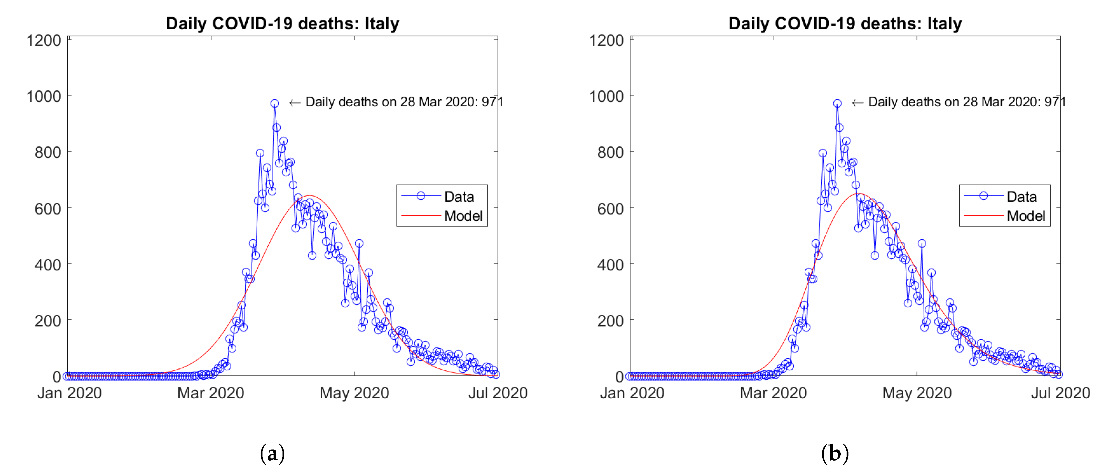
As a matter of fact, upon inspection of the available data, the number of infections or deaths in a given country (or geographical region) does not follow in general a symmetric distribution in time. Rather, after reaching the peak value, a descending branch less steeper than the ascending one can be often observed. In such cases, a better fit of the real data can be obtained by using asymmetric distribution functions—such as, for instance, the lognormal distribution—instead of the symmetric logistic and Gaussian functions. As an example, Figure 1 shows the daily number of COVID-19 deaths reported in Italy in the first semester of year 2020. Data have been fitted by using both a Gaussian distribution function (Figure 1a) and a lognormal distribution function (Figure 1b). The residual norms computed in the two cases were 202,818,961 and 63,831,005, respectively. Application of the same distribution functions to fit the data of all of the 210 countries in the Our World in Data (OWID) dataset [14] for the same period furnished cumulative residual norms equal to 3,467,666,524 and 1,365,052,591, respectively. Such results prove, beyond the qualitative comparison between the curves, the superiority of the lognormal distribution function to fit the data of the present problem.
In a preliminary analysis of the Italian epidemic, the author used a lognormal distribution function to fit the number of deaths per day reported in each Italian administrative region. By processing the data available as of 2 May 2020, the total forecast number of deaths in Italy at the end of the first wave of the epidemic was 35,261 [15]. As of 31 August 2020, the official data reported 35,477 deaths with an error of less than 1% [16].
When looking at the time evolutions of the number of COVID-19 cases and deaths around the world, different trends are observed for each country and geographic region. As of September 2020, China and many European countries have overcome the first wave of the epidemic. Other countries—such as, for instance, Australia, Israel, Japan, Romania, and the United States—are being hit by second waves of the epidemic. In Iran, a third wave of the epidemic is going on. Such new waves appear as second (or third) peaks in the time distributions of infections and deaths. In some cases, e.g., the United States, the second waves could be the result of first waves affecting different internal states or regions. Anyway, a better data fitting for such countries requires the adoption of suitable bimodal (or multimodal) distribution functions. Any theoretical model aimed at describing the pandemic at the global level should account for the variability in both space and time of the monitored trends (cases, hospitalisations, recoveries, fatalities, etc.).
The aim of the present work is to develop a phenomenological epidemiological model for the description of the worldwide trends of COVID-19 deaths and their prediction in the short-to-medium (1 and 3 months, respectively) term in a business-as-usual scenario. The model assumes a bimodal lognormal distribution in time of the deaths per country. A nonlinear least squares procedure is used to fit the available data and determine the six model parameters for each country. Then, the obtained curves are extrapolated to forecast the future trends. Results for the six continents and the World are obtained by summing those computed for the belonging countries.
The paper is organised as follows. In Section 2, details are given about the used dataset. Section 3 presents the mathematical model and its numerical implementation. In Section 4, a validation study of the model is illustrated. Section 5 presents the results obtained for the main countries, as well as the forecasts for the six continents and the whole World. Discussion follows in Section 6. In Section 7, some conclusive comments and indications for future developments are given. Appendix A presents a comparison of the model predictions with actual data, which became available after the submission of the manuscript.
2. Data
Data used in the present study are obtained from the Our World in Data (OWID) COVID-19 dataset [14]. The OWID dataset is based on official data published by the European Center for Disease Prevention and Control (ECDC). The ECDC publishes daily statistics on the COVID-19 pandemic by collecting and harmonising data from the national health agencies around the world [17].
The OWID dataset is updated daily and includes data on country population, confirmed cases, deaths, testing, etc. starting from 31 December 2019. The dataset is subdivided into 211 locations: 210 countries and an international cluster (reporting the cases from an international conveyance in Japan), besides a World summary. For the present purposes, for each location and date, the daily (new) and total (cumulative) number of deaths are extracted and considered for further elaboration.
3. Methods
3.1. Mathematical Model
The daily number of deaths in a country is assumed to be distributed in time according to a bimodal lognormal distribution, here defined as the mixture of two lognormal distributions [18]:
where t represents time, A is an amplitude factor, is the mixing parameter, and respectively are the mean value and standard deviation of the natural logarithm of t for the first lognormal distribution, and are the same quantities for the second lognormal distribution.
The total number of deaths is given by the integral in time of :
where denotes the error function. As , the function tends asymptotically to the amplitude, A, which can be interpreted as the total number of deaths expected at infinite time.
3.2. Numerical Implementation
A nonlinear least-squares procedure is used to fit the available data and determine the model parameters. The fitting procedure is implemented into a MATLAB script called COVID19_BiLog_World.m, available in the Supplementary Materials.
The OWID COVID-19 dataset is downloaded as a CSV file named owid-covid-data.csv. For each location in the dataset, the daily number of deaths, , and total number of deaths, , are extracted. Here, the time variable, t, is expressed in days. It runs from 1 (first day of dataset: 31 December 2019) to (last day of simulations: 31 December 2020). The user can choose the days corresponding to the end of the fitting range, , and the end of the extrapolation interval, .
For each location, the procedure determines the days, and , at which attains its first and second maxima. Then, the function representing the theoretical total number of deaths, , is fitted against the reported total number of deaths, , in the range between and . The procedure uses the MATLAB lsqcurvefit function, which requires a minimum value, a guess value, and a maximum value for each parameter [19]. These are specified as detailed in Table 1.
As a result, the following six parameters are determined for each country: A, , , , , and . Here, and respectively denote the mode and standard deviation of the first lognormal distribution. Likewise, and are the same quantities for the second distribution [18]. The obtained parameters are substituted into Equations (1) and (2). Thus, the theoretical estimates of the daily and total number of deaths are computed between and . The procedure is repeated for each of the 211 locations. Hence, the predicted time trends for the six continents and the World are obtained by summing those computed for the belonging countries.
The MATLAB script saves the results obtained for each location—in terms of fitted parameters, residual norm and exit flag returned by the lsqcurvefit function, actual number of deaths (at ), and forecast number of deaths (at )—into a CSV file called COVID19_BiLog_World.csv. Besides, for each (selected) country, continent, and the World, two plots are created and saved in PNG format: (i) the daily number of deaths and (ii) the total number of deaths, as functions of time.
4. Validation
4.1. Correlation Study
To assess the correlation between the model predictions and actual data, a first validation study has been carried out by using data available up to 30 June 2020. From this date, extrapolations have been conducted to forecast the total number of deaths as of 15 and 31 July, 15 and 31 August, 15 and 30 September 2020.
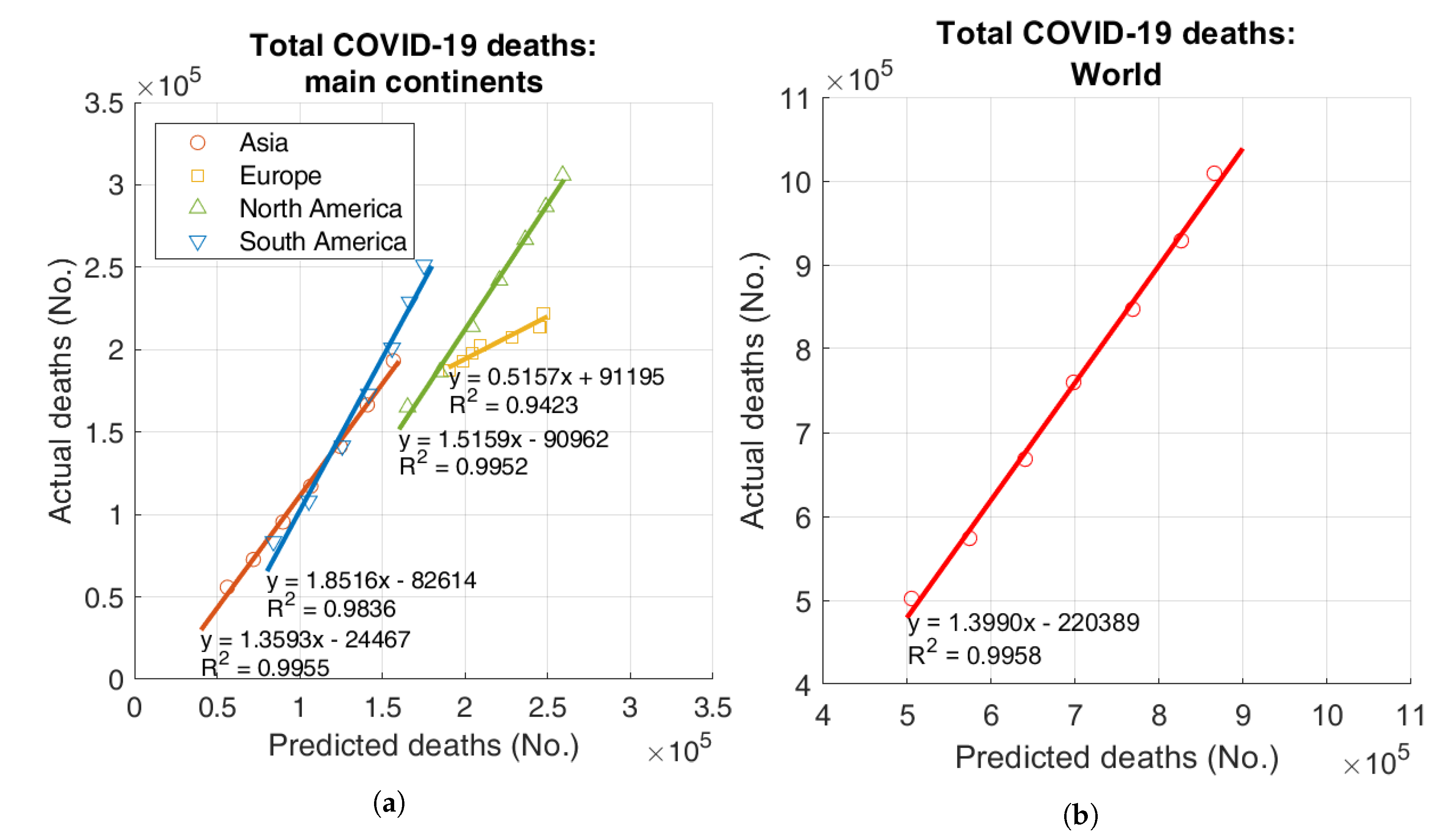
Figure 2 shows scatter plots of the actual vs. predicted number of deaths for the main continents and the World. Regression lines with the values of intercept, slope, and coefficient of determination are also shown. Asia, North and South America have slopes larger than 1, thus highlighting a tendency of the model to underestimate the actual data; instead, Europe has a slope less than 1, corresponding to a tendency to overestimation (Figure 2a). For the whole World, the slope is , thus highlighting a general tendency of the model to underestimate data (Figure 2b). The coefficient of determination for the World is .
4.2. Retrospective Predictions
To use a larger dataset to assess the accuracy of the model predictions, a second validation study has been carried out. In this case, the model has been used to predict retrospectively the (known) number of deaths as of September 2020. Different dates were chosen for the end of the fitting range: from 30 June to 15 September 2020. Table 2 shows the actual and forecast number of deaths in the six continents and the World. Percentages in parentheses represent the errors of the theoretical predictions with respect to the actual data, calculated as .
The largest percent errors are observed for Oceania. In particular, the three-month forecasts (as of 30 June and 15 July 2020) are largely in defect because they do not take into account the effects of the second wave occurred in this continent since the end of July 2020. Oceania, however, carries a marginal weight in the global balance. Relatively large errors can be noted also in the three-month predictions for South America, Africa, and Asia. Actually, such predictions are computed on a relatively little amount of data, which causes poor quality of data fitting and extrapolation (as of June 2020, the epidemic was still at an early stage in many countries of these three continents). Three-month forecasts for North America and Europe are the most accurate, thanks to the large amount of data fitted (as of June 2020, the first peaks of the epidemic were already overcome). Two-month predictions (as of 31 July and 15 August 2020) and one-month predictions (as of 31 August and 15 September 2020) show absolute errors less than about 15% and 10%, respectively, for all of the continents (apart from Oceania).
Interestingly, in the World summary, plus and minus errors seem to compensate and a much more stable trend of predictions is observed. The three-, two-, and one-month forecasts are affected by errors less than about 20%, 10%, and 1%, respectively.
Based on the above, it can be concluded that the model is capable of capturing future trends with reasonable accuracy. Larger errors are expected for countries and continents with little amount of fitted data and where the epidemic is still at an early stage. Predictions for single continents may be affected by larger errors with respect to the World summary.
4.3. Extrapolation Error
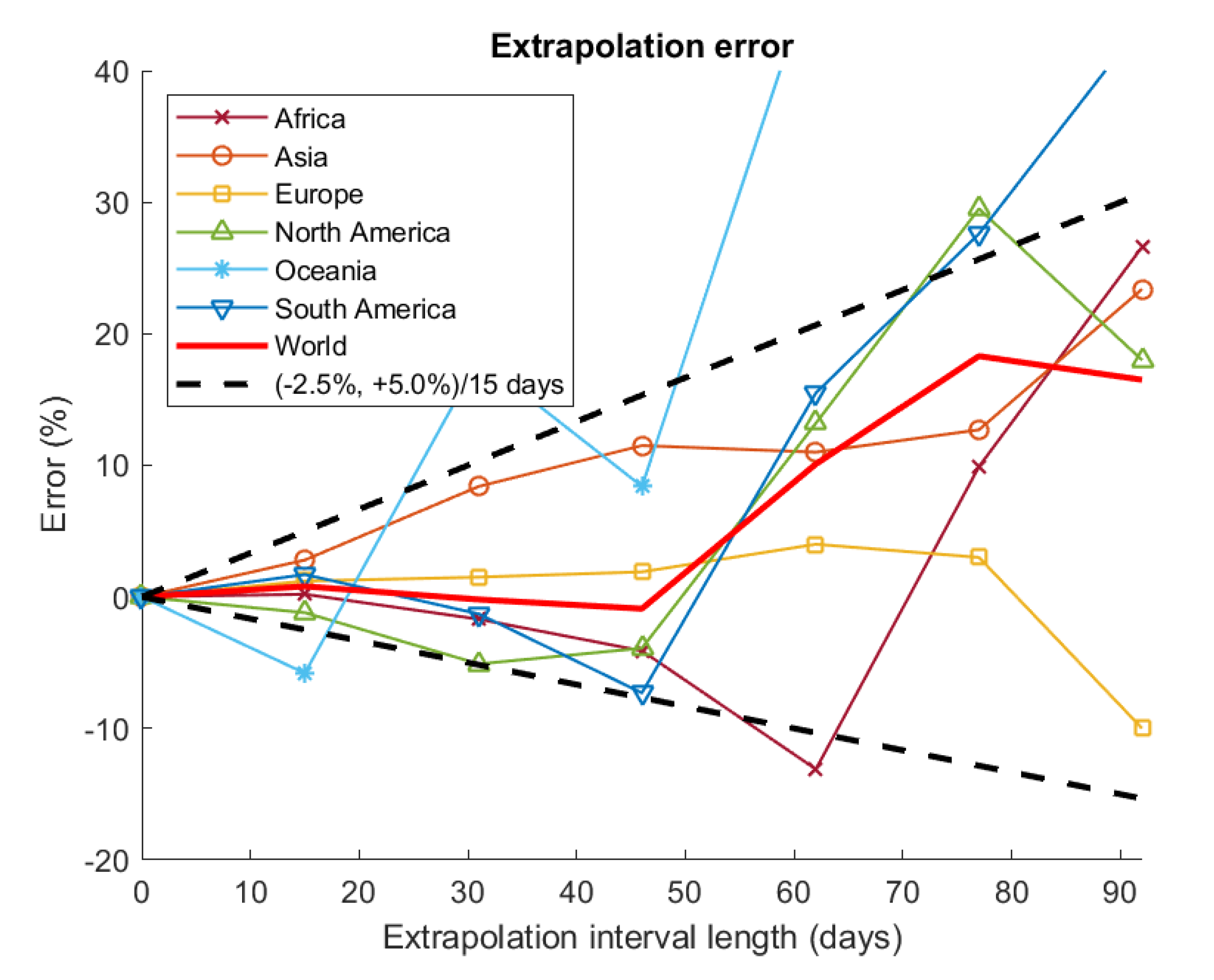
Figure 3 shows the extrapolation errors obtained in the retrospective predictions as functions of the extrapolation interval length, i.e., the number of days included between the end of the fitting range and the forecast date. For the main continents and the World, the extrapolation errors can be enveloped approximately by assuming a lower bound error rate of −2.5%/15 days and an upper bound error rate of +5.0%/15 days.
As concerns future predictions, similar error trends are expected for the extrapolation of the fitted curves. Extrapolation errors should increase with the length of the extrapolation intervals. Conversely, errors should decrease with an increase in the amount of fitted data. Hence, extrapolations from data known as of 30 September 2020 should be more accurate than the extrapolations carried out in the retrospective study. Anyway, to be on the safe side, the same error rates (−2.5%, +5.0%)/15 days will be assumed also to define confidence intervals for future predictions.
5. Results
Result presented in this section have been obtained by fitting the available data between 31 December 2019 and 30 September 2020. Then, extrapolations have been computed up to 31 December 2020.
Table 3 shows the results obtained for the two countries with the largest number of actual COVID-19 deaths in each continent. In the next subsections, plots are presented and commented for a few representative countries, as well as for the six continents and the World. The complete results and plots (for all of the 211 locations of the OWID dataset, as well as the continental and World summaries) are available in the Supplementary Materials.
5.1. Asia
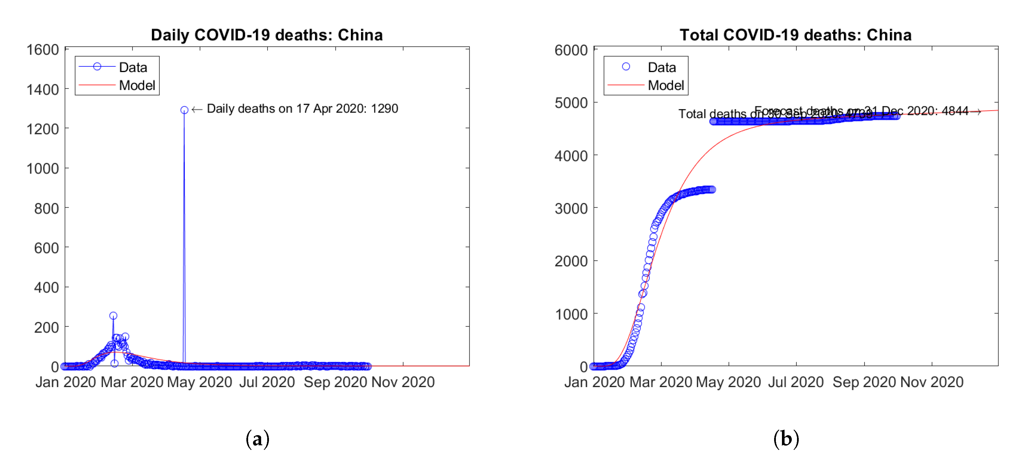
The first COVID-19 cases were reported in Wuhan, China in December 2019 [20]. Figure 4 shows the actual and predicted trends of COVID-19 deaths in this country. On 17 April 2020, the daily number of deaths (Figure 4a) presents an isolated peak of 1290 deaths due to a change in the tally criteria [21]. Correspondingly, a strong discontinuity can be observed in the total number of deaths (Figure 4b). The model does not fit exactly such an artificial discontinuity, but reproduces well the overall trend. In the last months, the official number of deaths shows only a very slight increase, thus indirectly demonstrating the effectiveness of the strict lockdown imposed by local Authorities.
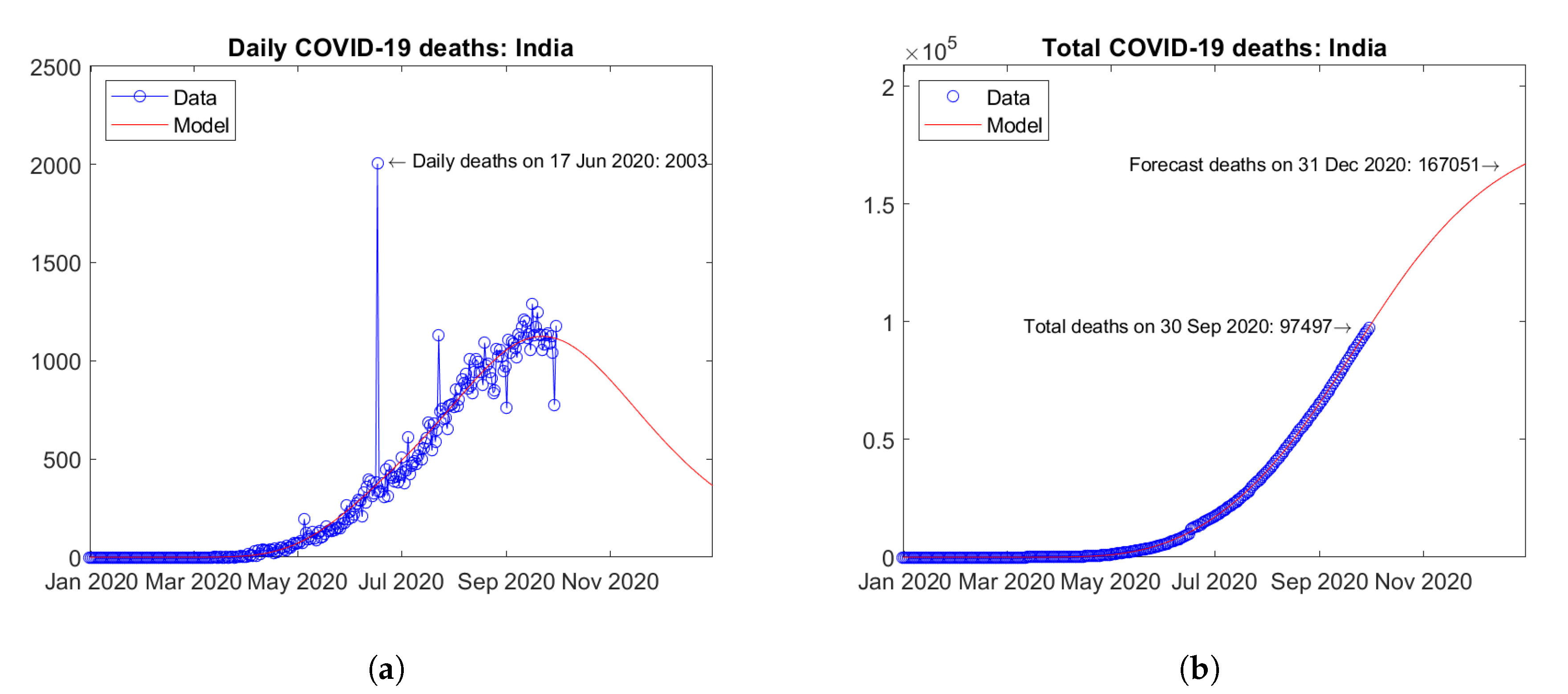
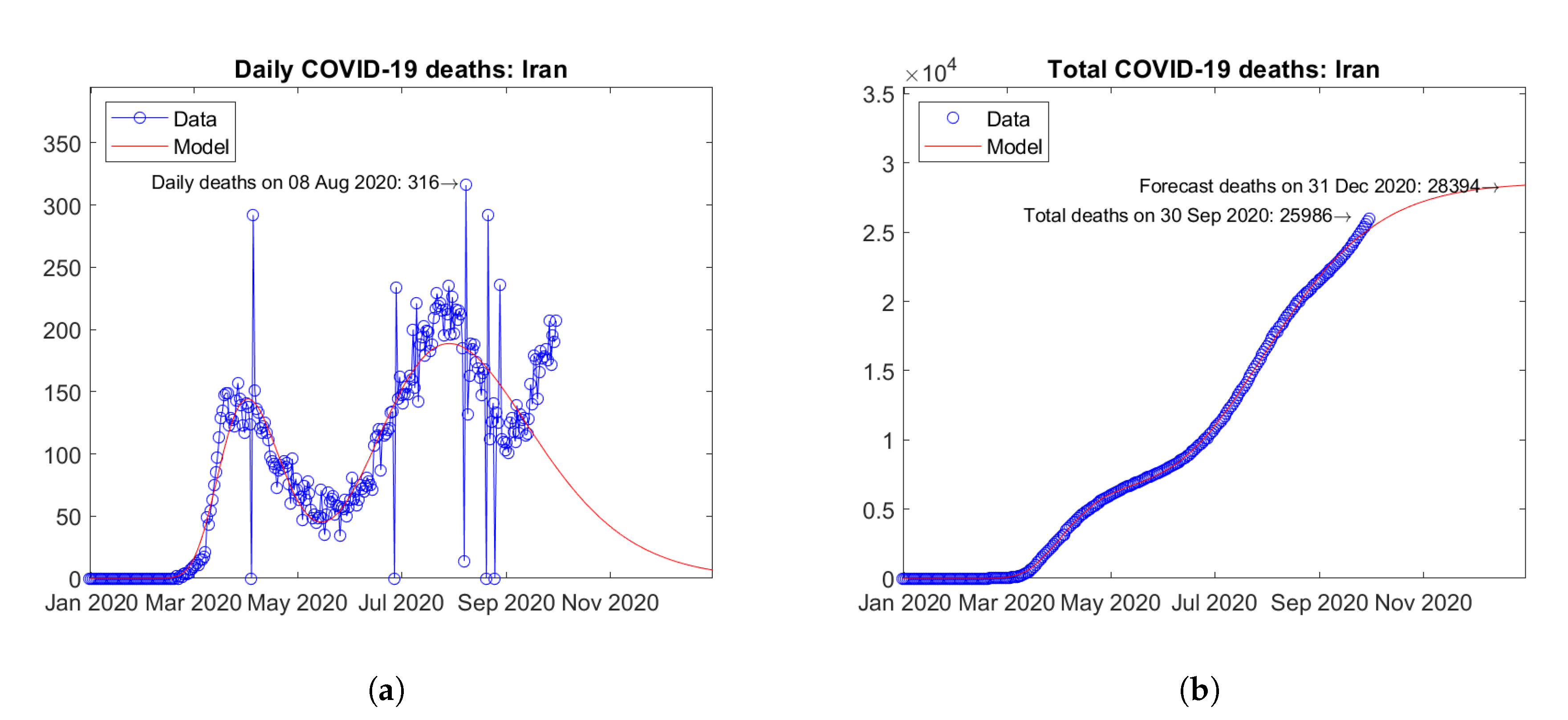
The two Asian countries with the largest number of actual and predicted COVID-19 deaths are India (Figure 5) and Iran (Figure 6). Quite different trends in time are observed in the two countries. In India, the daily deaths seem to have reached a peak value in September 2020 and a descending trend is expected afterwards (Figure 5a). The model is able to fit very well the available data, thus the extrapolation may be considered reliable (Figure 5b). In Iran, after a first wave of the epidemic with a peak of daily deaths in April 2020, a second wave has hit the country with a higher peak of daily deaths in August 2020. Recent data show the onset of a third wave with a tendency towards an even higher third peak (Figure 6a). The model assumes at most two peaks, so it is not able to fit very well all of the available data. Based on the above, the prediction of the total number of deaths at the end of 2020 may turn out to be underestimated for this country (Figure 6b).
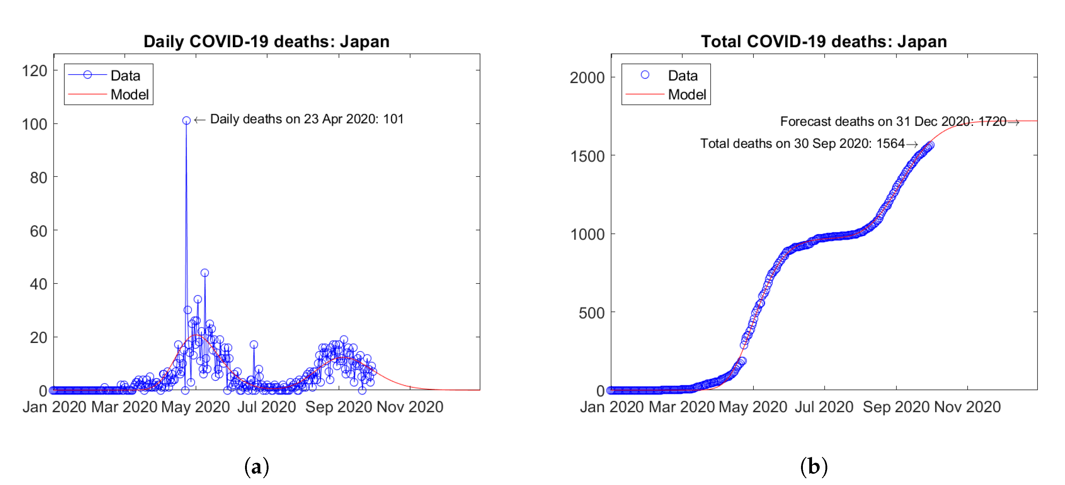
Israel (Figure 7) and Japan (Figure 8) are considered to be representative countries hit by second waves of the epidemic. In Israel, a first peak of daily deaths was observed in April 2020 and a second peak is expected in October 2020 (Figure 7a). In Japan, after a first peak of daily deaths in May 2020, a second peak was reached in September 2020 (Figure 8a). In both cases, the assumed bimodal distribution function enables very good fitting of data (Figure 7b and Figure 8b).
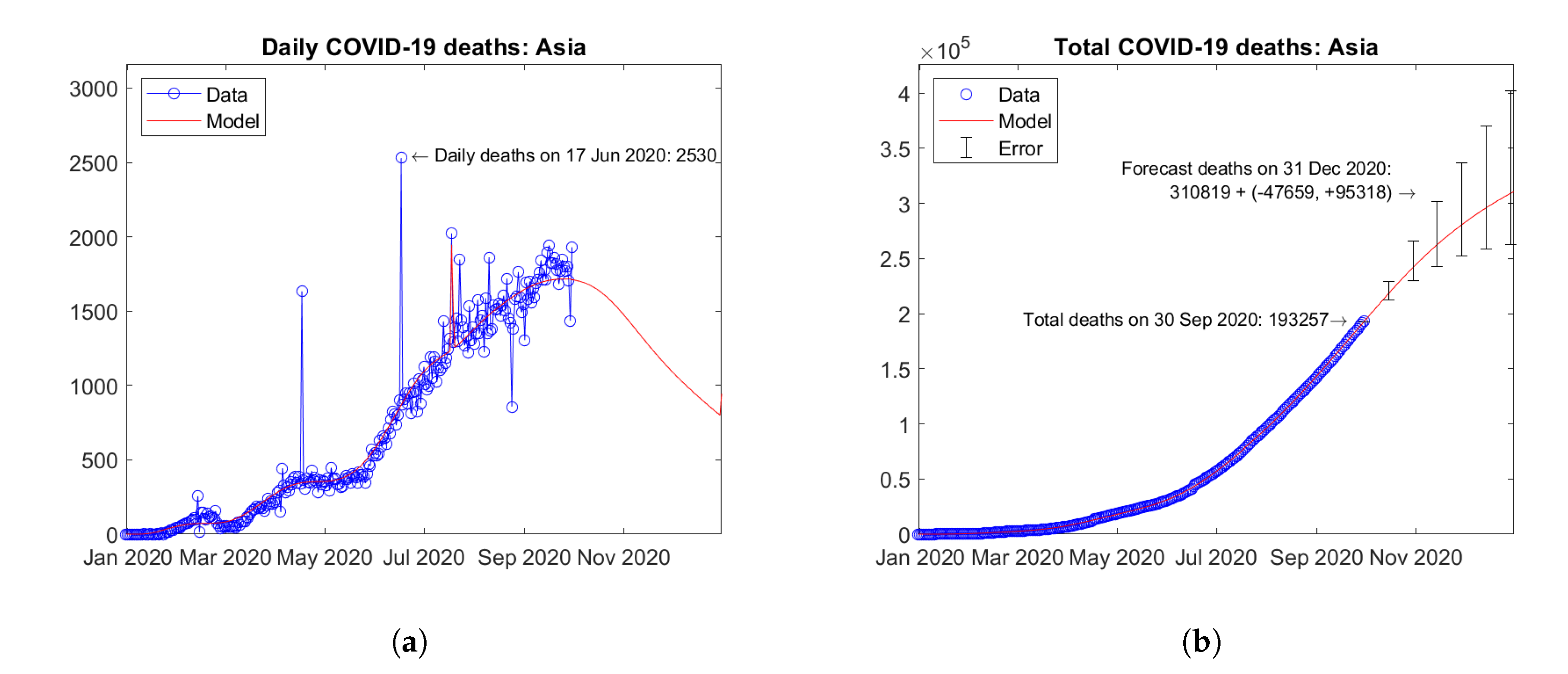
Figure 9 shows the time trends obtained for the Asiatic continent by summing the available data and model predictions for each country. Several peaks of daily deaths can be observed, as a result of the different local trends (Figure 9a). Overall, the current trend is descending and a weakening of the epidemic in the continent is expected by the end of year 2020. Figure 9b shows the total number of deaths in the continent with an extrapolation of the model until the end of year 2020. The predicted trend is strongly increasing. Error bars correspond to the error rate (−2.5%, +5%)/15 days estimated through the validation study. The forecast total number of COVID-19 deaths on 31 December 2020 in Asia is 310,819 + (−47,659, +95,318).
5.2. Europe
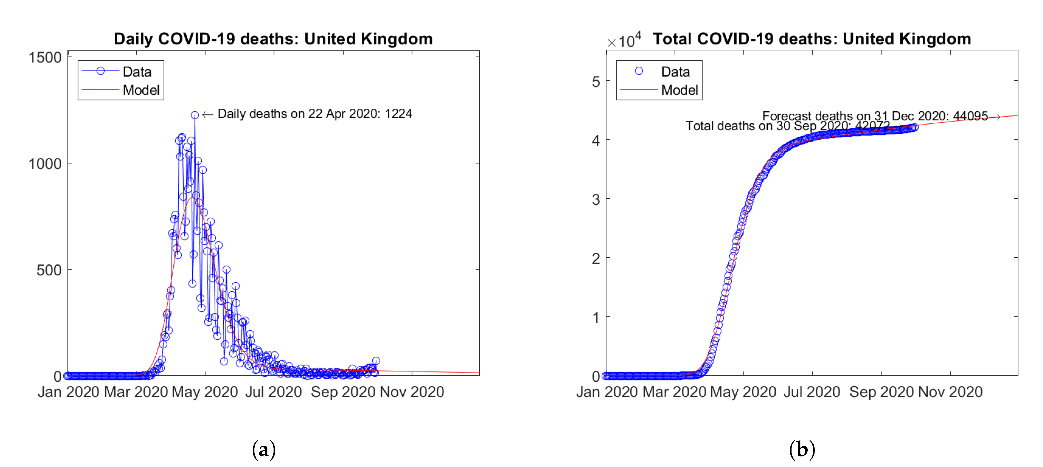
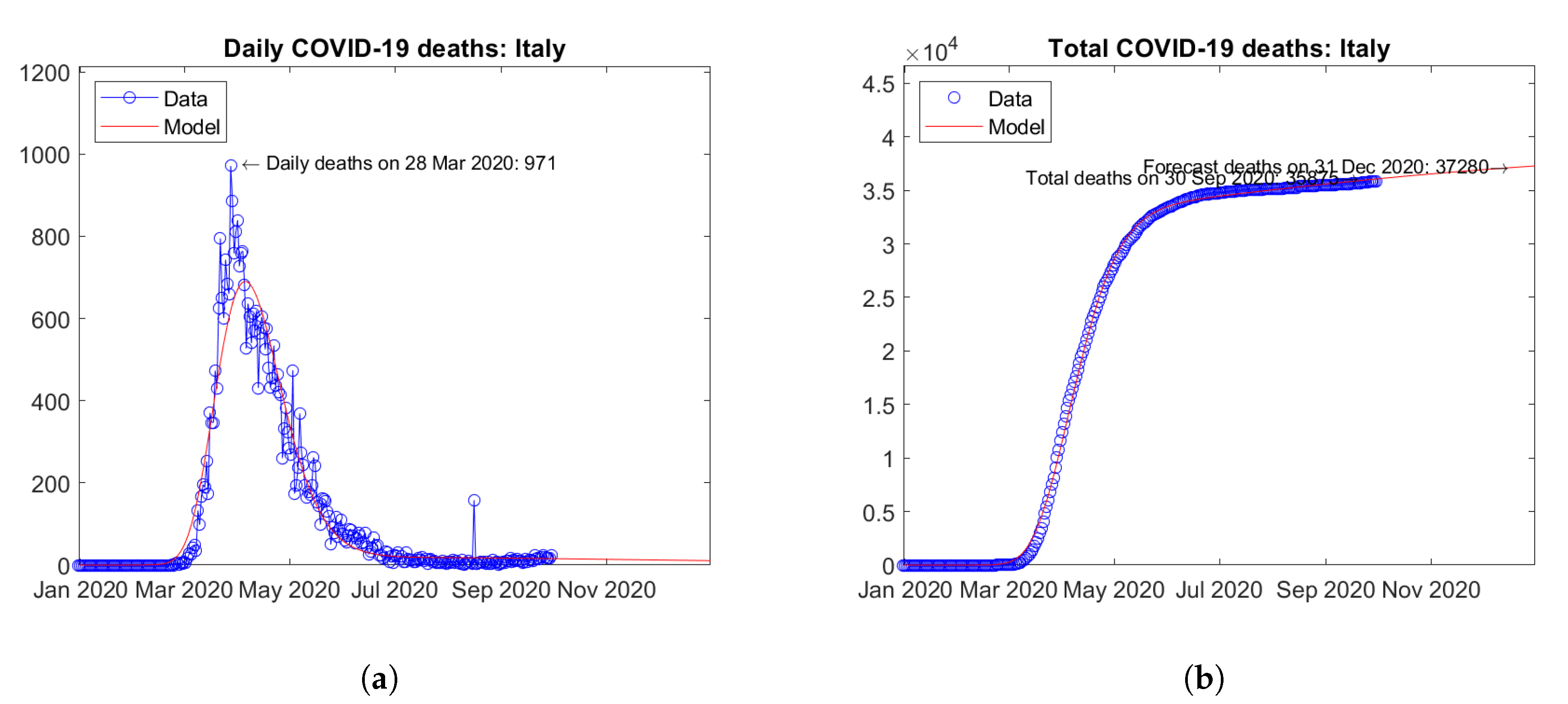
In Europe, the United Kingdom (Figure 10) and Italy (Figure 11) are the two countries with the largest number of actual and predicted COVID-19 deaths. Here, peaks of daily deaths were reported in April (Figure 10a) and March 2020 (Figure 11a), respectively. Since then, decreasing trends have been observed. Today, weak increases in the number of daily deaths can be observed, but with no evidence of a incipient second wave (in terms of deaths). For both countries, the model predicts weakly increasing trends of the total number of deaths (Figure 10b and Figure 11b).
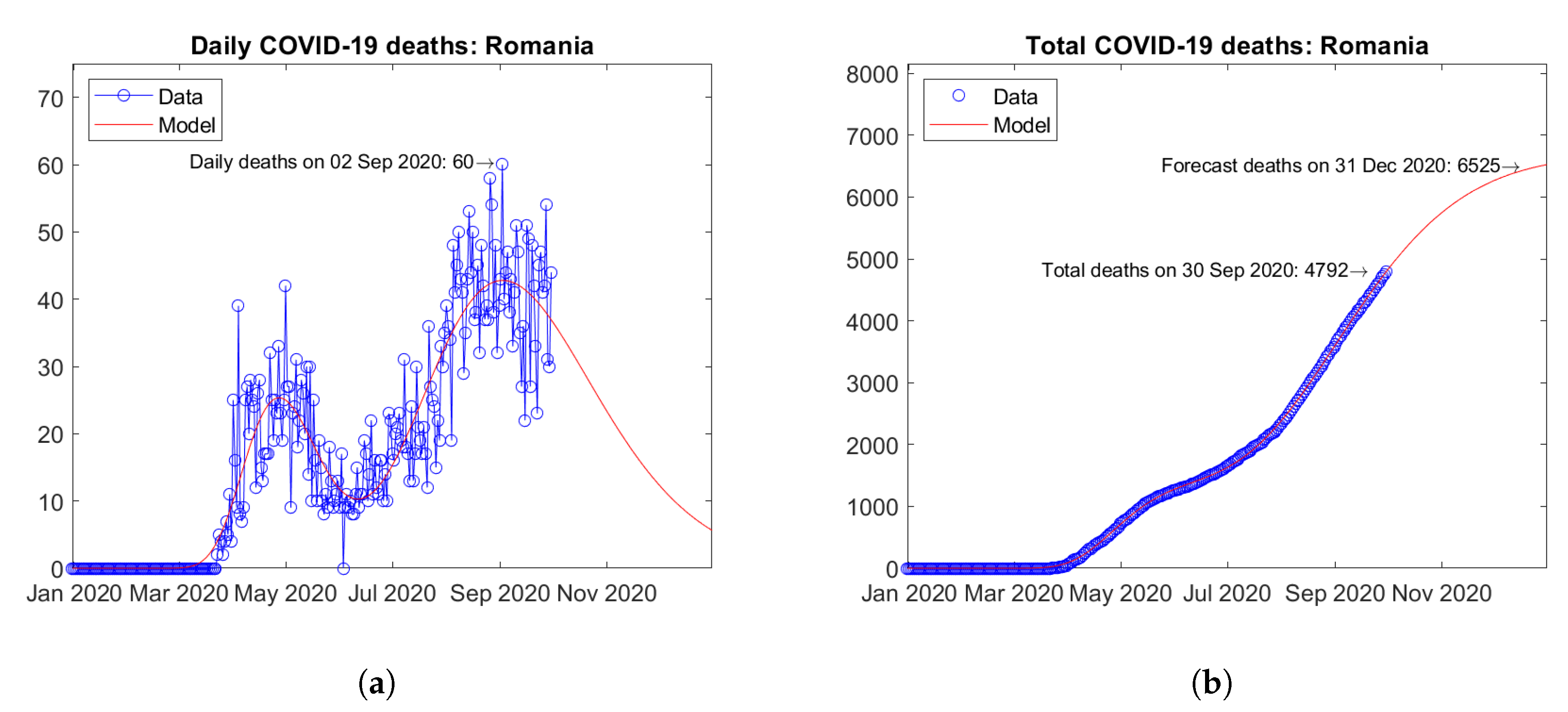
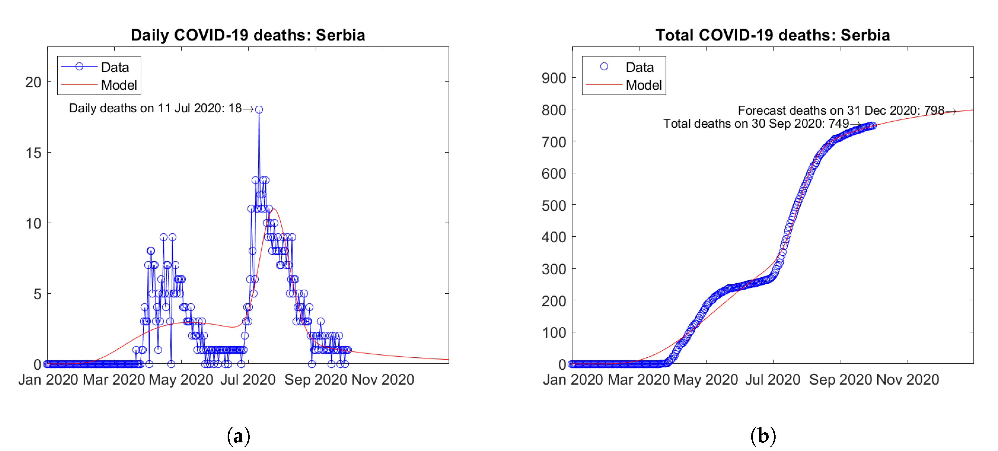
Some European countries were hit by second waves of the epidemic. For instance, in Romania (Figure 12) and Serbia (Figure 13), second peaks of daily deaths have been reported in September (Figure 12a) and July 2020 (Figure 13a), respectively. For both countries, increasing trends of the total number of deaths are predicted by the model (Figure 12b and Figure 13b).
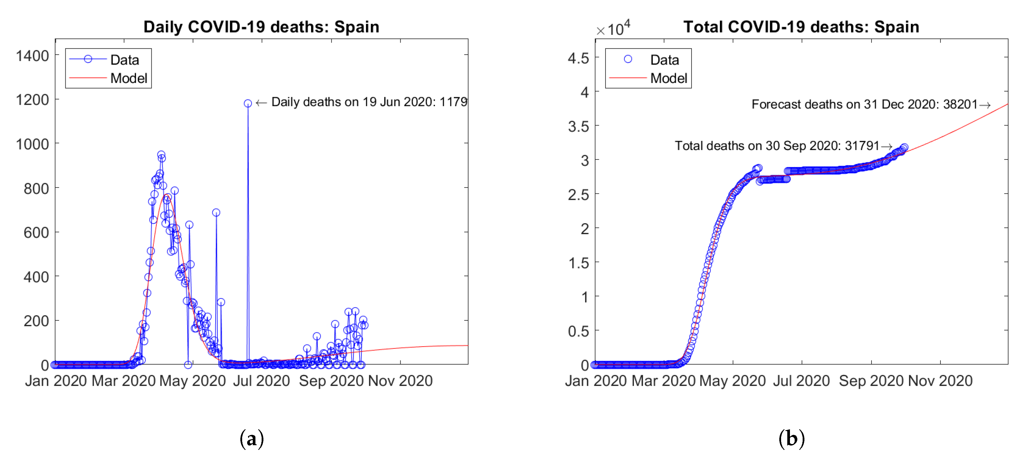
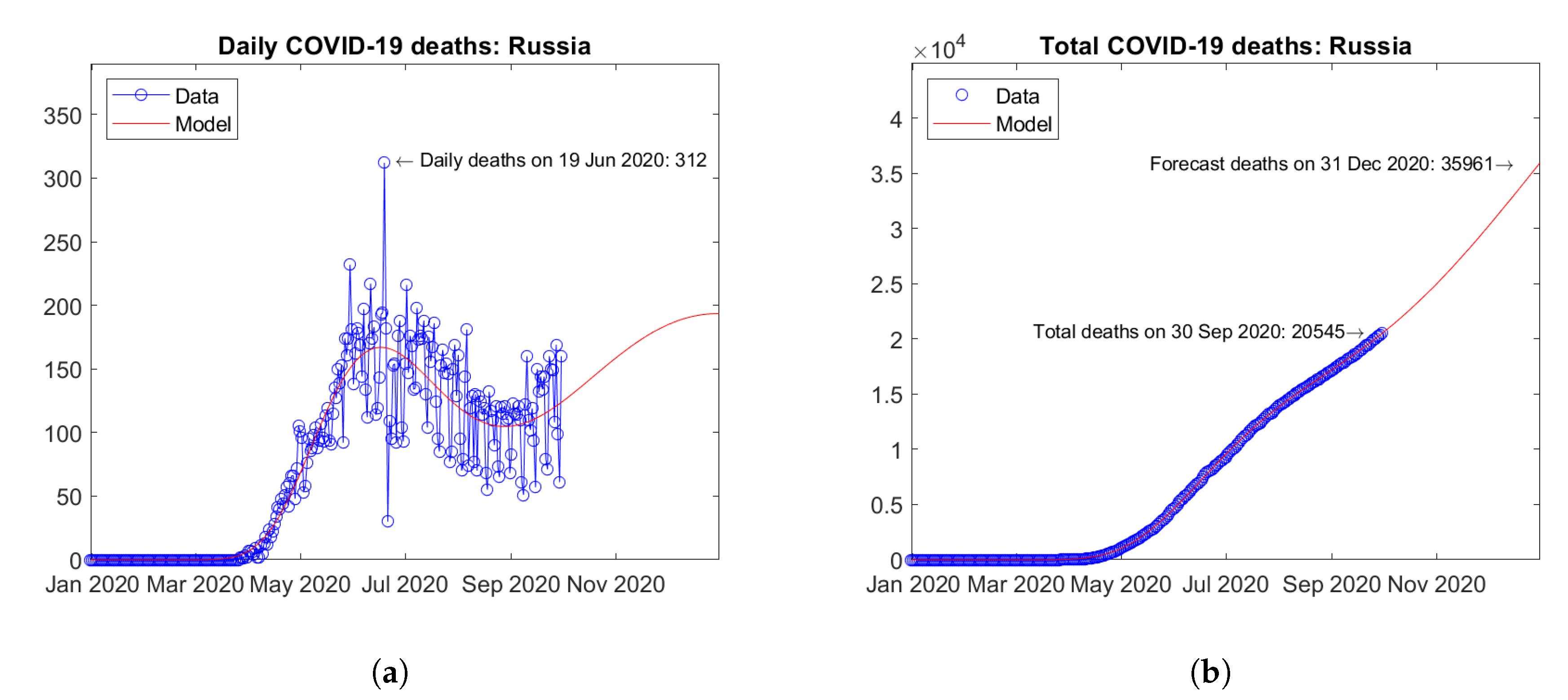
In other European countries, second waves of the epidemic have just started or are expected in the coming months. For instance, in Spain (Figure 14) and Russia (Figure 15), trends can be observed towards a second peak of daily deaths by the end of year 2020 (Figure 14a) and Figure 15a). For both countries, strongly increasing trends of the total number of deaths are predicted by the model (Figure 14b and Figure 15b).
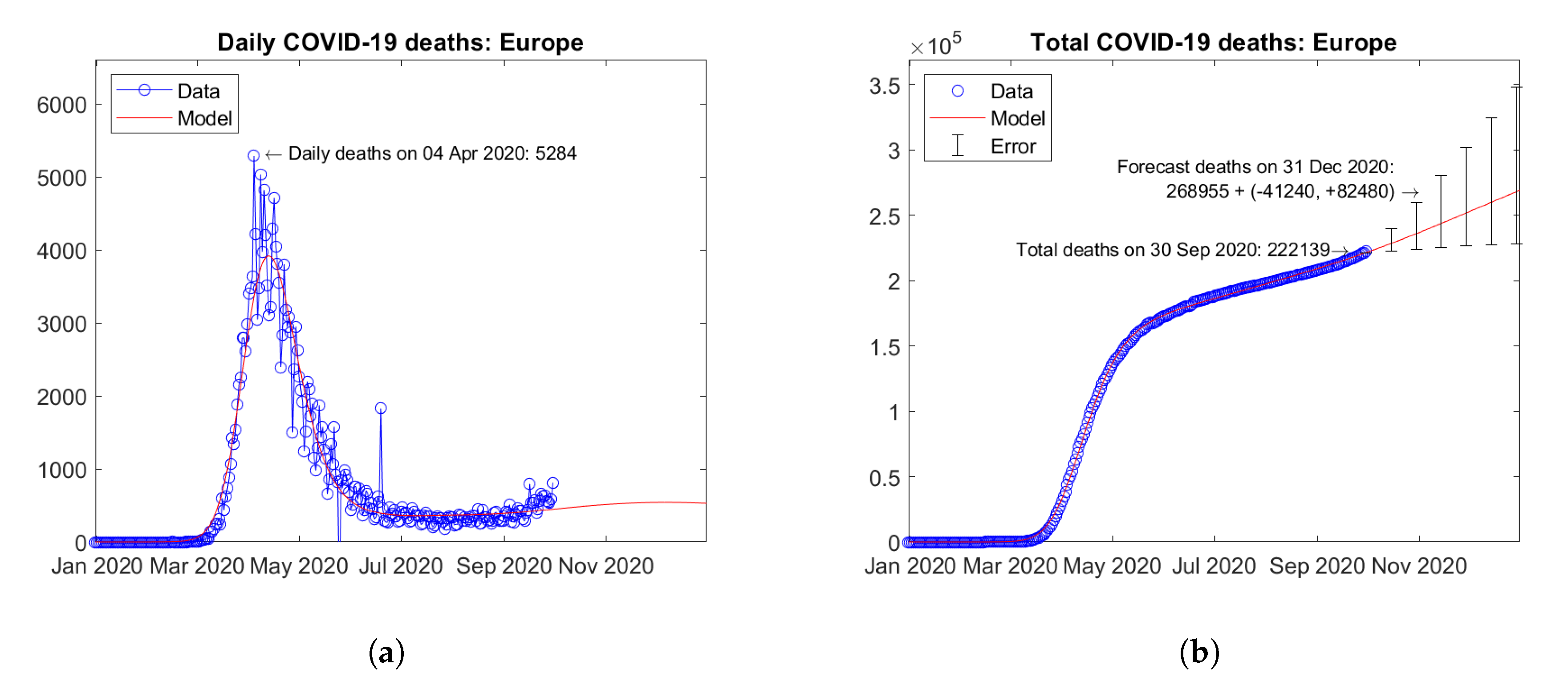
Figure 16 shows the time trends obtained for Europe by summing the available data and model predictions for each country. The overall trends are dominated by countries with the highest number of fatalities (United Kingdom, Italy, France, Spain, etc.). A slight tendency towards a second wave can be observed in the continental resume; however with a much lower estimated second peak with respect to April 2020 (Figure 16a). Figure 16b shows the actual and forecast number of total deaths in the continent. The predicted future trend is moderately increasing. Error bars correspond to the error rate (−2.5%, +5%)/15 days estimated through the validation study. The forecast total number of COVID-19 deaths on 31 December 2020 in Europe is 268,955 + (−41,240, +82,480).
5.3. North America
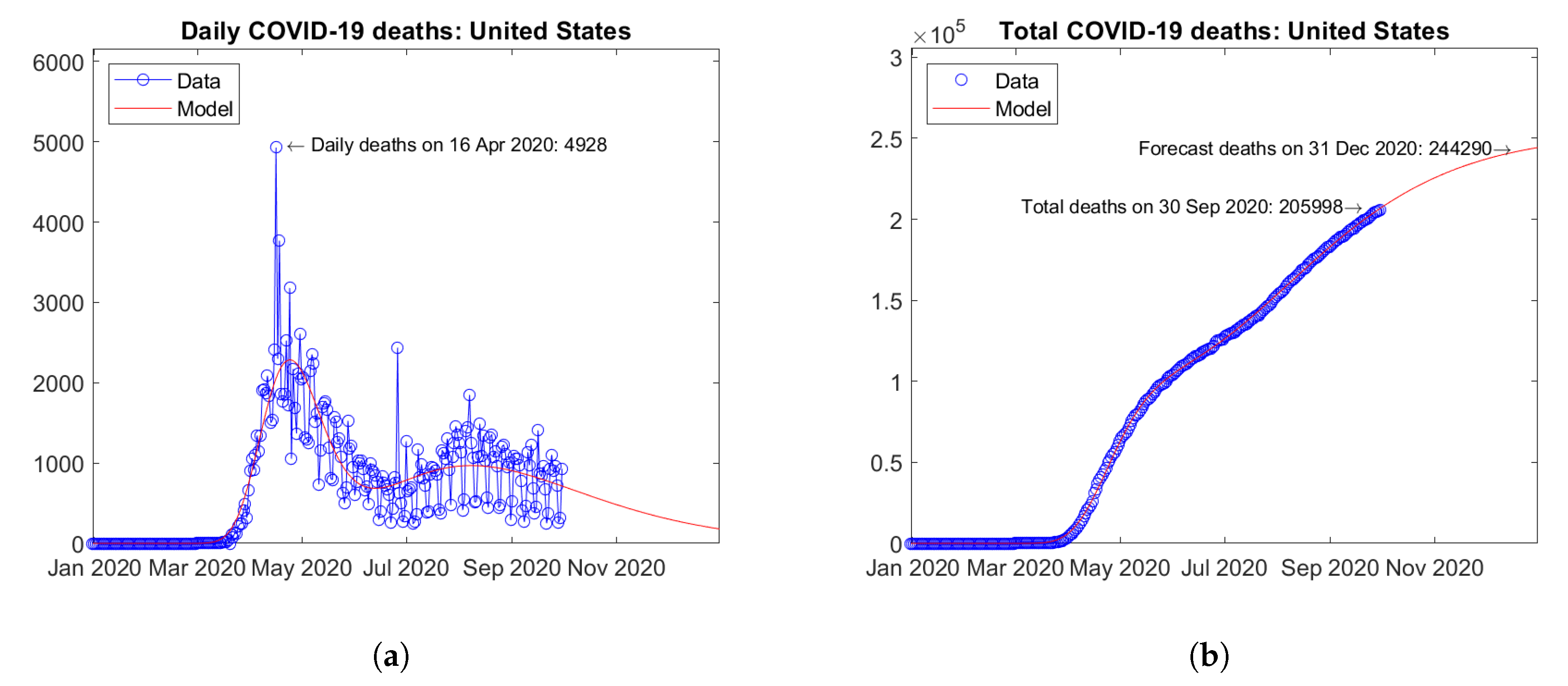
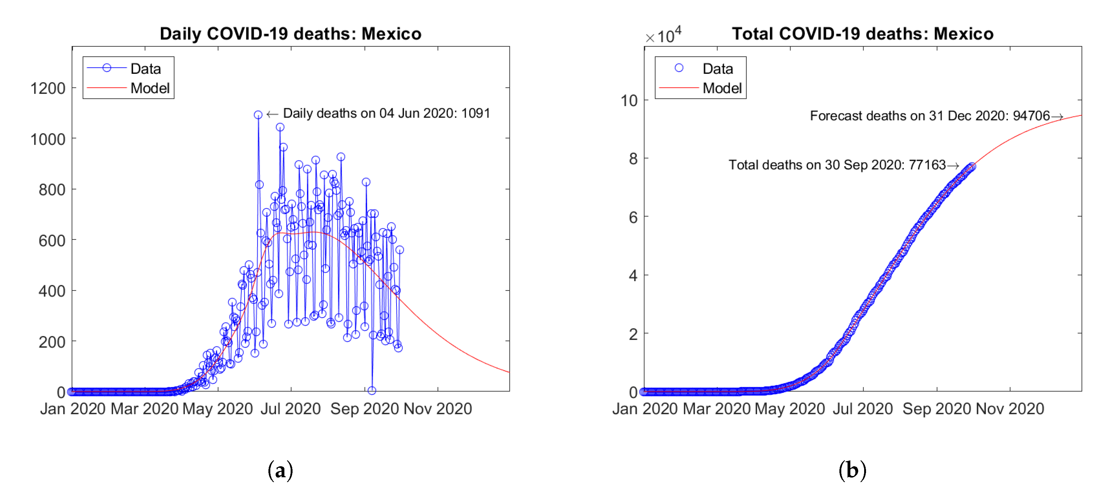
In North America, the United States (Figure 17) and Mexico (Figure 18) report the largest number of COVID-19 deaths. In the United States, the daily deaths reached a first peak in April and a second peak in August 2020 (Figure 17a). Mexico shows a different trend of daily deaths, with a plateau between June and August 2020 (Figure 18a). For both countries, the model predicts increasing trends of the total number of deaths (Figure 17b and Figure 18b).
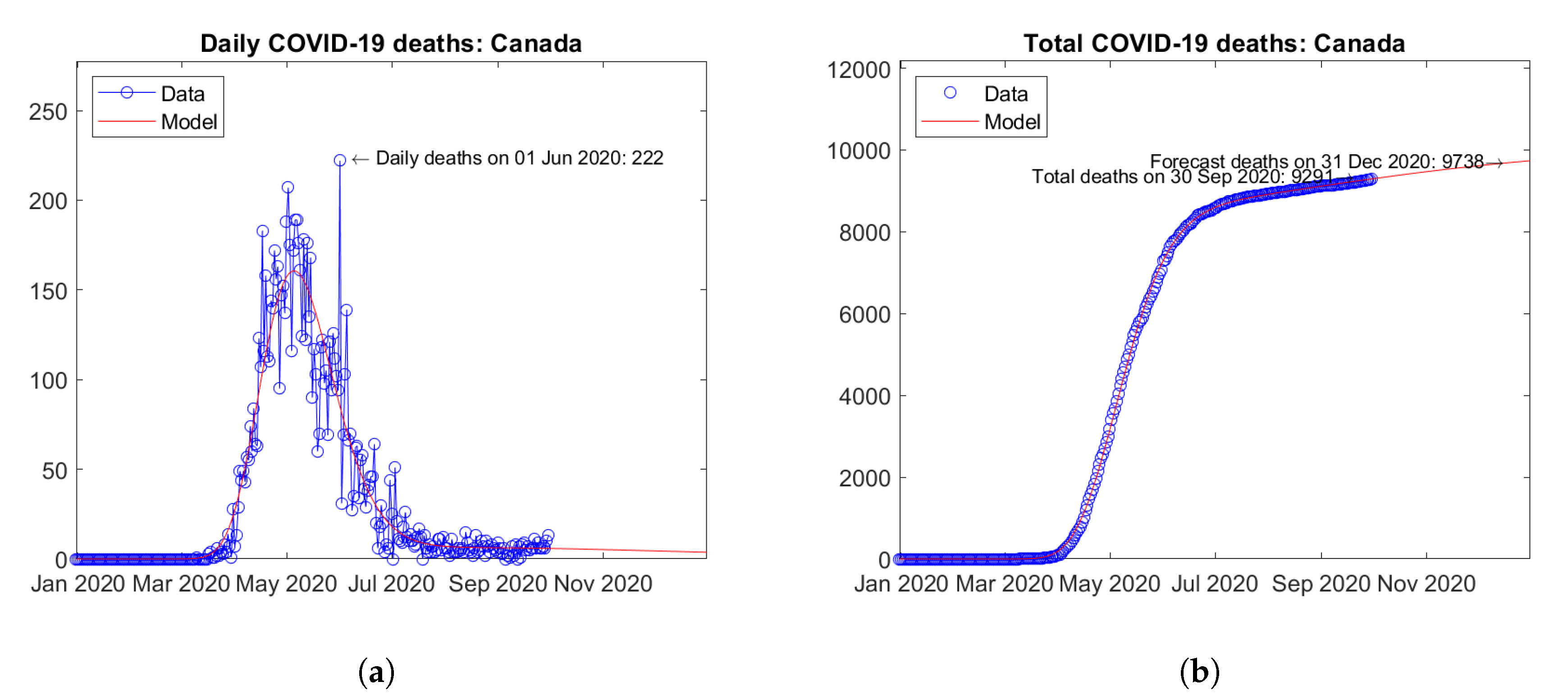
Figure 19 summarizes the results for Canada. The trends of the daily (Figure 19a) and total (Figure 19b) number of deaths are similar to many European countries with no visible signs of second waves.
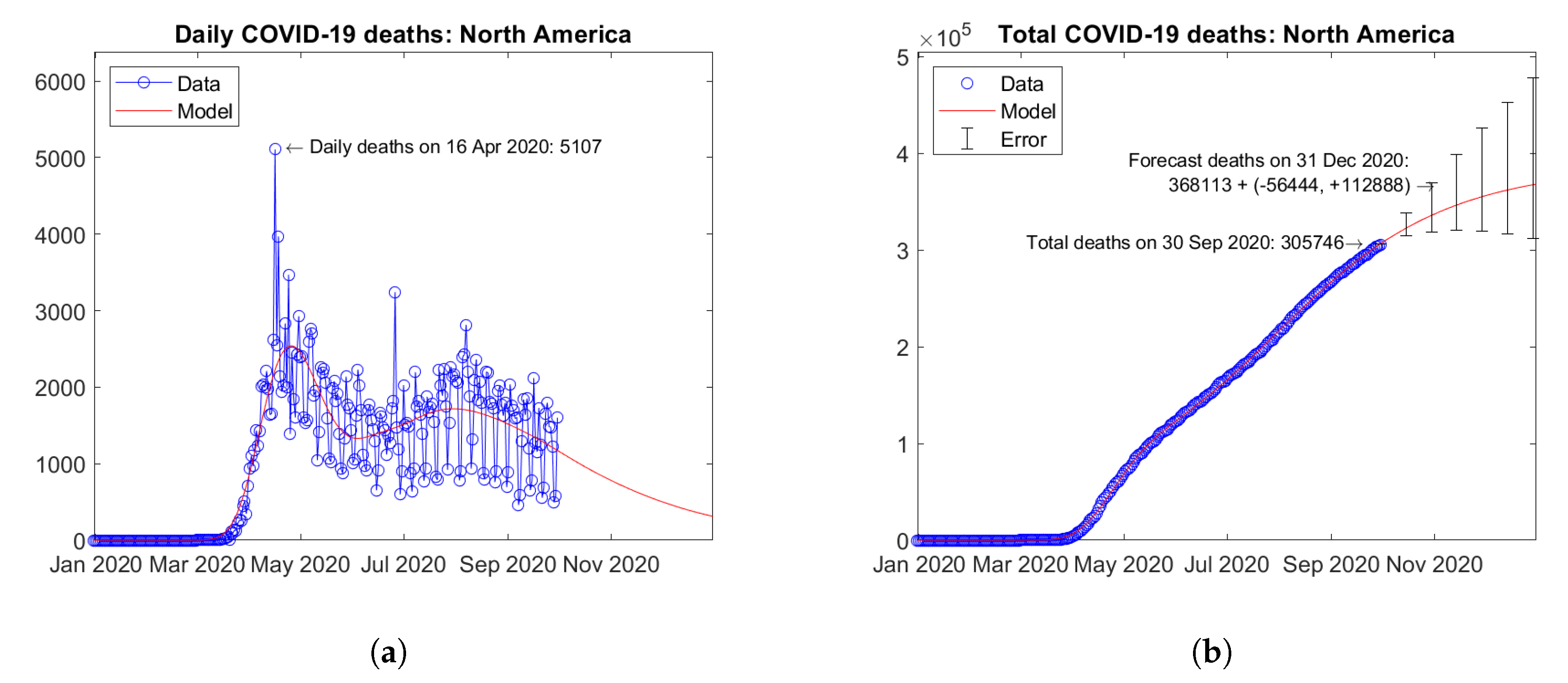
Figure 20 shows the time trends obtained for the North American continent by summing the available data and model predictions for each country. The overall trends are dominated by countries with the highest number of fatalities (United States and Mexico). A second wave is visible in current data with a peak in August 2020 (Figure 20a). Figure 20b shows the actual and forecast number of total deaths in the continent. The predicted future trend is moderately increasing. Error bars correspond to the error rate (−2.5%, +5%)/15 days estimated through the validation study. The forecast total number of COVID-19 deaths on 31 December 2020 in North America is 368,113 + (−56,444, +112,888).
5.4. South America
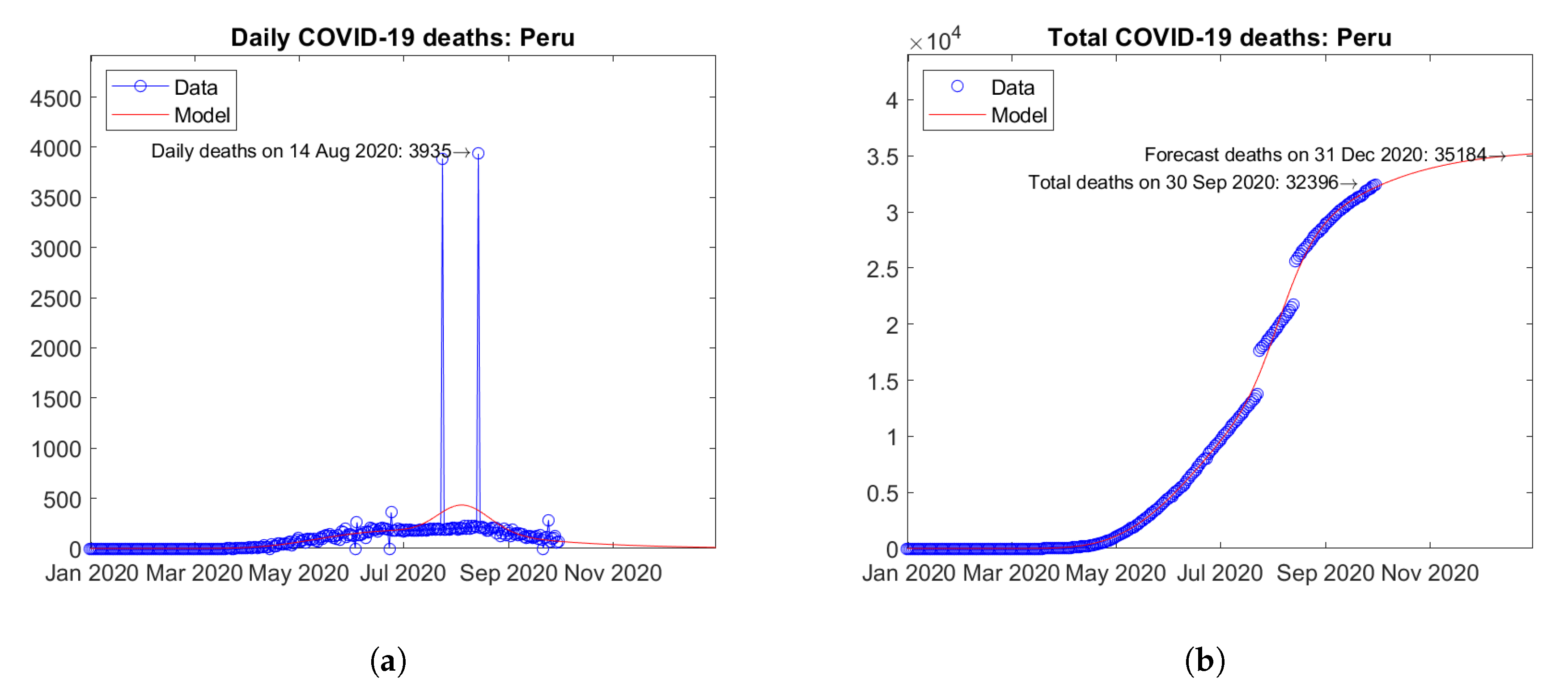
In South America, Brazil (Figure 21) and Peru (Figure 22) are the two countries with the largest number of actual COVID-19 deaths. In Brazil, the number of daily deaths has undergone a sort of plateau from June to August 2020, followed by a descending branch (Figure 21a). In Peru, the official data on daily deaths show two isolated peaks, which the model fits smoothly with a single maximum (Figure 22a). For both countries, the model predicts increasing trends of the total number of deaths (Figure 21b and Figure 22b).
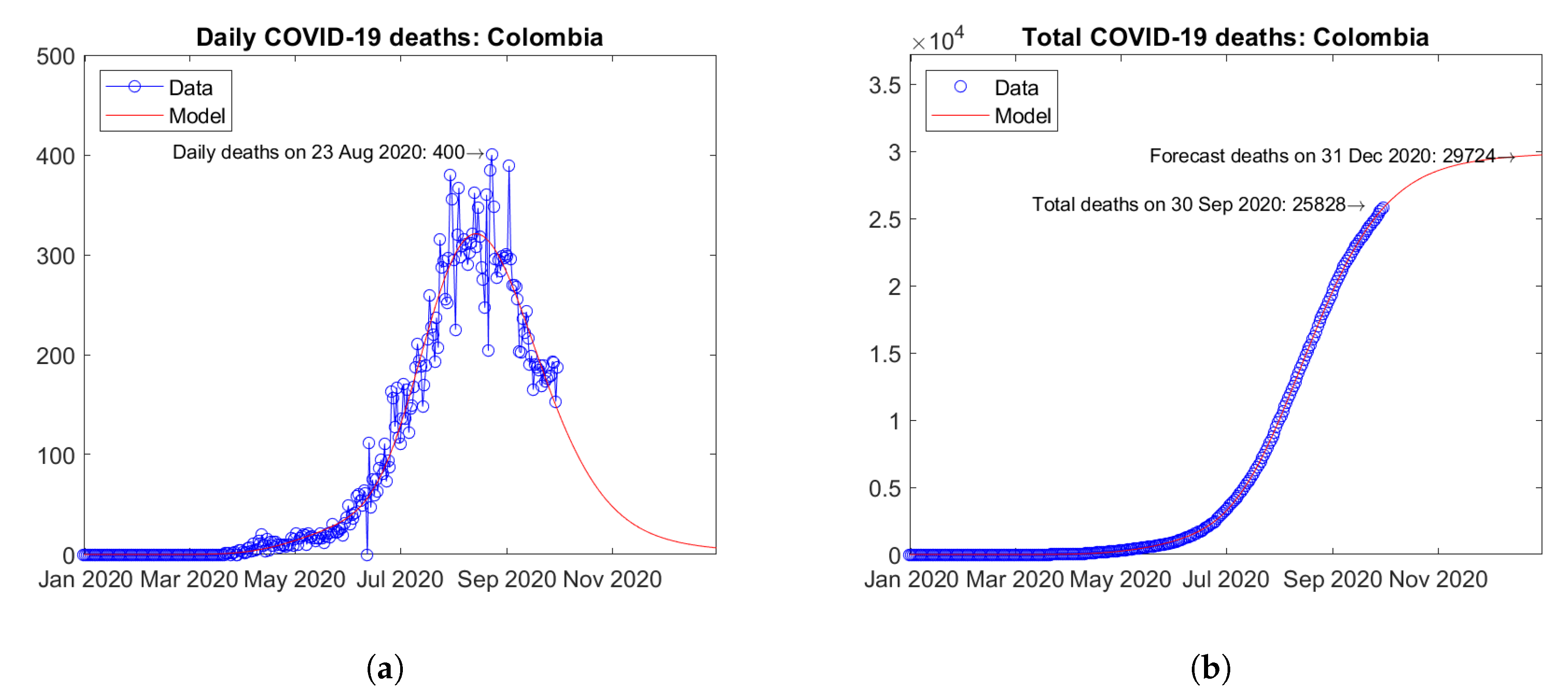
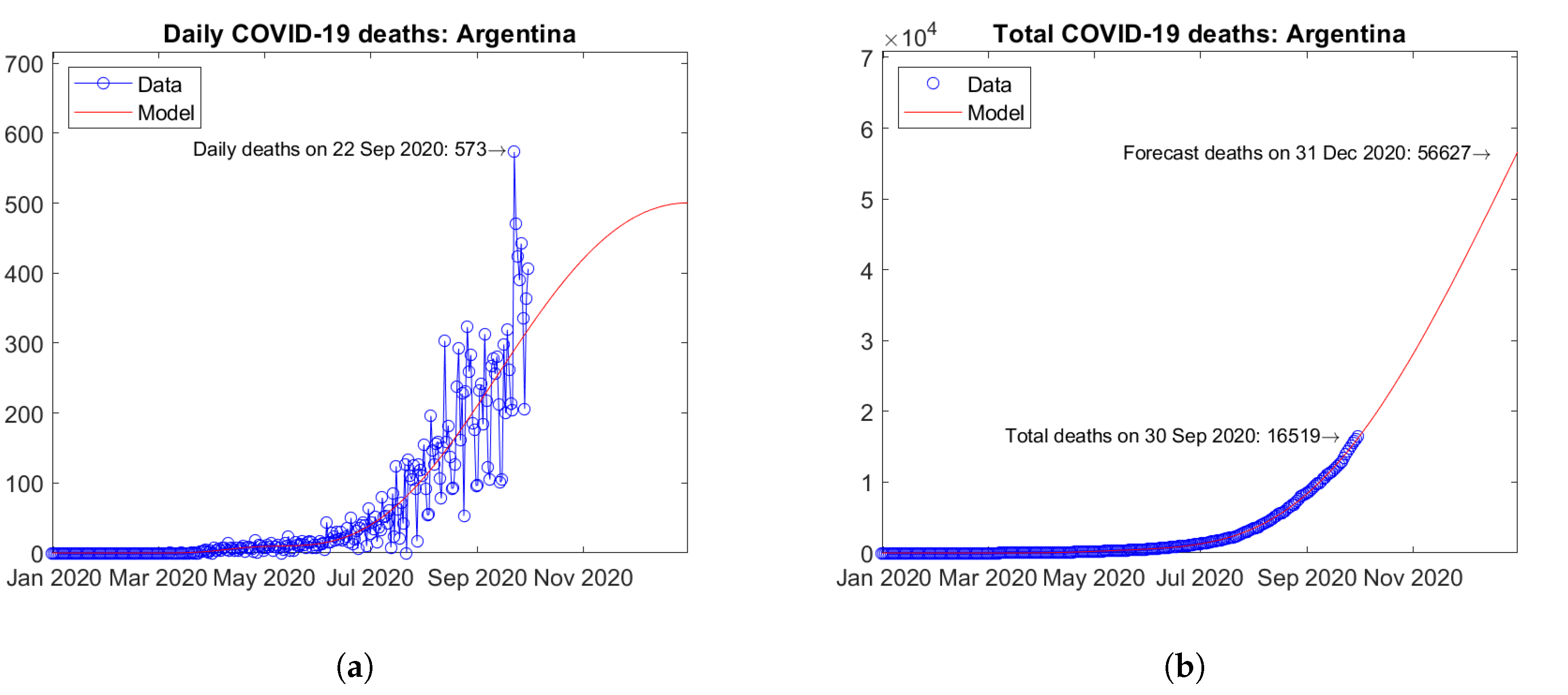
The third and fourth South American countries for the total number of COVID-19 deaths are Colombia (Figure 23) and Argentina (Figure 24). In Colombia, the number of daily deaths experienced a peak in August 2020, followed by a descending trend (Figure 23a). In Argentina, the epidemic seems to be still at an early stage and the first peak of daily deaths has not been reached yet (Figure 24a). The model predicts a moderately increasing trend of the total number of deaths for Colombia (Figure 23b) and a strongly increasing trend for Argentina (Figure 24b).
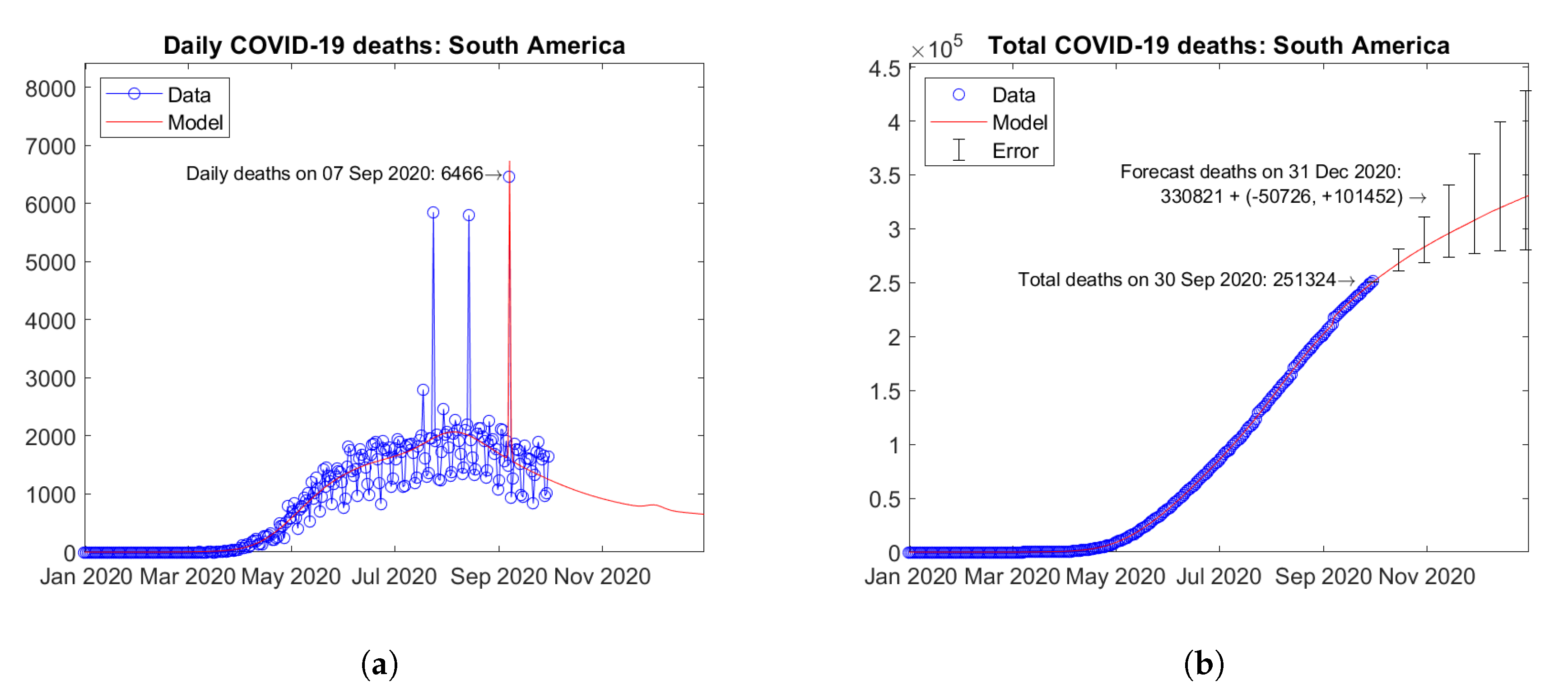
Figure 25 shows the time trends obtained for the whole South America by summing the available data and model predictions for each country. According to the model, the daily number of deaths is expected to undergo a descending trend in the next months (Figure 25a). Figure 25b shows the actual and forecast number of total deaths in the continent. The predicted future trend is moderately increasing. Error bars correspond to the error rate (−2.5%, +5%)/15 days estimated through the validation study. The forecast total number of COVID-19 deaths on 31 December 2020 in South America is 330,821 + (−50,726, +101,452).
5.5. Africa
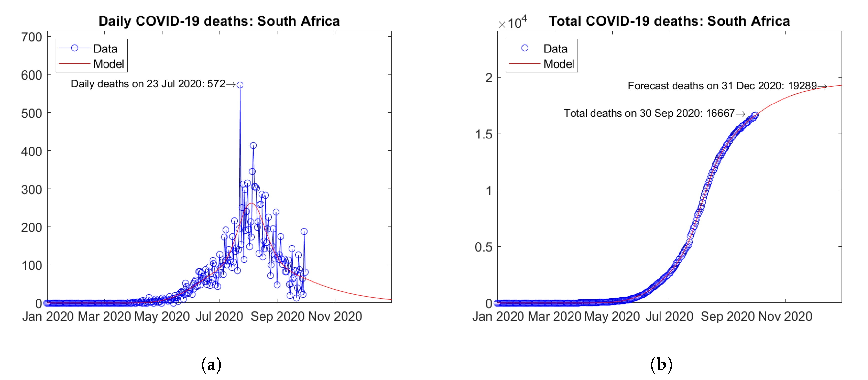
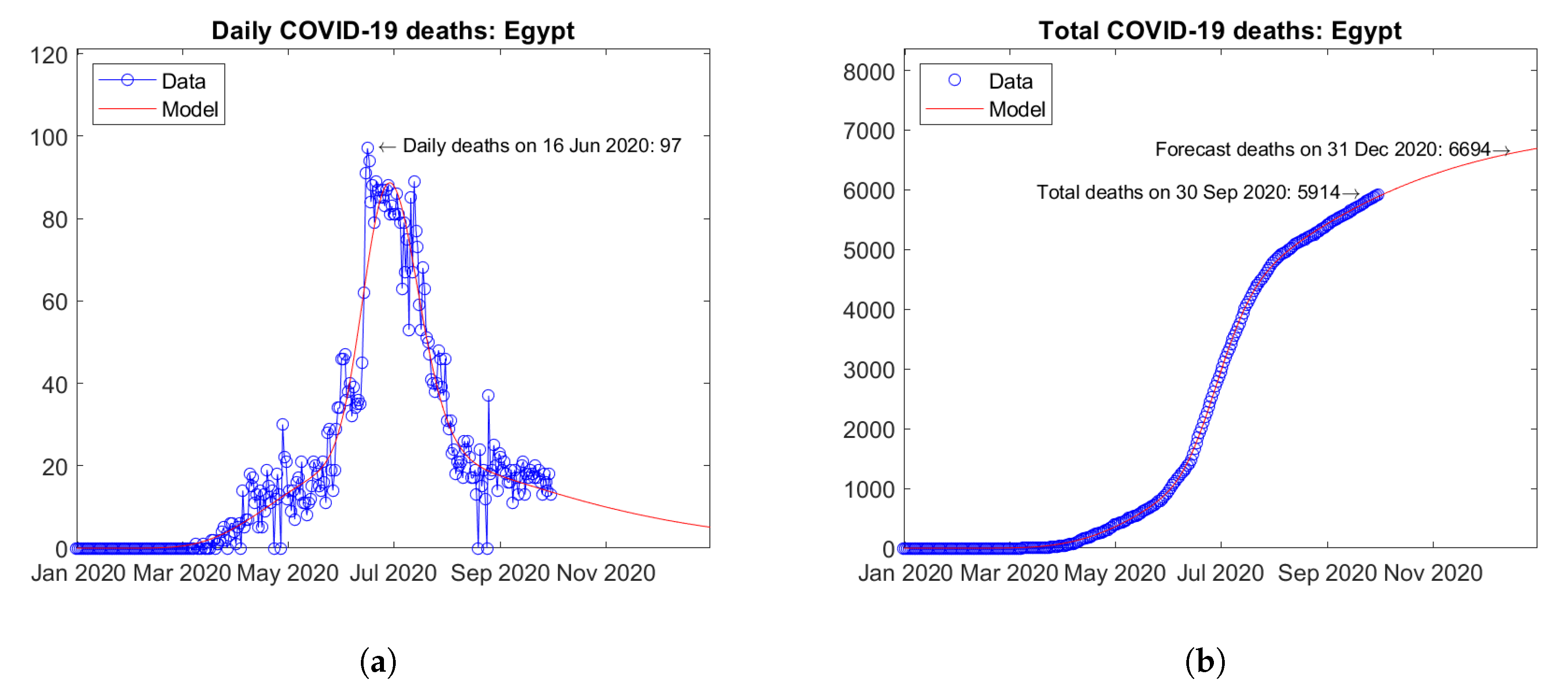
South Africa (Figure 26) and Egypt (Figure 27) are the two African countries with the largest number of actual COVID-19 deaths. In both countries, peaks of daily deaths have been reached and the predicted future trends are descending with no visible second waves (Figure 26a and Figure 27a). The predicted total number of deaths show moderately increasing trends (Figure 26b and Figure 27b).
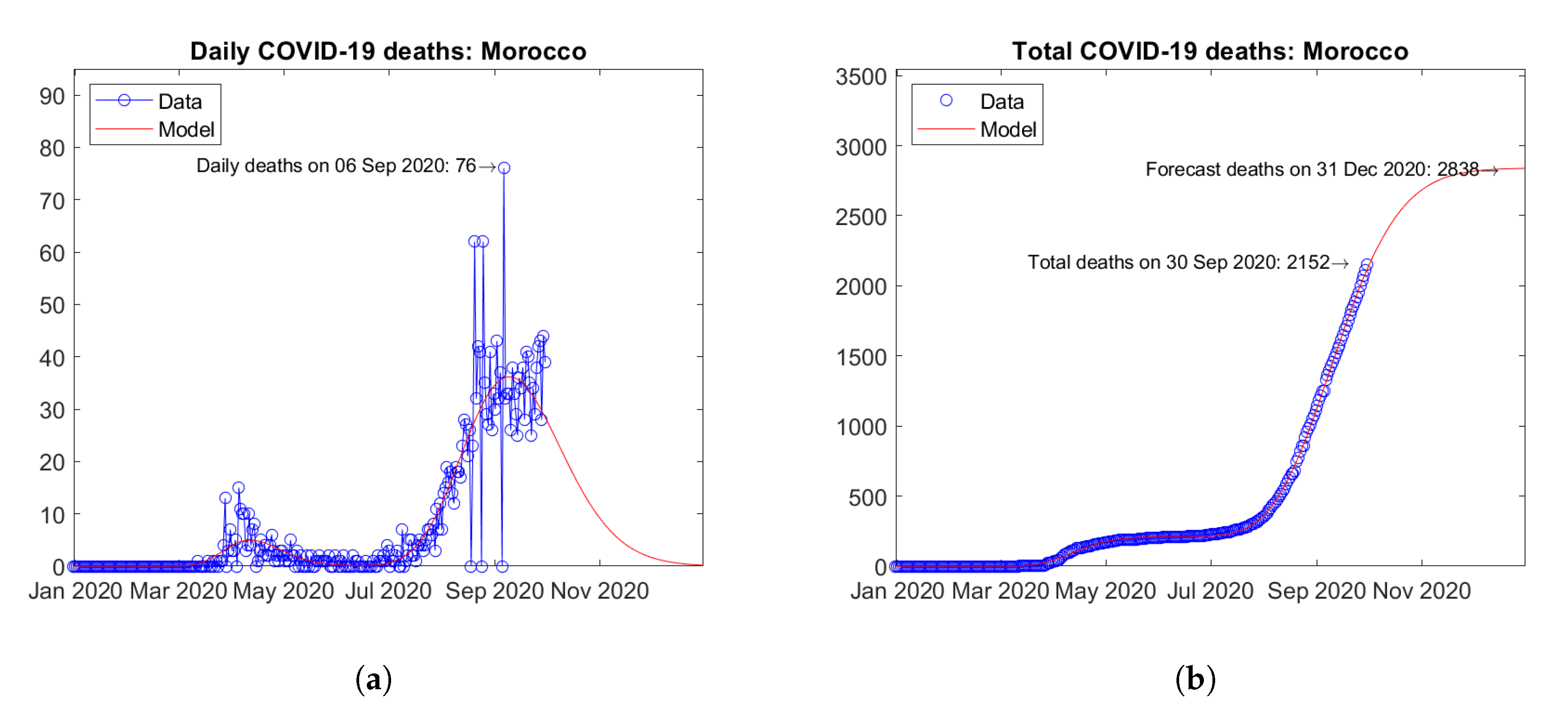
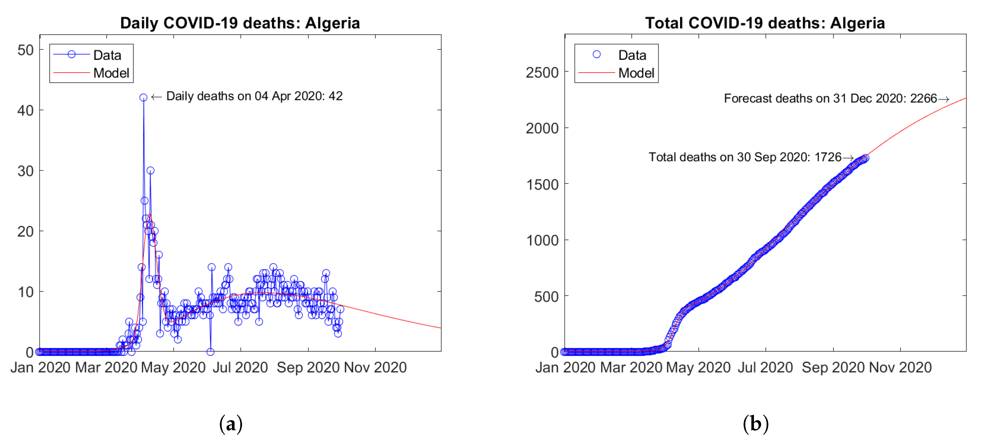
Morocco (Figure 28) Algeria (Figure 29) respectively are the third and fourth African countries with the largest number of predicted COVID-19 deaths. In both countries, a first peak of daily deaths occurred in April 2020, followed by a second wave with a new peak around September 2020 (Figure 28a and Figure 29a). The model predicts increasing trends of the total number of deaths (Figure 28b and Figure 29b).
Figure 30 shows the time trends obtained for Africa by summing the available data and model predictions for each country. The daily number of deaths is currently on a descending trend (Figure 30a). Figure 30b shows the actual and forecast number of total deaths in the continent. The predicted future trend is strongly increasing. Error bars correspond to the error rate (−2.5%, +5%)/15 days estimated through the validation study. The forecast total number of COVID-19 deaths on 31 December 2020 in Africa is 45,723 + (−7011, +14,022).
5.6. Oceania
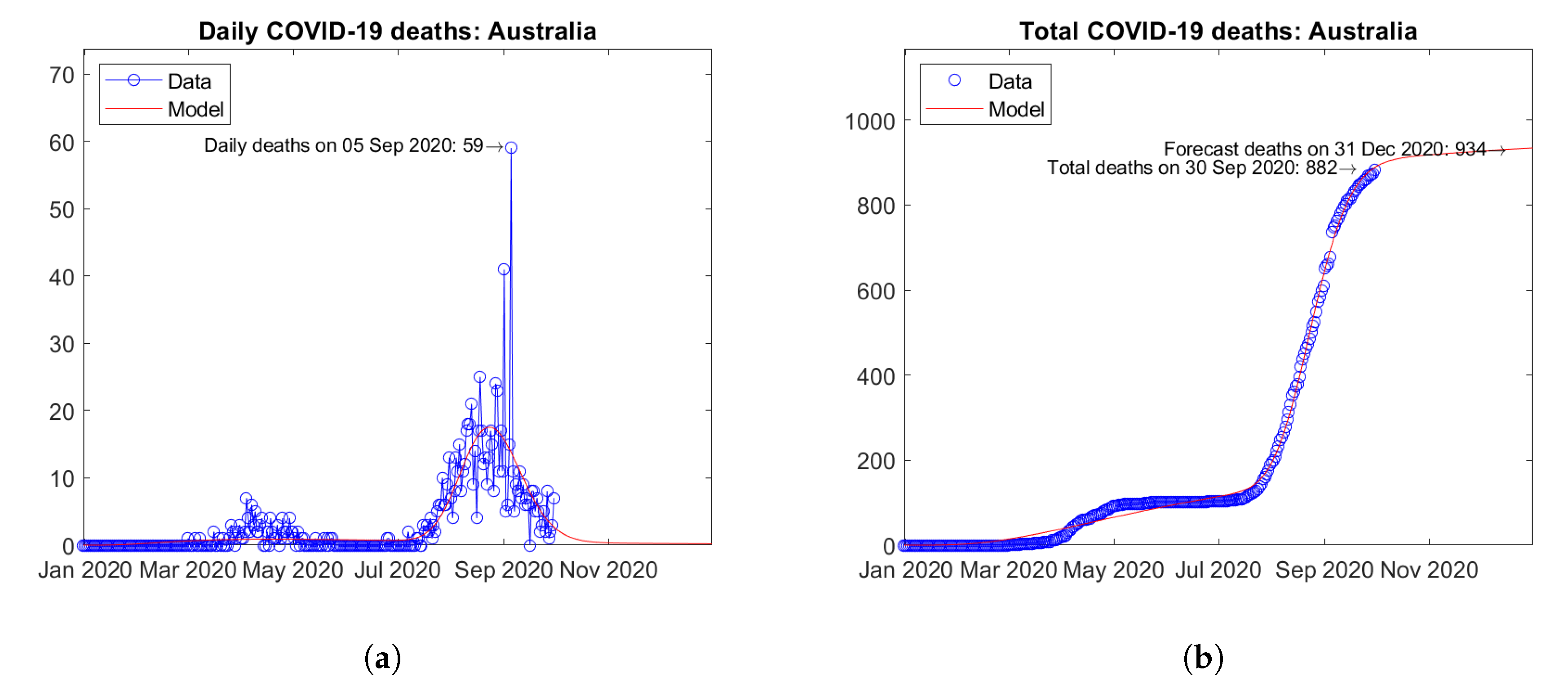
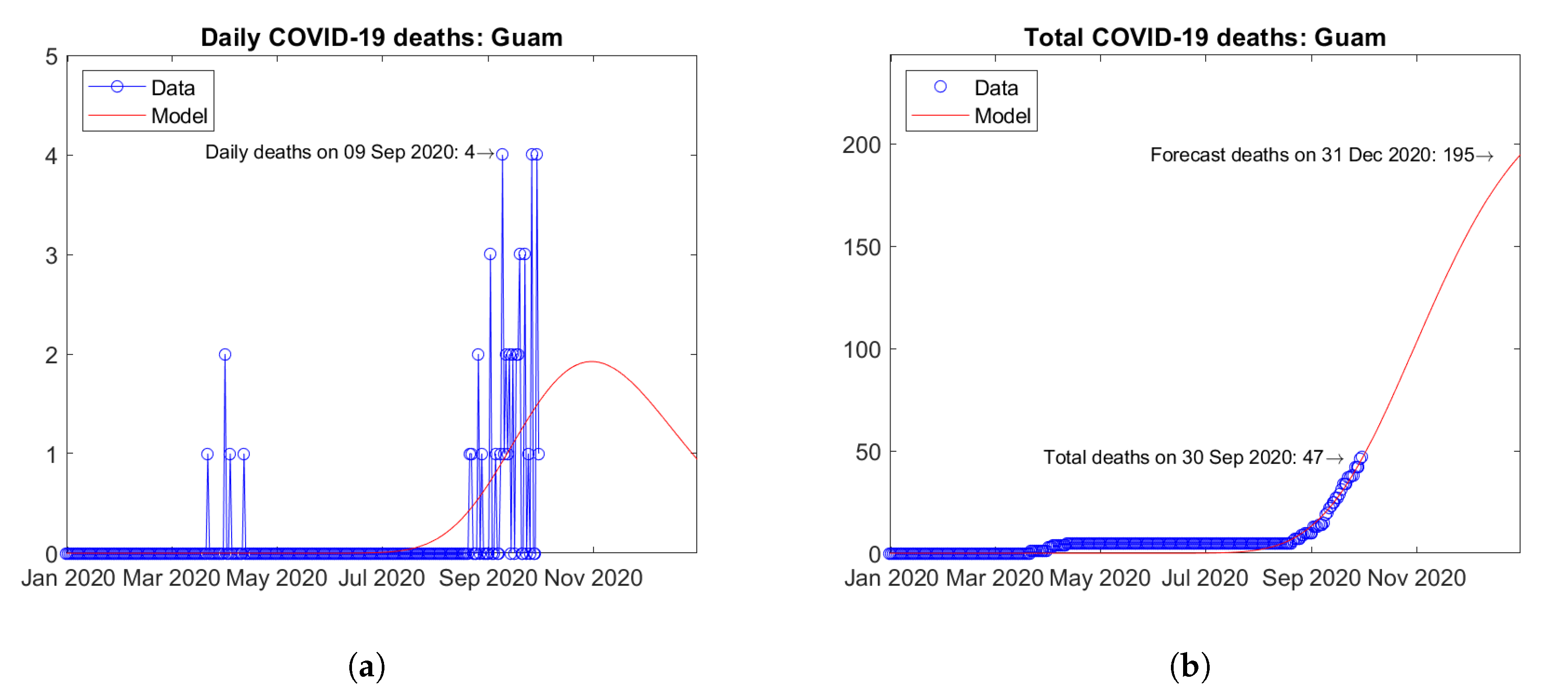
In Oceania, Australia (Figure 31) and Guam (Figure 32) are the two countries with the largest number of COVID-19 deaths. Both countries experienced a first peak of daily deaths in April 2020, followed by a second wave with a new peak in September 2020 (Figure 31a and Figure 32a). The predicted total number of deaths are weakly increasing (Figure 31b and Figure 32b).
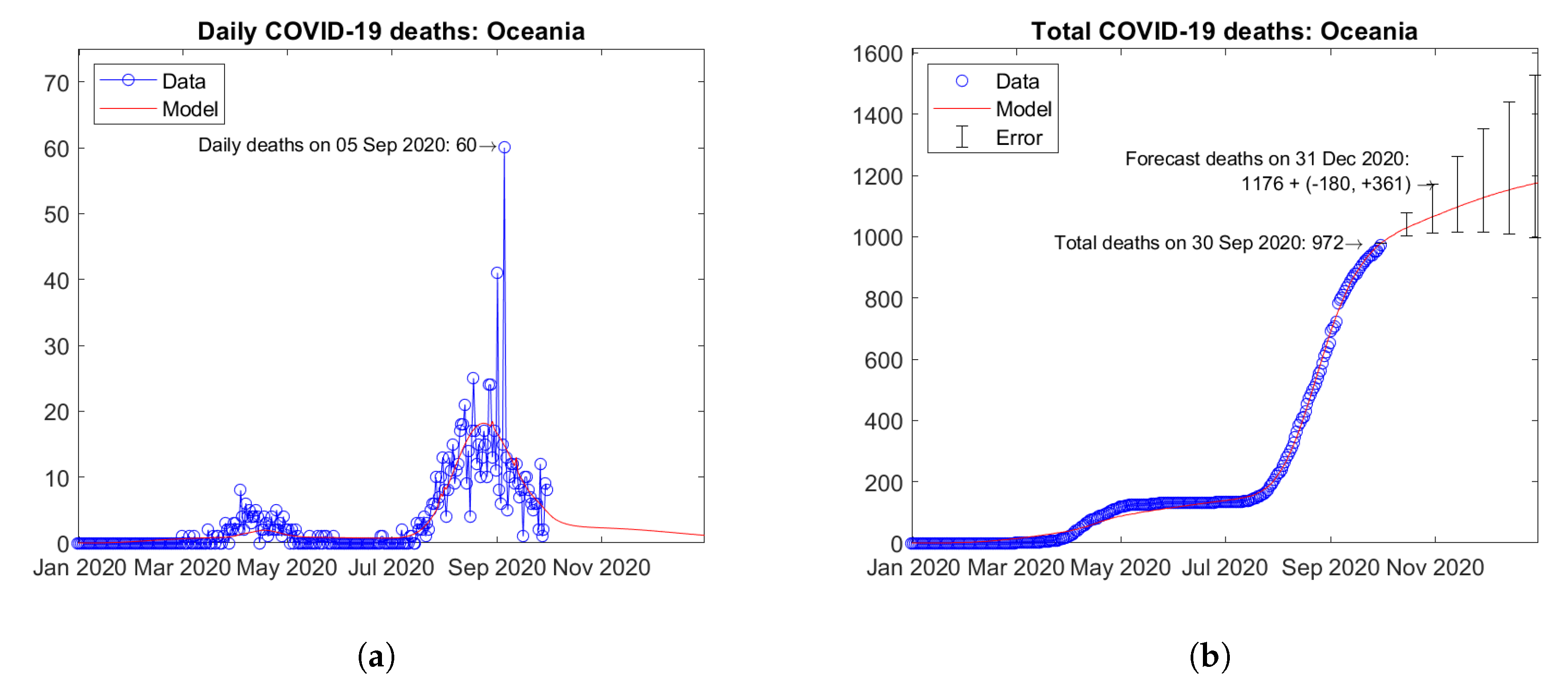
Figure 33 shows the time trends obtained for Oceania by summing the available data and model predictions for each country. The continental trends are strongly dominated by the contribution of Australia. A second wave is currently ongoing, but the predicted trend of daily deaths is descending (Figure 33a). Figure 33b shows the actual and forecast number of total deaths in the continent. The predicted future trend is weakly increasing. Error bars correspond to the error rate (−2.5%, +5%)/15 days estimated through the validation study. The forecast total number of COVID-19 deaths on 31 December 2020 in Oceania is 1176 + (−180, +361).
5.7. World
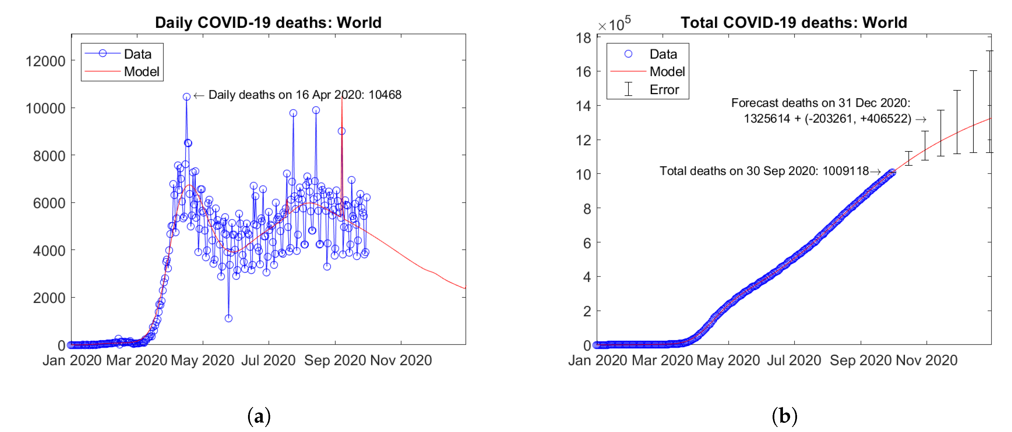
Figure 34 shows the time trends obtained for the whole World by summing the available data and model predictions for all of the available countries. After a first peak of daily deaths in April 2020, a second wave of the pandemic is ongoing with a second peak in August 2020. The predicted trend of daily deaths is slowly decreasing (Figure 34a). Figure 34b shows the actual and forecast number of total deaths. The predicted future trend is moderately increasing. Error bars correspond to the error rate (−2.5%, +5%)/15 days estimated through the validation study. The forecast total number of COVID-19 deaths on 31 December 2020 in the World is 1,325,614 + (−203,261, +406,522).
6. Discussion
6.1. Parameter Identifiability
A relevant issue of epidemiological models is the identifiability of their parameters. In particular, structural identifiability concerns the well-posedeness of the mathematical problem, while practical identifiability is related to the possibility of estimating the parameter values based on the available data [22]. Several methods have been developed to assess the parameter identifiability in models formulated in terms of differential equations to be solved numerically [23]. The present model is formulated instead in terms of assumed analytical expressions, namely Equations (1) and (2), which include six parameters (A, , , , , and ) for each country. Assuming, without loss of generality, that (and excluding the degenerate case, where the two lognormal distributions overlap onto a single distribution), any set of parameter values can be uniquely mapped to a model output. Thus, the present model is structurally identifiable [24]. The model is also practically identifiable, as proven by the successful computation of parameters through the implemented data fitting procedure.
6.2. Observed Trends
The COVID-19 pandemic is affecting different regions around the World in different ways at different times. This is reflected in the different trends observed for the countries and continents presented in the previous Section.
In some countries (e.g., Argentina and—not shown in the paper, but available in the Supplementary Materials—Venezuela, as well as many African countries), the epidemic is still at an initial stage of exponential growth. Other countries (e.g., India, Mexico, and Brazil) are currently facing the first wave, while other ones (e.g., Peru, Colombia, South Africa, and Egypt) are on the tail of the first wave. In many European countries (e.g., United Kingdom and Italy), as well as in China and Canada, the first wave has been completely overcome. In some countries (e.g., Spain and Russia), more or less evident signs of a second incipient wave can be observed. Other countries (e.g., Israel, Romania, United States, Morocco, Algeria, and Guam) are currently facing a second wave of the epidemic. Other ones (e.g., Japan, Serbia, and Australia) are already at the tail of the second wave. Lastly, in Iran, a third wave of the epidemic is currently going on.
It should be observed that, in large federal nations, the trends of daily deaths observed at the national level are actually the sum of many local trends occurring in the single federated states. This could explain the plateau shapes observed in the daily deaths plots of Brazil and Mexico. Likewise, the second wave observed in the plot of the United States could correspond actually to a first wave of the epidemic affecting a different area of the country. For the above-mentioned countries, more accurate data fitting and extrapolations could be obtained by scaling down the model to consider the statistical data of single states and then accumulating the results at national level.
In any case—except maybe for Iran, because of the incipient third wave-, the bimodal lognormal time distribution of daily deaths assumed by the model was able to fit with reasonable accuracy the observed data.
6.3. Computational Efficiency
As of 30 September, 275 data points (day, number of total deaths) are processed for each location, for a total of data points to be fitted. The model has 6 parameters for each of the 211 locations in the OWID dataset. Thus, parameters are determined overall. The fitting procedure runs in less than 2 min on an ordinary personal computer.
6.4. Representativeness of Predictions
The fitted data are the official number of deaths reported by national health agencies worldwide. Thus, also the predictions of the model obtained through extrapolation should be interpreted as a forecast of the official number of reported deaths. It is difficult to state whether the real number of COVID-19 deaths is well represented by the model. For instance, in some European countries, such as Italy and the United Kingdom, it has been reported that official statistics may have underestimated the real number of deaths. Even more so, the same situation can be expected for many developing countries.
Some insight can be obtained by looking at the fatality rates. Table 4 reports the actual and predicted fatality rates for the six continents and the World. The fatality rates of Africa, Asia, and Oceania are one order of magnitude smaller than those of Europe and the Americas. This could be a sign of an underestimation of official reports with respect to real data in such continents. The fatality rates of North and South America are about twice the values of Europe. This could be due to the different lockdown measures imposed by national governments in the compared continents.
7. Conclusions
A phenomenological epidemiological model has been presented for the description and prediction of COVID-19 deaths worldwide. The model assumes a bimodal lognormal distribution for the number of daily deaths in time in each country. Thanks to the asymmetry of the lognormal distribution function, the model is able to fit the available data better than other phenomenological models based on either the logistic or Gaussian distribution functions. Furthermore, thanks to the presence of a second mode in the time distribution, the model is able to describe the trends observed in countries hit by second waves of the epidemic. Besides, if a second wave is at an early stage of development, the model can estimate the time position of its peak.
The model has been validated by using the available data to predict retrospectively the known number of deaths on 30 September 2020. Thus, an estimate has been obtained of the error rate for the extrapolation of future trends. The forecast number of official deaths due to COVID-19 on 31 December 2020 in the World has been estimated at 1,325,614 + (−203,261, +406,522).
The proposed model is purely phenomenological. Thus, it cannot be used to predict the effects of any change of government policies or human behaviour. To this aim, transmission dynamics models should be used instead. Some transmission dynamics models only require a few parameters, while other ones require the specification of a large number of parameters, sometimes difficult to quantify. In the latter case, the numerical implementation of transmission dynamics models may be computationally very expensive. Conversely, the proposed model proved to be computationally very effective. It is able to process a large amount of (publicly available) data from more than two hundred countries and provide extrapolations in a few minutes by using a common personal computer.
To sum up, notwithstanding some obvious limitations due to the adopted approach, it is believed that the proposed model can be useful to forecast the trends of COVID-19 mortality in the short-to-medium term in a business-as-usual scenario. The computational effectiveness and the demand for only publicly available data are undoubted strengths of the proposed strategy.
Some future developments of the present work may be envisaged:
- the predictions of the proposed model shall be checked against the real data that will be available at the end of year 2020. Consequently, corrections will be considered to improve the accuracy of future forecasts;
- for large federal nations (e.g., Brazil, India, Mexico, and the United States), improved predictions could be obtained by applying the bimodal lognormal distribution model first for each federated state and then summing the results at the national level. A similar approach could be useful also for medium-sized countries (e.g., Italy and the United Kingdom), where national estimates could be improved through the preliminary processing of regional data;
- for countries facing a third wave of the epidemic (e.g., Iran), the model could be modified by introducing a third mode in the time distribution of daily deaths. To this aim, a suitable linear combination of three lognormal distributions could be used. If further waves should be observed, a model based on a multimodal distribution could be set up. However, if the multiple waves observed for a country are the result of first waves hitting different internal regions, a better strategy would be to process regional data first and then sum up the results at the national level;
- future studies could assess the applicability and accuracy of bimodal (or multimodal) lognormal distribution models to describe the time trends of other epidemiologic parameters (e.g., number of cases, hospitalisations, etc.), as well as for diseases other than COVID-19, such as, for instance, seasonal influenza.
Supplementary Materials
The following are available online at https://www.mdpi.com/2076-3417/10/23/8500/s1. File owid-covid-data.csv: OWID dataset used for the computations described in the paper (accessed 15 October 2020), File COVID19_BiLog_World.m: MATLAB script implementing the proposed mathematical model, Folders BiLog-30 Sep-31 Dec 2020 and BiLog-20 Nov-31 Dec 2020: complete results and additional figures with model forecasts, based on data available as of 30 September and 20 November 2020, respectively.
Author Contributions
Conceptualization, P.S.V.; methodology, P.S.V.; software, P.S.V.; validation, P.S.V.; formal analysis, P.S.V.; investigation, P.S.V.; resources, P.S.V.; data curation, P.S.V.; writing—original draft preparation, P.S.V.; writing—review and editing, P.S.V.; visualisation, P.S.V.; supervision, P.S.V.; project administration, P.S.V.; funding acquisition, P.S.V. All authors have read and agreed to the published version of the manuscript.
Funding
This research received no external funding.
Conflicts of Interest
The author declares no conflict of interest.
Abbreviations
The following abbreviations are used in this manuscript:
| COVID-19 | Coronavirus Disease 2019 |
| CSV | Comma Separated Values |
| ECDC | European Center for Disease Prevention and Control |
| OWID | Our World in Data |
| PNG | Portable Network Graphics |
| SIR | Susceptible-Infected-Recovered |
Appendix A. Comparison of Predictions with Actual Data
(This Appendix was added after the second review of the manuscript)
Table A1 shows a comparison of the actual and predicted number of deaths in the six continents and the World as of 20 November 2020.

Table A1.
Actual and predicted number of deaths as of 20 November 2020.
| Location | Actual Deaths (No.) | Predicted Deaths (No.) | Error (%) |
|---|---|---|---|
| Africa | 48,762 | 42,289 | +15.3% |
| Asia | 273,170 | 270,181 | +1.1% |
| Europe | 343,380 | 246,839 | +39.1% |
| North America | 380,946 | 350,253 | +8.8% |
| Oceania | 1106 | 1110 | −0.4% |
| South America | 314,544 | 300,753 | +4.6% |
| World | 1,361,915 | 1,211,432 | +12.4% |
The forecast deaths are in line with the expected extrapolation error—(−2.5%, +5.0%)/15 days counting from 30 September 2020—with the sole exception of Europe. Here, an impressive second wave is developing since October 2020.
Based on data available as of 20 November 2020, the updated prediction for the World is of 1,758,340 + (−120,153, +240,306) deaths on 31 December 2020 (the complete results for all of the countries and continents are available in the Supplementary Materials).
References
- Kermack, W.O.; McKendrick, A.G. A contribution to the mathematical theory of epidemics. Proc. R. Soc. Lond. A 1927, 115, 700–721. [Google Scholar] [CrossRef] [Green Version]
- Hethcote, H.W. The Mathematics of Infectious Diseases. SIAM Rev. 2000, 42, 599–653. [Google Scholar] [CrossRef] [Green Version]
- Cohen, T.; White, P. Transmission-dynamic models of infectious diseases. In Infectious Disease Epidemiology (Oxford Specialist Handbooks); Abubakar, I., Stagg, H.R., Cohen, T., Rodrigues, L.C., Eds.; Oxford University Press: Oxford, UK, 2016; pp. 223–242. ISBN 9780198719830. [Google Scholar] [CrossRef]
- Bürger, R.; Chowell, G.; Lara-Díıaz, L.Y. Comparative analysis of phenomenological growth models applied to epidemic outbreaks. Math. Biosci. Eng. 2019, 16, 4250–4273. [Google Scholar] [CrossRef]
- Pell, B.; Kuang, Y.; Viboud, C.; Chowell, G. Using phenomenological models for forecasting the 2015 Ebola challenge. Epidemics 2018, 22, 62–70. [Google Scholar] [CrossRef] [PubMed] [Green Version]
- Pell, B.; Kuang, Y.; Viboud, C.; Chowell, G.; Arora, S.; Jain, R.; Singh, H.P. Epidemiological Models of SARS-CoV-2 (COVID-19) to Control the Transmission Based on Current Evidence: A Systematic Review. Preprints 2020, 2020070262. [Google Scholar] [CrossRef]
- Batista, M. Estimation of the final size of the COVID-19 epidemic. medRxiv 2020, preprint. [Google Scholar] [CrossRef] [Green Version]
- Mackolil, J.; Mahanthesh, B. Mathematical Modelling of Coronavirus disease (COVID-19) Outbreak in India using Logistic Growth and SIR Models. Res. Sq. 2020. [Google Scholar] [CrossRef]
- Wikipedia. COVID-19 Pandemic in Maharashtra. Available online: https://en.wikipedia.org/wiki/COVID-19_pandemic_in_Maharashtra (accessed on 15 October 2020).
- Paggi, M. An Analysis of the Italian Lockdown in Retrospective Using Particle Swarm Optimization in Machine Learning Applied to an Epidemiological Model. Physics 2020, 2, 368–382. [Google Scholar] [CrossRef]
- Martelloni, G.; Martelloni, G. Analysis of the evolution of the Sars-Cov-2 in Italy, the role of the asymptomatics and the success of Logistic model. Chaos Solitons Fractals 2020, 140, 110150. [Google Scholar] [CrossRef] [PubMed]
- Schlickeiser, R.; Schlickeiser, F. A Gaussian Model for the Time Development of the Sars-Cov-2 Corona Pandemic Disease. Predictions for Germany Made on 30 March 2020. Physics 2020, 2, 164–170. [Google Scholar] [CrossRef]
- Schüttler, J.; Schlickeiser, R.; Schlickeiser, F.; Kröger, M. Covid-19 Predictions Using a Gauss Model, Based on Data from April 2. Physics 2020, 2, 197–212. [Google Scholar] [CrossRef]
- Ritchie, H. Coronavirus Source Data. Available online: https://ourworldindata.org/coronavirus-source-data (accessed on 15 October 2020).
- Valvo, P.S. Facebook Profile-Post of 3 May 2020. Available online: https://www.facebook.com/ps.valvo/posts/10219682003533317 (accessed on 15 October 2020).
- Presidenza del Consiglio dei Ministri-Dipartimento della Protezione Civile. COVID-19 Italia-Monitoraggio Situazione. Available online: https://github.com/pcm-dpc/COVID-19 (accessed on 15 October 2020).
- European Centre for Disease Prevention and Control. Situation Updates on COVID-19. Available online: https://www.ecdc.europa.eu/en/covid-19/situation-updates (accessed on 15 October 2020).
- Shimizu, K.; Crow, E.L. History, Genesis, and Properties. In Lognormal Distributions: Theory and Applications; Crow, E.L., Shimizu, K., Eds.; Marcel Dekker: New York, NY, USA, 1988; pp. 1–25. ISBN 0-8247-7803-0. [Google Scholar]
- MathWorks. MATLAB Documentation-Optimization Toolbox-lsqcurvefit. Available online: https://it.mathworks.com/help/optim/ug/lsqcurvefit.html (accessed on 15 October 2020).
- Huang, C.; Wang, Y.; Li, X.; Ren, L.; Zhao, J.; Hu, Y.; Zhang, L.; Fan, G.; Xu, J.; Gu, X.; et al. Clinical features of patients infected with 2019 novel coronavirus in Wuhan, China. Lancet 2020, 395, 497–506. [Google Scholar] [CrossRef] [Green Version]
- Griffiths, J.; Jiang, S. Wuhan officials have revised the city’s coronavirus death toll up by 50%. CNN. 2020. Available online: https://edition.cnn.com/2020/04/17/asia/china-wuhan-coronavirus-death-toll-intl-hnk/index.html (accessed on 15 October 2020).
- Tuncer, N.; Le, T.T. Structural and practical identifiability analysis of outbreak models. Math. Biosci. 2018, 299, 1–18. [Google Scholar] [CrossRef] [PubMed]
- Roosa, K.; Chowell, G. Assessing parameter identifiability in compartmental dynamic models using a computational approach: Application to infectious disease transmission models. Theor. Biol. Med Model. 2019, 16, 1–15. [Google Scholar] [CrossRef] [PubMed] [Green Version]
- Miao, H.; Xia, X.; Perelson, A.S.; Wu, H. On Identifiability of Nonlinear ODE Models and Applications in Viral Dynamics. SIAM Rev. 2011, 53, 3–39. [Google Scholar] [CrossRef] [PubMed]
Figure 1.
Fitting of daily deaths data from Italy: (a) Gaussian distribution function, (b) lognormal distribution function.
Figure 1.
Fitting of daily deaths data from Italy: (a) Gaussian distribution function, (b) lognormal distribution function.

Figure 2.
Actual vs. predicted total deaths: (a) main continents, (b) World.

Figure 3.
Extrapolation error vs. extrapolation interval length.

Figure 4.
Actual and predicted trends in China: (a) daily deaths, (b) total deaths.

Figure 5.
Actual and predicted trends in India: (a) daily deaths, (b) total deaths.

Figure 6.
Actual and predicted trends in Iran: (a) daily deaths, (b) total deaths.

Figure 7.
Actual and predicted trends in Israel: (a) daily deaths, (b) total deaths.

Figure 8.
Actual and predicted trends in Japan: (a) daily deaths, (b) total deaths.

Figure 9.
Actual and predicted trends in Asia: (a) total deaths; (b) daily deaths.

Figure 10.
Actual and predicted trends in the United Kingdom: (a) daily deaths, (b) total deaths.

Figure 11.
Actual and predicted trends in Italy: (a) daily deaths, (b) total deaths.

Figure 12.
Actual and predicted trends in Romania: (a) daily deaths, (b) total deaths.

Figure 13.
Actual and predicted trends in Serbia: (a) daily deaths, (b) total deaths.

Figure 14.
Actual and predicted trends in Spain: (a) daily deaths, (b) total deaths.

Figure 15.
Actual and predicted trends in Russia: (a) daily deaths, (b) total deaths.

Figure 16.
Actual and predicted trends in Europe: (a) total deaths; (b) daily deaths.

Figure 17.
Actual and predicted trends in the United States: (a) daily deaths, (b) total deaths.

Figure 18.
Actual and predicted trends in Mexico: (a) daily deaths, (b) total deaths.

Figure 19.
Actual and predicted trends in Canada: (a) daily deaths, (b) total deaths.

Figure 20.
Actual and predicted trends in North America: (a) total deaths; (b) daily deaths.

Figure 21.
Actual and predicted trends in Brazil: (a) daily deaths, (b) total deaths.

Figure 22.
Actual and predicted trends in Peru: (a) daily deaths, (b) total deaths.

Figure 23.
Actual and predicted trends in Colombia: (a) daily deaths, (b) total deaths.

Figure 24.
Actual and predicted trends in Argentina: (a) daily deaths, (b) total deaths.

Figure 25.
Actual and predicted trends in South America: (a) total deaths; (b) daily deaths.

Figure 26.
Actual and predicted trends in South Africa: (a) daily deaths, (b) total deaths.

Figure 27.
Actual and predicted trends in Egypt: (a) daily deaths, (b) total deaths.

Figure 28.
Actual and predicted trends in Morocco: (a) daily deaths, (b) total deaths.

Figure 29.
Actual and predicted trends in Algeria: (a) daily deaths, (b) total deaths.

Figure 30.
Actual and predicted trends in Africa: (a) total deaths; (b) daily deaths.

Figure 31.
Actual and predicted trends in Australia: (a) daily deaths, (b) total deaths.

Figure 32.
Actual and predicted trends in Guam: (a) daily deaths, (b) total deaths.

Figure 33.
Actual and predicted trends in Oceania: (a) daily deaths, (b) total deaths.

Figure 34.
Actual and predicted trends in the World: (a) daily deaths, (b) total deaths.

Table 1.
lsqcurvefit range of fitting parameters.
| Parameter | Minimum | Guess | Maximum |
|---|---|---|---|
| A (No.) | |||
| (days) | 1 | ||
| (days) | 0 | 1 | |
| (days) | 1 | ||
| (days) | 0 | 1 | |
| (–) | 0 | 1 |
Table 2.
Actual and forecast deaths on 30 September 2020.
| Location | Actual Deaths | Forecast Deaths | ||||||
|---|---|---|---|---|---|---|---|---|
| End Date of Fitting Range: | 30 June | 15 July | 31 Juyl | 15 August | 31 August | 15 September | ||
| Africa | 35,673 | 28,172 | 32,456 | 41,066 | 37,198 | 36,288 | 35,604 | |
| (26.6%) | (9.9%) | (−13.1%) | (−4.1%) | (−1.7%) | (0.2%) | |||
| Asia | 193,257 | 156,591 | 171,482 | 174,028 | 173,256 | 178,301 | 188,030 | |
| (23.4%) | (12.7%) | (11.0%) | (11.5%) | (8.4%) | (2.8%) | |||
| Europe | 222,139 | 246,838 | 215,591 | 213,573 | 218,079 | 218,907 | 219,429 | |
| (−10.0%) | (3.0%) | (4.0%) | (1.9%) | (1.5%) | (1.2%) | |||
| North America | 305,746 | 259,154 | 236,142 | 270,083 | 318,303 | 322,088 | 309,580 | |
| (18.0%) | (29.5%) | (13.2%) | (−3.9%) | (−5.1%) | (−1.2%) | |||
| Oceania | 972 | 140 | 144 | 656 | 897 | 823 | 1032 | |
| (594.3%) | (575.0%) | (48.2%) | (8.4%) | (18.1%) | (−5.8%) | |||
| South America | 251,324 | 175,060 | 196,979 | 217,521 | 271,055 | 254,636 | 247,064 | |
| (43.6%) | (27.6%) | (15.5%) | (−7.3%) | (−1.3%) | (1.7%) | |||
| World 2 | 1,009,118 | 865,962 | 852,801 | 916,934 | 1,018,795 | 1,011,050 | 1,000,746 | |
| (16.5%) | (18.3%) | (10.1%) | (−0.9%) | (−0.2%) | (0.8%) | |||
The start date of the fitting range is 31 December 2019. The World summary includes also seven international deaths [14].
Table 3.
Results for the two countries with largest number of actual deaths in each continent.
| Continent | Country | A | Actual Deaths 1 | Predicted Deaths 2 | |||||
|---|---|---|---|---|---|---|---|---|---|
| (No.) | (Days) | (Days) | (Days) | (Days) | (–) | ||||
| Africa | South Africa | 19,585.9 | 214.7 | 55.8 | 217.5 | 13.9 | 0.730 | 16,667 | 19,289 |
| Egypt | 7105.3 | 181.3 | 15.9 | 184.0 | 97.0 | 0.368 | 5914 | 6694 | |
| Asia | India | 187,322.1 | 235.3 | 86.7 | 276.9 | 48.3 | 0.658 | 97,497 | 167,051 |
| Iran | 28,584.6 | 93.3 | 19.8 | 211.6 | 48.7 | 0.238 | 25,986 | 28,394 | |
| Europe | United Kingdom | 46,279.2 | 111.3 | 19.0 | 205.3 | 166.9 | 0.823 | 42,072 | 44,095 |
| Italy | 39,462.5 | 96.9 | 20.3 | 199.1 | 224.4 | 0.836 | 35,875 | 37,280 | |
| North America | United States | 253,254.2 | 115.0 | 18.5 | 221.7 | 69.2 | 0.396 | 205,998 | 244,290 |
| Mexico | 98,272.7 | 166.2 | 10.9 | 203.7 | 66.9 | 0.031 | 77,163 | 94,706 | |
| Oceania | Australia | 970.2 | 110.4 | 187.5 | 237.0 | 17.6 | 0.232 | 882 | 934 |
| Guam | 228.0 | 278.1 | 0.2 | 305.2 | 48.7 | 0.000 | 47 | 195 | |
| South America | Brazil | 166,675.9 | 150.2 | 29.1 | 223.4 | 50.5 | 0.333 | 142,921 | 164,969 |
| Peru | 35,635.6 | 185.0 | 61.5 | 218.9 | 15.2 | 0.701 | 32,396 | 35,184 |
On 30 September 2020. On 31 December 2020.
Table 4.
Actual and predicted fatality rates (deaths per 100,000 people).
| Location | Population | Actual Fatality Rate | Predicted Fatality Rate |
|---|---|---|---|
| Africa | 1,339,423,921 | 2.7 | 3.4 + (−0.5, +1.0) |
| Asia | 4,607,388,081 | 4.2 | 6.7 + (−1.0, +2.1) |
| Europe | 748,506,210 | 29.7 | 35.9 + (−5.5, +11.0) |
| North America | 591,242,473 | 51.7 | 62.3 + (−9.5, +19.1) |
| Oceania | 40,958,320 | 2.4 | 2.9 + (−0.4, +0.9) |
| South America | 430,461,090 | 58.4 | 76.9 + (−11.8, +23.6) |
| World | 7,757,980,095 | 13.0 | 17.1 + (−2.6, +5.2) |
From the OWID dataset [14]. On 30 September 2020. On 31 December 2020.
Publisher’s Note: MDPI stays neutral with regard to jurisdictional claims in published maps and institutional affiliations. |
© 2020 by the author. Licensee MDPI, Basel, Switzerland. This article is an open access article distributed under the terms and conditions of the Creative Commons Attribution (CC BY) license (http://creativecommons.org/licenses/by/4.0/).
Share and Cite
MDPI and ACS Style
Valvo, P.S. A Bimodal Lognormal Distribution Model for the Prediction of COVID-19 Deaths. Appl. Sci. 2020, 10, 8500. https://doi.org/10.3390/app10238500
AMA Style
Valvo PS. A Bimodal Lognormal Distribution Model for the Prediction of COVID-19 Deaths. Applied Sciences. 2020; 10(23):8500. https://doi.org/10.3390/app10238500
Chicago/Turabian StyleValvo, Paolo S. 2020. "A Bimodal Lognormal Distribution Model for the Prediction of COVID-19 Deaths" Applied Sciences 10, no. 23: 8500. https://doi.org/10.3390/app10238500
Note that from the first issue of 2016, this journal uses article numbers instead of page numbers. See further details here.