A Genetic Crow Search Algorithm for Optimization of Operation Sequencing in Process Planning

Abstract

Computer-aided process planning represents the main link between computer-aided design and computer-aided manufacturing. One of the crucial tasks in computer-aided process planning is an operation sequencing problem. In order to find the optimal process plan, operation sequencing problem is formulated as an NP hard combinatorial problem. To solve this problem, a novel genetic crow search approach (GCSA) is proposed in this paper. The traditional CSA is improved by employing genetic strategies such as tournament selection, three-string crossover, shift and resource mutation. Moreover, adaptive crossover and mutation probability coefficients were introduced to improve local and global search abilities of the GCSA. Operation precedence graph is adopted to represent precedence relationships among features and vector representation is used to manipulate the data in the Matlab environment. A new nearest mechanism strategy is added to ensure that elements of machines, tools and tool approach direction (TAD) vectors are integer values. Repair strategy to handle precedence constraints is adopted after initialization and shift mutation steps. Minimization of total production cost is used as the optimization criterion to evaluate process plans. To verify the performance of the GCSA, two case studies with different dimensions are carried out and comparisons with traditional and some modern algorithms from the literature are discussed. The results show that the GCSA performs well for operation sequencing problem in computer-aided process planning.

1. Introduction

According to the Society of Manufacturing Engineers, process planning is considered as a systematic definition of methods for economical and productive manufacturing. In Xu et al. [1] it is considered that computer-aided process planning (CAPP), as a crucial component of todays advanced manufacturing systems, can be imagined as the “bridge” between the product design (CAD) and product manufacturing (CAM). CAPP system development has shown to be a very complex task, assuming today’s high diversity of products and complexity of planning numerous activities within a process plan in different manufacturing conditions. The consequence reflects the fact that CAPP systems are at the lower level of implementation in industry and therefore represent a bottleneck in integrated production environment, as stated by Lukić et al. [2].

As reported in Denkena et al. [3], the main activities of process planning, whether computer-aided or manual, are the following: receiving order and design details, selecting raw material and shape, selecting process technology, determining process order, preparing a process plan (including activities such as the selection of machining operations, sequencing of machining operations, selection of cutting tools, determination of setup requirements, calculations of cutting parameters, selection and design of jigs and fixtures, planning tool paths, estimating processing setup costs and times) and generating planning output (CNC programs, routing sheets, operation sheets etc.). The aim of these stages of process planning is to transform the part design (drawing of a part or a product) into a finished physical part or product in a cost-effective and competitive way.

Among the mentioned activities, the sequencing of machining operations, i.e., the operation sequencing, has been considered as one of the most complex optimization tasks in scientific community. Two main steps of the operation sequencing task are taken into account: (1) selecting the most suitable machining resources such as machines, tools and tool approach directions based on the specific machining features that have to be machined and (2) finding the sequence of all machining operations for a considered part with respect to precedence relationships among operations and features. Such tasks, when handled simultaneously, form a process plan which is evaluated using certain optimization criteria, such as the minimization of production time or minimization of production cost.

According to many authors such as Duo et al. [4], Falih and Shammari [5], Gao et al. [6], Petrović et al. [7] and Huang et al. [8], the operation sequencing is classified as an NP hard optimization problem due to computational ineffectiveness when dealing with these problems using conventional non-heuristic techniques. Milošević et al. [9] reported that metaheuristic algorithms have proven to be robust and efficient methods for these challenges and are therefore employed to find near-optimal solutions in an acceptable time period. Many intelligent metaheuristics have been applied in operation sequencing and process planning optimization in the last few decades. Among them, we can primarily mention traditional optimization approaches, such as genetic algorithms, ant colony optimization, particle swarm optimization or simulated annealing. Nowadays, novel modifications in terms of constraint handling mechanisms, representation of individual solutions and different techniques for improving local and/or global search abilities are still being proposed. In the next section, we will highlight the most recent advances in this area of research.

2. Related Work

Wang et al. [10] proposed a hybrid particle swarm-based method to solve the process planning problem. A novel representation scheme besides two local search algorithms were introduced to improve solutions in each generation. In work by Huang et al. [11], a hybrid approach based on operation precedence graph and genetic algorithm was developed. Topologic sorting algorithm was used to ensure feasibility of solutions and a modified crossover operator with two mutation strategies were adopted. A socio-politically inspired metaheuristic called imperialist competitive algorithm for process planning optimization was proposed by Lian et al. [12]. Various flexibilities were taken into account and the steps such as assimilation, position exchange, imperialist competition and elimination were proceeded to solve the NP hard problem. Liu et al. [13] developed an ant colony optimization algorithm reinforced with the constraint matrix and the state matrix to check the state of the operations and range of operation candidates. A honey bees mating algorithm was implemented by Wen et al. [14]. The solution encoding, crossover operator and local search strategies have been employed to verify the performance of this metaheuristic. Wang et al. [15] presented a two-stage ant colony optimization algorithm to minimize the total production cost. In this approach, a directed graph is used to represent the process planning problem. In the first stage, the operation nodes are selected and the graph is reduced to a simple graph. Later, in the second stage, the selected operations are used to create the sequence and generate process plans. Petrovic et al. [7] utilized particle swarm optimization and chaos theory to solve the flexible process planning problem. Various flexibilities were represented using AND/OR networks and the total production time and cost were used to develop the mathematical model for the minimization of objective function. Hu et al. [16] proposed an ant colony optimization algorithm-based approach to solve the operation sequencing problem in CAPP. Precedence and clustering constraint relationships are taken into account to ensure the feasibility of process plans. Global search ability is enhanced using adaptive updating method and local search mechanism. A hybrid genetic algorithm and simulated annealing approach to optimize the production cost of a complicated part in a dynamic workshop environment was proposed by Huang et al. [8]. The directed graph was used to model precedence relationships among machining operations and the graph search algorithms were embedded into framework of the optimization system. Su et al. [17] presented precedence constrained operation sequencing problem as a mixed integer programming model and incorporated an edge selection based strategy in the genetic algorithm to solve the problem. The novel encoding strategy assures the feasibility of solutions in the initialization stage with acceptable probability, and therefore improves the GA’s convergence efficiency. Dou et al. [4] developed a feasible sequence-oriented discrete particle swarm optimization algorithm that is also directed toward generating feasible operation sequences in the initial stage of the algorithm. A crossover-based mechanism is adopted to evolve the particles in discrete feasible solution space. On the other hand, fragment mutation, as well as greedy and uniform mutations, are used to alter the feasible sequence and machining resources respectively. The adaptive mutation probability is used to improve the exploration ability of the approach. A new mixed-integer linear programming mathematical model is developed and represented on OR-node network graph in the recent study proposed by Liu et al. [18]. A new hybrid evolutionary algorithm is designed on the basis of this MILP model, which combines a genetic algorithm with a simulated annealing algorithm. Moreover, the tournament selection with the varying tournament size was included to prevent the algorithm from premature convergence and increased randomness. Gao et al. [6] proposed the intelligent water drop algorithm in process planning optimization. A priority constraint matrix was used to generate feasible process plans. Falih and Shammari [5] proposed a hybrid constrained permutation algorithm and genetic algorithm approach. A constrained permutation algorithm is employed to generate feasible operation sequences and a genetic algorithm is then used to search for an optimal solution within the feasible search space. A mixed crossover operator in the GA is used to avoid premature convergence to local optima. In a study by Jiang et al. [19], authors proposed the novel fairness-based transaction packing algorithm for permissioned blockchain empowered industrial IoT systems. A heuristic algorithm and a min-heap-based optimal algorithm were employed to solve the fairness problem. Since the fairness problem is related to the sum of weighting time of the selected transaction, it is transformed into the subset sum problem and the extensive experiments were conducted to verify the performance of the fairness-based transaction packing algorithm.

In this paper, a novel improved metaheuristic approach called a genetic crow search algorithm (GCSA) is introduced for optimization of operation sequencing problem. The approach combines the classical CSA with the main components of the GA algorithm and through the joint action from local and global perspective of a population (flock) the evolution of crow individuals is achieved. The operation precedence graph (OPG) is utilized to represent the operation candidates, i.e., crow individuals with regard to corresponding precedence relationships among operations. Then, the initial population (flock) of crow individuals is constructed using vector-based representation to generate a group of feasible individuals. After the main steps of the CSA, a newly proposed nearest resource mechanism is applied to ensure the vectors of each crow individual are set to the nearest integer values. The evolution of the flock of crow individuals starts in the next stage, which consists of five strategies. Firstly, the tournament selection ensures that the most fit crow individuals from the flock are selected and the 3SX crossover operator is applied to generate new crow individuals. The shift mutation strategy is then used to exchange random genes from crow individuals. The feasibility of these crow individuals is questioned, and in that sense, the constraint repair mechanism is used to ensure that infeasible solutions are converted to the feasible domain. The evolution of crow individuals ends with resource mutation, which performs minor changes in genes of machine, tool and TAD vectors, respectively. Using adaptive crossover and mutation probabilities, the exploration ability of the GCSA is improved. The input parameters of the algorithm are optimized using the Taguchi design of experiments, in order to obtain the optimized parameter settings. In each iteration of the GCSA approach, the position of crow individuals is evaluated using the fitness function and the memory of crow individuals is updated. To verify the performance of the proposed algorithm, two case studies with different level of dimensionality are considered. The computational results show that the proposed GCSA performs well and can be considered an efficient method for solving the operation sequencing problem.

The rest of the paper is organized as follows. Section 2 describes the operation sequencing model by focusing on vector-based representation, data types and precedence constraints.

3. Operation Sequencing: Problem Formulation

Operation sequence in process planning consists of a number of selected operations required for feature machining, a sequence of these operations, machining resources such as machines, tools and tool approach directions (TADs), as well as setup plans. Since the capability and the availability of machining resources has an important role when generating operation sequences, several principles have to be considered according to Su et al. [17]:

(1)

Setup plan includes a group operations that can be performed with the same TADs.

(2)

These operations have to be machined using the same machine.

(3)

Reduction of machine, tool and TAD changes is an objective.

(4)

Only one operation can be performed on a single machine.

(5)

Only one operation can be performed using a single cutting tool.

(6)

Only one TAD can be used in a given time.

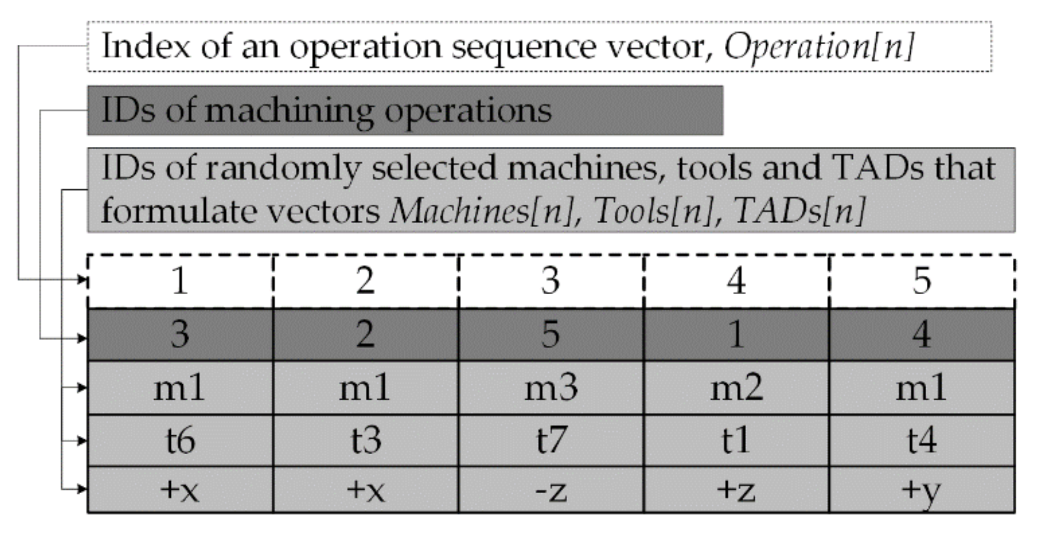
In this study, an operation sequence is represented using vectors with n bits of data. Those bits are integer values where each value contains relevant manufacturing information. Seeing that the optimization task considers the simultaneous sequencing of operations and selection of machining resources, four vectors are used to illustrate a single process plan. Figure 1 shows a simple example of a represented process plan with a total of 5 machining operations indexed from 1 to 5 (the first row). An operation sequence vector is marked with darker color and consists of bit numbers named Operation[n]. For example, Operation[3] considers the operation number 5. Under the same index, there are machine m3, tool t3 and TAD –z. These candidates are elements of the machine vector Machines[n], the tool vector Tools[n] and the TADs vector TADs[n] respectively and are visualized in a light grey color.

Since the MATLAB programming environment was selected for the implementation of the proposed GCSA approach, therefore, we will place emphasis on the types of data considered when dealing with the operation sequencing problem. All variables with their data types are shown in

Table 1. Data types of the operation sequencing variables.

Data Types	Variables	Description
double	Operation[n]	The ID of the operation as a part of an operation sequence
double	Machines[n]	The ID of the machine as a part of a machine vector of n machines for performing n operations
double	Tools[n]	The ID of the tool as a part of a tool vector of n tools for performing n operations
double	TADs[n]	The ID of the cutting tool as a part of a TAD vector of n TADs for performing n operations
cell	Machines{n}	Array of machine candidates list for n cells with each cell containing alternative machines for the n-th operation
cell	TADs{n}	Array of tool candidates list for n cells where each cell contains alternative tools for the n-th operation
cell	Tools{n}	Array of TAD candidates list for n cells where each cell contains alternative TADs for the n-th operation

.

Precedence Constraints

The precedence constraints within operation sequencing are formulated according to relevant geometrical and manufacturing considerations. They indicate the precedence relationships between operations required to generate a feasible machining sequence. Hu et al. [16] classified constraint relationships into the precedence and the clustering constraints. The precedence constraints are obligatory conditions that must be met, while on the other side, the clustering constraints do not need to be met but have effect on machining efficiency and quality. The precedence constraints can be classified into eight types: datum relationships, primary and secondary relationships, face and hole relationships, processing stage relationships, feature priority relationships, thin-wall relationships, fixed order of operations relationships and material-removal relationships. Li et al. [20] made similar classification on hard and soft constraints, where hard constraints represent obligatory conditions, while soft constraints can be violated if necessary.

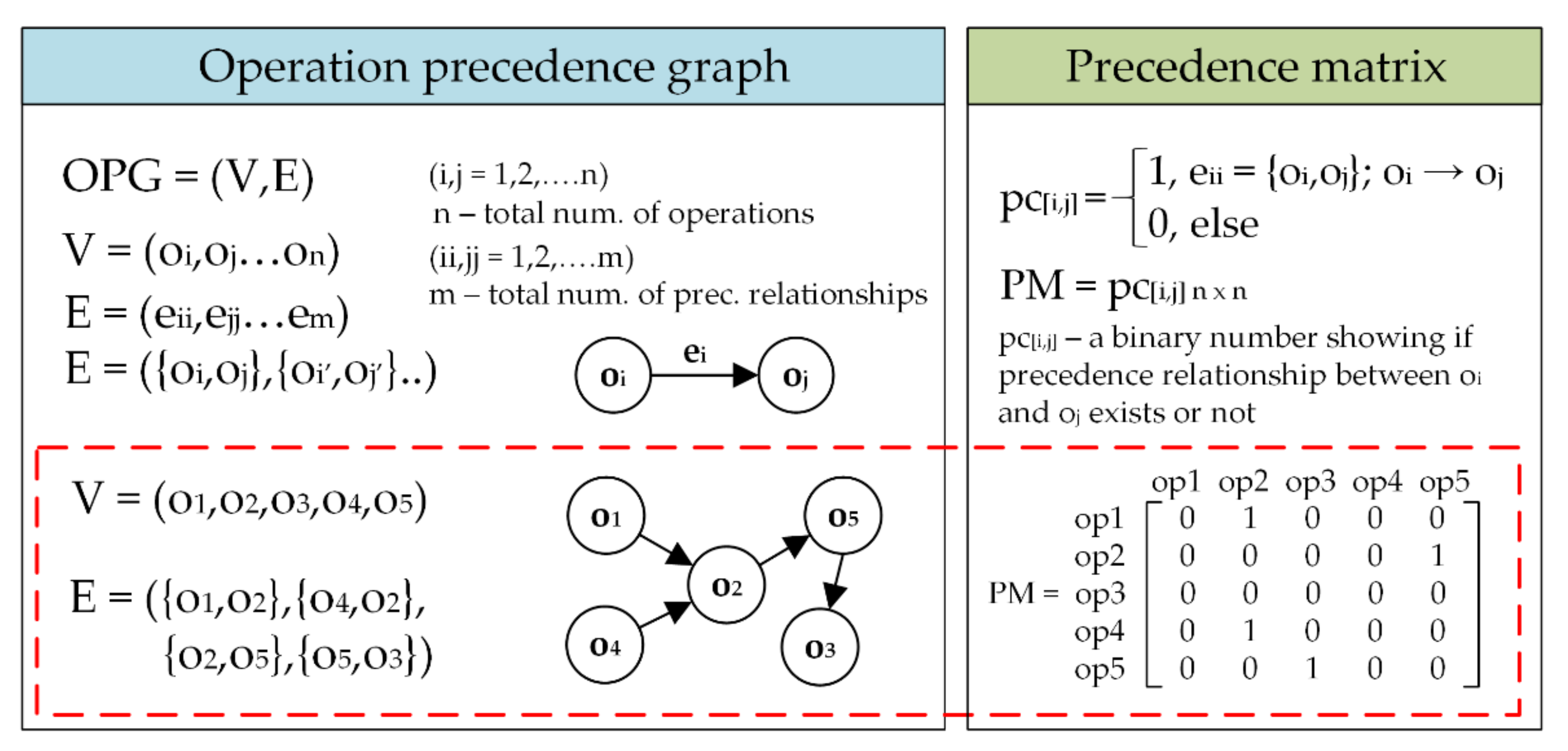
To visualize precedence relationships between operations, we adopted an operation precedence graph model (OPG). The OPG is a directed graph consisting of vertices and edges, OPG = (V, E), where vertices V represent the set of operations, while edges E denote the set of links between operation vertices. Each operation element within the operation vector is mapped to the corresponding vertex of the OPG. On the other hand, each precedence relationship is visualized using edges. Vertices that are not linked with edges have no precedence relationships between them. For easier manipulation of the data concerning precedence relationships, adjacency or precedence matrix has been adopted. Figure 2 shows the main elements of OPGs and their mapping to a matrix form. Using a simple example with five operations and four precedence constraints a precedence matrix PM is designed. The value pc[i,j] is a binary value which represents whether operation i precedes operation j or not. As shown, number 1 denotes that there is a precedence relationship between observed operations while 0 shows the lack of any precedences, i.e., no edge between operation i and operation j. By following the edges of an OPG, all the vertices should be traversed in order to obtain a feasible operation sequence.

4. A Genetic Crow Search Algorithm (GCSA) for Optimization of Operation Sequencing

4.1. Crow Search Algorithm

Crow search algorithm (CSA) was introduced in 2016 by Askarzadeh [21]. Its inspiration is derived from the crows’ intelligent behavior exhibited in their ability to hide food and use memory to recall and restore the food when necessary.

Generally, crows are considered as one of the most intelligent living organisms on the planet, with many distinctive attributes such as self-awareness, sophisticated communication, face remembrance, food hiding, memorization, thievery, thievery avoidance and so on.

Their well-known greediness and cleverness is particularly demonstrated in situations when they observe other crow’s movement with the purpose of finding better source of food and steal it once they are gone. Afterwards, crow thieves make sure they hide the stolen food and therefore avoid being victims of thievery as the previous owners. Another important element of cleverness is reflected in the fact that a crow can find out when the other crow is following it. Then, the crow that is being followed can fool the other crow by changing the direction of their flight.

From a computational point of view, the CSA algorithm is a population-based optimization algorithm which utilizes some of the exhibited crow’s intelligence. A flock of crows may consider a population of search agents N where each crow i has its position $x_i^{it}$ at iteration it. Every crow in a flock can memorize its hiding place whose position can be denoted as $m_i^{it}$. Similar to the personal best position (local best) of each particle in the PSO algorithm, the CSA considers the memory $M_i^{it}$ the best food source (hiding place) the crow i found so far. Flying around the search space and moving towards another crow’s hiding place helps crows to update their position and memory and possibly find a better food source. Two important states are possible when crow i tries to steal hidden food of crow j:

State 1: Crow j is not aware that is followed by crow i, resulting in the situation when crow i successfully commits thievery by moving towards the hiding place of crow j using the following expression:

$$X_i^{\mathit{it}+1}=X_i^{\mathit{it}}+{\mathit{rand}}_i\times \mathit{fl}\times \left(M_j^{\mathit{it}}-M_i^{\mathit{it}}\right)$$

(1)

where $X_i^{it}$. and $X_i^{it+1}$ are positions of the crow i in iterations it and it + 1 respectively, $ran{d}_i$ stands for a random number between 0 and 1, $fl$ is flight length of crow and $M_i^{it}$ and $M_i^{ij}$ are memorized positions of crow i and crow j respectively.

State 2: Crow j realizes that it is followed by crow i and fools crow i by choosing a new position randomly in order to save its food:

$$X_i^{\mathit{it}+1}=\left\{\begin{array}{c}{X}_i^{\mathit{it}+1}=X_i^{\mathit{it}}+{\mathit{rand}}_i\times \mathit{fl}\times \left(M_j^{\mathit{it}}-M_i^{\mathit{it}}\right) \mathit{if} {\mathit{rand}}_j\ge AP\\ a \mathrm{random} \mathrm{position} \mathrm{otherwise}\end{array}\right.$$

(2)

where $ran{d}_j$ denotes a random number in range [0,1] and AP is awareness probability.

Two most important parameters of the flight length and the awareness probability. The role of the flight length parameter $fl$ is to achieve equilibrium between local and the global search. Small values direct the search towards the local optimum (close to $X_i^{it}$) and large values prone towards the global optimum (away from $X_i^{it}).$ Awareness probability AP also has the similar role in balancing intensification and diversification. Just as for the flight length, small values of $AP$ increase local search capacity, and evidently, larger values emphasize global search capacity.

4.2. GCSA Methodology

The traditional CSA has been implemented mostly on continuous optimization problems with a small number of research studies done on their application in combinatorial optimization. Huang et al. [22] proposed a hybrid HCSA approach to solve the NP hard permutation flow shop scheduling problem (PFSP). They used several techniques to minimize the makespan of the PFSP, such as the smallest position value (SVP) rules to convert continuous to discrete values or job numbers, Nawaz-Enscore-Ham technique to generate a population of quality individuals and simulated annealing and variable neighborhood search algorithms to maintain the diversity of solution throughout the search process. Laabadi et al. [23] used the binary CSA to solve the two-dimensional bin packaging problem, which is also an NP-hard combinatorial problem. This approach utilizes a sigmoid function for mapping real-valued solution into binary ones and specific knowledge repair operator to improve diversity and restore feasibility of infeasible solutions.

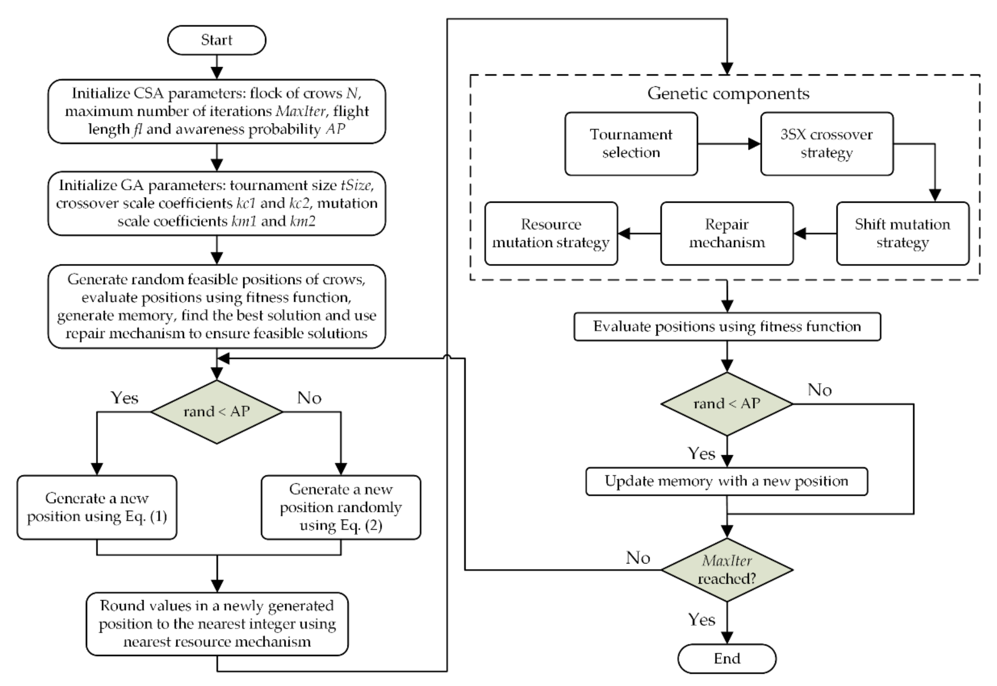
The issues of the CSA are mostly expressed by low convergence rate and entrapment in the local optima, as reported in Shirke and Udayakumar [24]. Fine tuning of the algorithm and modifications performed by various authors significantly boosted the performances of the CSA. In our study, we attempt to improve the traditional CSA in order to solve the NP hard process planning optimization problem. Therefore, we introduce a hybridized approach based on the CSA and the main components of the GA. Moreover, adaptive probability coefficients for scaling crossover and mutation operators are included to achieve the trade-off between exploration and exploitation, Dou et al. [4]. The steps of the GCSA approach are depicted on the flowchart in Figure 3.

After initializing the starting parameters of both CSA and GA, the next step is to generate population of feasible individuals using vector-based representation that presents operation sequence, machine, tool and TAD vectors as components of a single process plan. Vectors representing positions of crows in a search space are then evaluated using fitness function described in Section 4.3. They are memorized as the best local solutions found so far by each crow, after which the best solution in the flock is stored. The main loop of the GCSA starts with the standard CSA steps described by Equations (1) and (2). After these steps, the nearest resource mechanism is employed to round the resulting vector elements to the nearest integers, according to the available machine, tool and TAD candidates. The process continues with the genetic strategies which are utilized to improve diversification of search process. Here, we adopted tournament selection, 3SX crossover operator and two mutation operators, shift and resource mutation. Repair mechanism is required after the initialization stage and shift mutation to ensure feasibility of crow individuals. Then, the GCSA steps continue with the evaluation of objective function and the update of crow’s memory and the best solution (global). The search finishes after a predefined number of iterations. In the following sections, some steps are expressed in a more detailed manner.

4.3. Evaluation Criterion of the Operation Sequencing Problem

Numerous studies conducted to this day have taken into account two most common evaluation criteria for operation sequencing, manufacturing (production) time and cost. According to [6,8], detailed information about tool paths and machining parameters is not available and therefore it is not possible to accurately determine the machining cost and machining time. Hence, the total cost of production is adopted as the optimization criterion in this research. The total production cost with weight coefficients consists of the five cost factors:

(1)

Total machine cost (TMC) — the total sum of costs of used machines where machine cost indices denote the constant cost values for each machine.

(2)

Total tool cost (TTC) — the total sum of costs of used cutting tools, where tool cost indices denote the constant cost values for each tool.

(3)

Total machine change cost (TMCC)—the product of the number of machine changes and machine change cost indices, which denote the cost values of machine replacement.

(4)

Total tool change cost (TTCC)—the product of the number of tool changes and tool change cost indices, which denote the constant cost values of tool replacement.

(5)

Total setup cost (TSC)—the product of the number of setup changes and setup change cost indices which denote the constant cost values of a single machine setup.

The full description of all cost factors can be found in [4,5,6,7,8,11,14]. The total weighted production cost (TWPC) finally represents the sum of these five cost factors:

$$\mathit{T}\mathit{W}\mathit{P}\mathit{C} = w_1·TMC+w_2·TTC+w_3·TMCC+ w_4·TTCC+w_5· TSC$$

(3)

where w₁–w₅ are the corresponding weight coefficients of cost factors.

4.4. Nearest Resource Mechanism

After the main CSA steps in the GCSA approach, the values in position vectors of crow individuals are not positive integers and the next step is to convert the real values obtained by the CSA to the closest number that matches an appropriate machine, tool or TAD candidate from the set. Here, we present the nearest resource mechanism to perform the round-off procedure and assure the newly generated positions are ready for the next stage. Besides the machine and the tool vectors, the TAD position vector is represented using integer values that match the appropriate directions which are denoted as letters with negative or positive signs. In Algorithm 1 below, we show the pseudocode of the most important steps of the nearest resource mechanism. The mechanism in this example is applied to machine vector, although the principle is the same for tool and TAD vectors.

Algorithm 1. The nearest machine mechanism

Machines{} – set of all machine candidates for each operation currentMachine – current machine candidate currentOperation – current operation in a process plan diff = |Machines{currentOperation} – currentMachine| for i = 1: number of operations    if currentMachine > Machines{ currentOperation }       for j = 1: diff          check if the set Machines{currentOperation} contains          |currentMachine – diff (j)|             Use |currentMachine – diff (j)| as a machine candidate;          else             continue loop;          end if       end for    elseif currentMachine < Machines{ currentOperation }       for j = 1: diff          check if the set Machines{currentOperation} contains          |currentMachine + diff (j)|             Use |currentMachine + diff (j)| as a machine candidate;          else             continue loop;          end if       end for    else       for j = 1: diff          check if the set Machines{currentOperation} contains          |currentMachine - diff (j)|             Use |currentMachine - diff (j)| as a machine candidate;          elseif the set Machines{currentOperation} contains          |currentMachine + diff (j)|             Use |currentMachine + diff (j)| as a machine candidate;          end if       end for    end if end for

4.5. Genetic Components of the GCSA Approach

When producing a new generation of individuals, selection, crossover and mutation represent the crucial components of genetic algorithms. By mimicking the process of natural selection, they enable a population of solutions to evolve during a certain number of generations.

The first step in this process is a selection. A tournament selection operator has been adopted in this study. A few crow individuals from the flock are randomly selected to participate in the “tournament” and the crow individual with the highest fitness value wins the “tournament” and becomes a part of a new flock that consists of the best crow individuals that had previously won the competition.

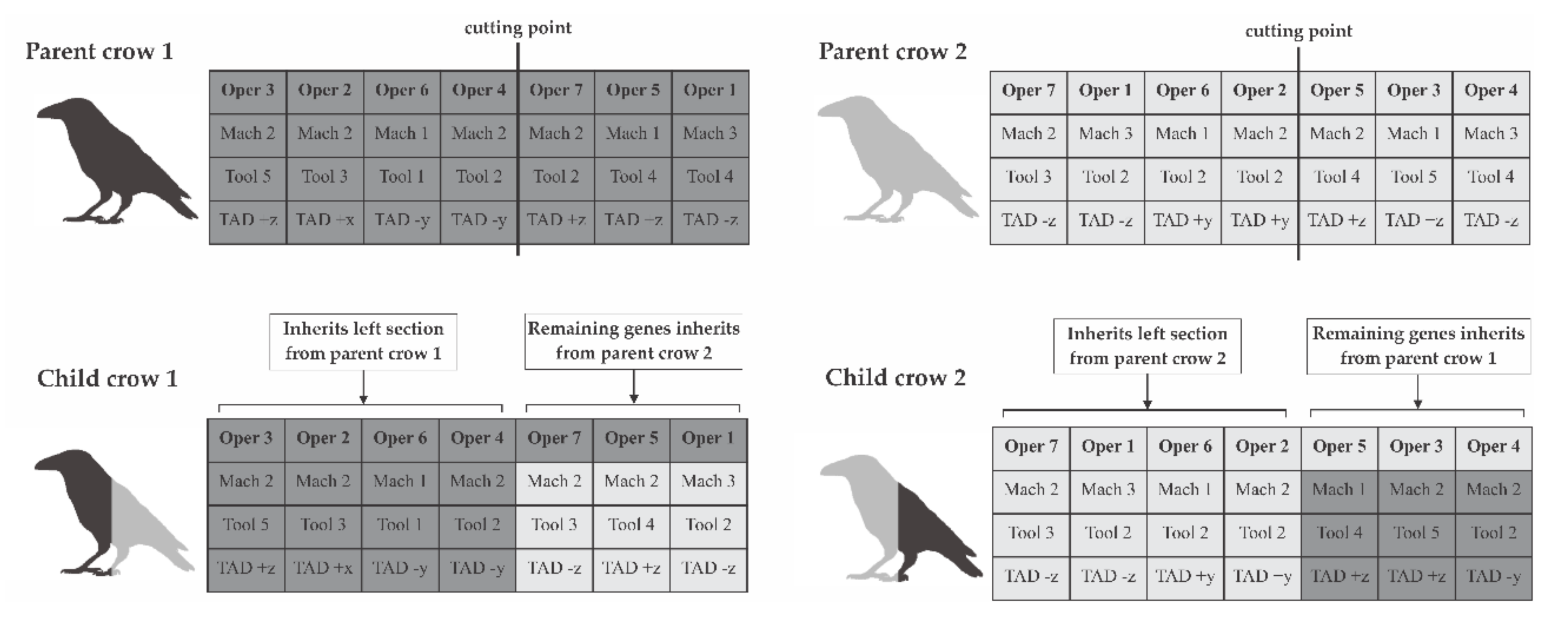
The selection step is followed by the crossover operator whose purpose is to provide information exchange between two crow individuals from a flock. In this case, the three-string crossover (3SX) proposed by Falih and Shammari [5] was adopted. The 3SX operator affects only resource vectors, e.g., machine, tool and TAD vector respectively, leaving the operation sequence vector untouched and thereby assuring the feasibility of a process plan. The following steps characterize the 3SX crossover operator:

(1)

Two crows from a new flock are randomly selected as parent crows;

(2)

From random cutting point, two parent crows are divided into sections to produce two child crows;

(3)

Resources (machines, tools and TADs) from the right section of child crow 1 are replaced by resources of the same operations from parent crow 2;

(4)

Following the same pattern, resources in the right section of child crow 2 are replaced by resources of the same operations from parent crow 1.

Figure 4 illustrates the 3SX crossover operator applied on the 7-gene length crow individual, with a random cutting point between the 4th and 5th operation index.

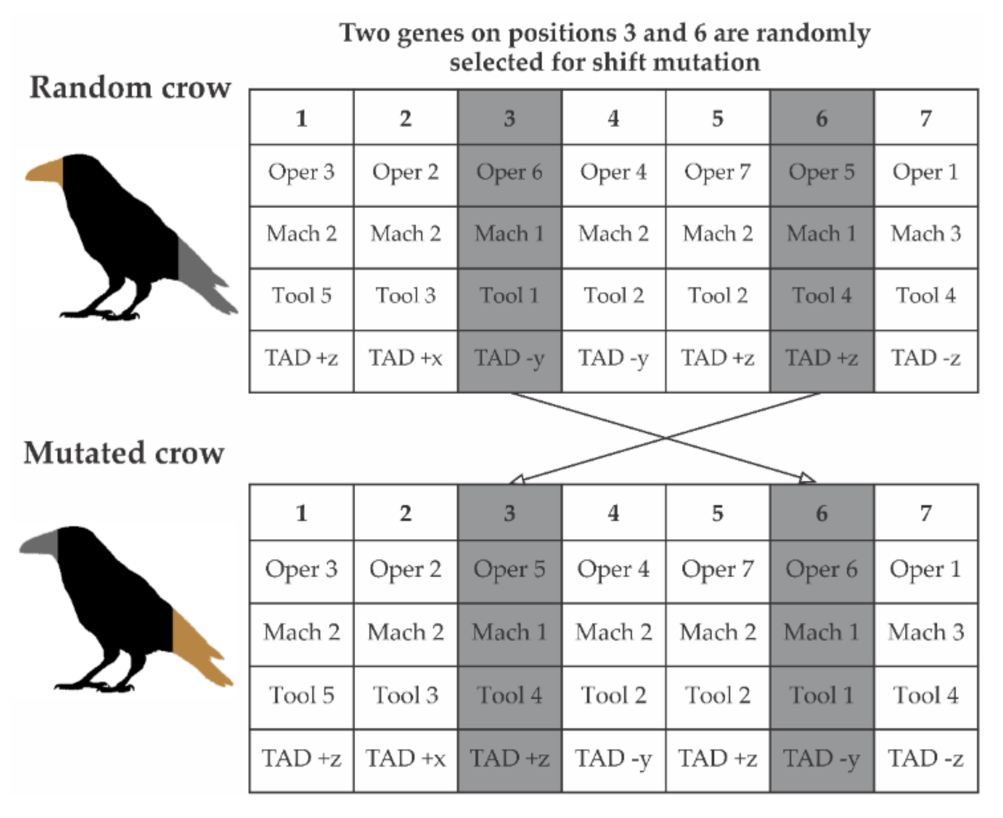
Mutation strategies bring a finishing touch to the genetic process of producing new and fitter individuals. They aim to make further improvements in diversification and avoid premature convergence of the algorithm. The first mutation operator used within the GCSA approach is the shift mutation illustrated in Figure 5. A single crow individual is randomly selected from a newly formed flock of crows and two genes (operations with its resources) are randomly selected for exchange. After exchanging the two, some of the precedence constraints may be violated, which affects the operation sequence and therefore the feasibility of a process plan. In that case, the repair mechanism has to be employed to ensure all the crows represent feasible individuals. The same mechanism is applied after the initialization stage of the GCSA. We adopted an approach similar to the constraint handling heuristic proposed by Huang et al. [11].

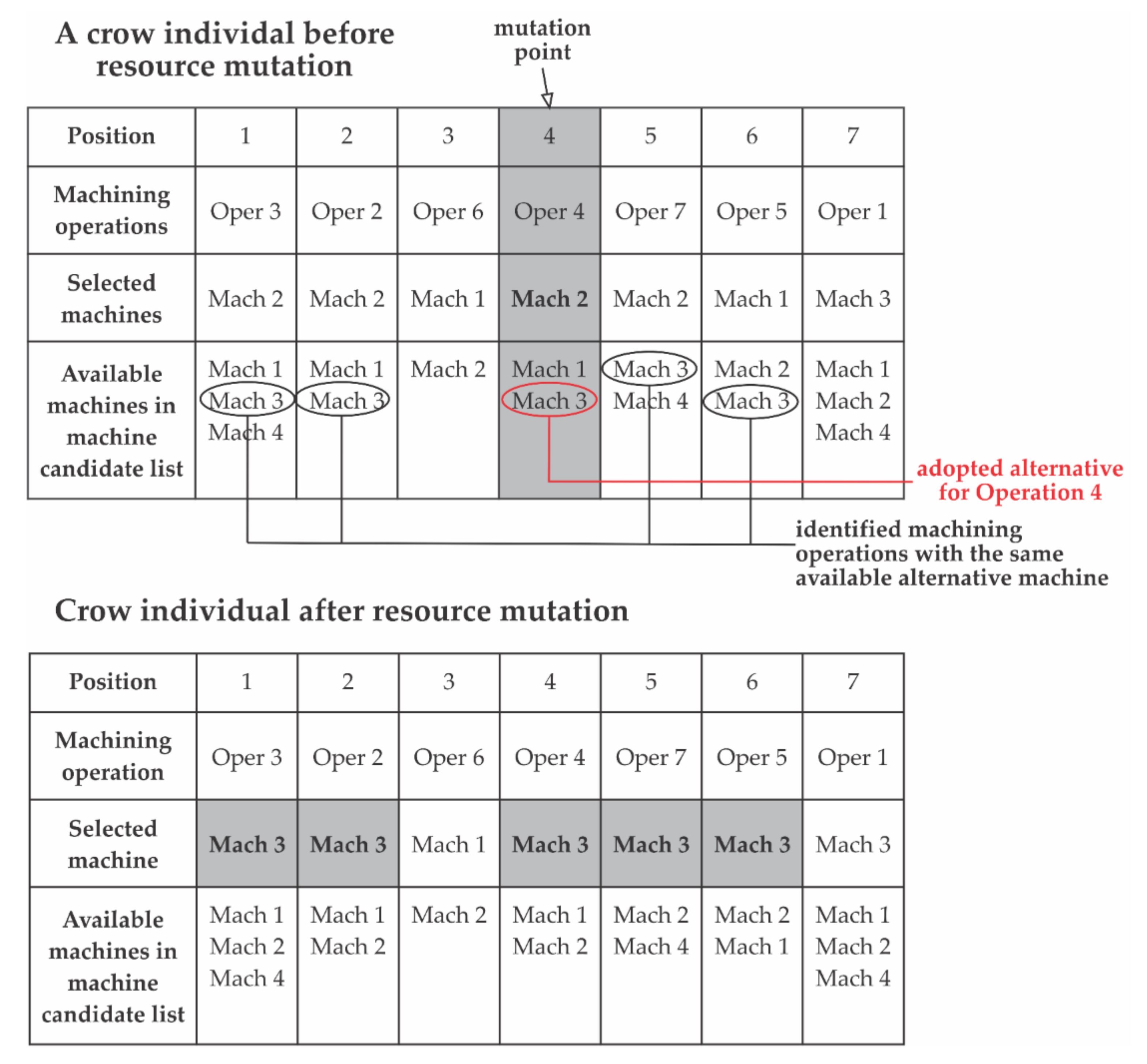
The second mutation operator is the resource mutation which, similarly to the 3SX crossover operator, operates on resource vectors, machine, tool and TAD vector respectively. The feasibility of operation sequence is therefore not questioned. The following are the steps of the resource mutation operator illustrated in Figure 6:

(1)

Randomly select a crow individual;

(2)

Randomly select the mutation point, i.e., operation with its index;

(3)

Check available machines in the Machines{} for selected operation;

(4)

Randomly select a machine from the Machines{} as the current machine;

(5)

Identify other operations that have the same machine alternative in the Machines{}.

(6)

Assign the same machine alternative as the current machine for other operations.

(7)

Repeat the same steps for tool and TAD vectors using the Tool{} and the TADs{} sets.

As reported by Dou et al. [4], fixed operators have shown to be less effective comparing to the adaptable operators, whose values vary in response to the fitness of individuals. To additionally improve search abilities of the GCSA, we included adaptive crossover and mutation probabilities:

$$p_c=k_{c1}·\frac{f_{\mathit{max}}-f_i}{·\left(f_{\mathit{max}}-f_{\mathit{avg}}\right)}+k_{c2}$$

(4)

$$p_m=k_{m1}·\frac{f_{\mathit{max}}-f_i}{·\left(f_{\mathit{max}}-f_{\mathit{avg}}\right)}+k_{m2}$$

(5)

where $f_{max}$ and $f_{avg}$ are the maximal and the average fitness value among all crow individuals in the flock, $f_i$ is the fitness of the current crow individual and $k_{c1}$, $k_{c2}$, $k_{m1}$, $k_{m2}$ are specific probability scale factors for crossover and mutation operators, respectively.

5. Case Studies

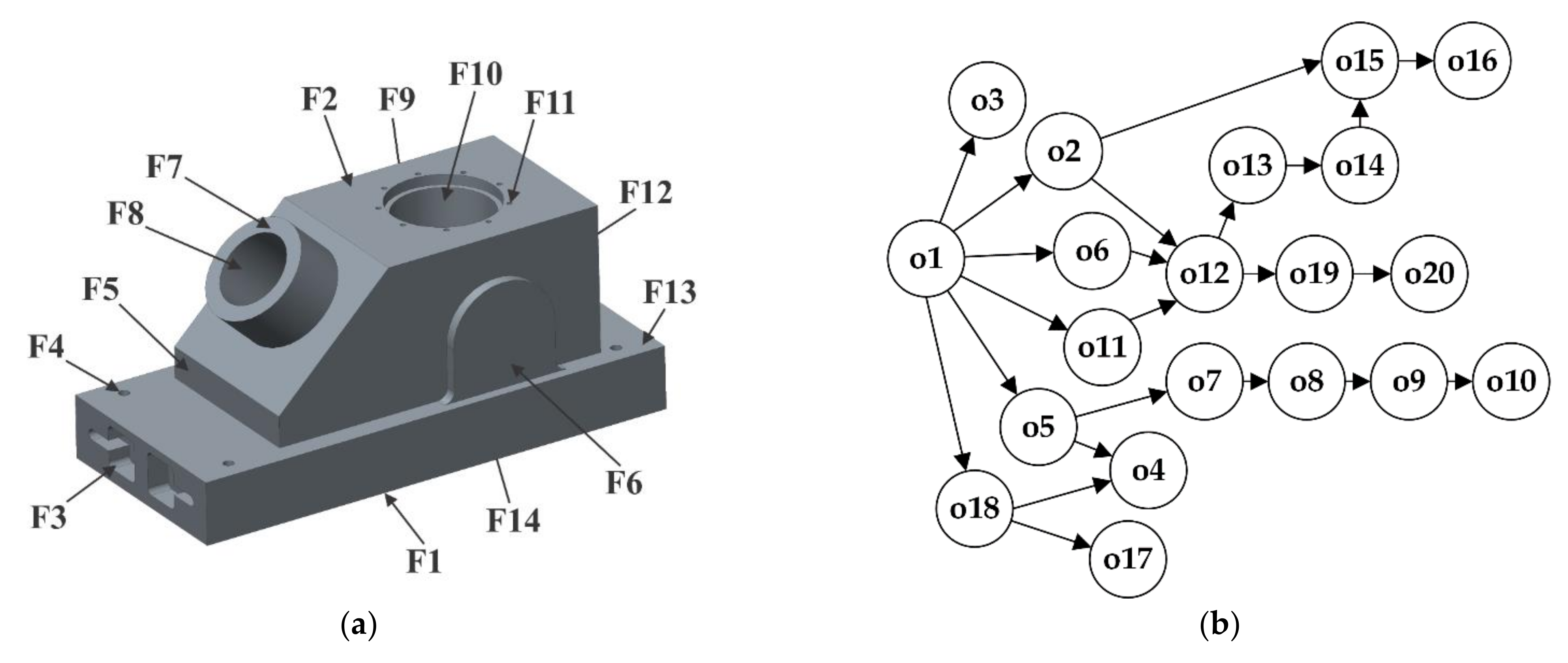
In this paper, two experimental models are used to verify the feasibility and efficiency of the proposed GCSA optimization approach, which was coded using MATLAB environment and executed on a 1.99 GHz Intel i7 processor and 8 GB RAM computer. The first case study, which represents a common test example in process planning optimization, considers the prismatic part that was initially proposed by Guo et al. [25]. It contains 14 recognized machining features and 20 selected operations. The significant manufacturing information concerning features, operations, resources as well as precedence constraints is given in

Table 2. Features, operations, resource alternatives and predecessors of Part 1.

Feature Definition	Operations	Machines{}	Tools{}	TADs{}	Predecessors
F1—A planar surface	Milling (o1)	m2,m3	t6,t7,t8	+z
F2—A planar surface	Milling (o2)	m2,m3	t6,t7,t8	-z	o1
F3—Two pockets arranged as a replicated feature	Milling (o3)	m2,m3	t6,t7,t8	+x	o1
F4—Four holes arranged as a replicated feature	Drilling (o4)	m1,m2,m3	t2	+z,-z	o1,o5,o18
F5—A step	Milling (o5)	m2,m3	t6,t7	+x,-z	o1
F6—A rib	Milling (o6)	m2,m3	t7,t8	+y,-z	o1
F7—A boss	Milling (o7)	m2,m3	t7,t8	-a	o1, o5
F8—A compound hole	Drilling (o8)	m1,m2,m3	t2,t3,t4	-a	o1, o7
	Reaming (o9)	m1,m2,m3	t9		o1, o7, o8
	Boring (o10)	m2,m3	t10		o1, o7, o8, o9
F9—A rib	Milling (o11)	m2,m3	t7,t8	-y,-z	o1
F10—A compound hole	Drilling (o12)	m1,m2,m3	t2,t3,t4	-z	o1, o2, o6, o11
	Reaming (o13)	m1,m2,m3	t9		o1, o2, o6, o11, o12
	Boring (o14)	m3,m4	t10		o1, o2, o6, o11, o12, o13
F11—Nine holes arranged as a replicated feature	Drilling (o15)Tapping (o16)	m1,m2,m3	t1	-z	o1, o2, o12, o13, o14
		m1,m2,m3	t5		o1, o2, o12, o13, o14, o15
F12—A pocket	Milling (o17)	m2,m3	t7,t8	-x	o1, o18
F13—A step	Milling (o18)	m2,m3	t6, t7	-x,-z	o1
F14—A compound hole	Reaming (o19)	m1,m2,m3	t9	+z	o1, o12
	Boring (o20)	m3,m4	t10		o1, o12, o19

. The 3D solid model with the corresponding operation precedence graph (OPG) are shown in Figure 7.

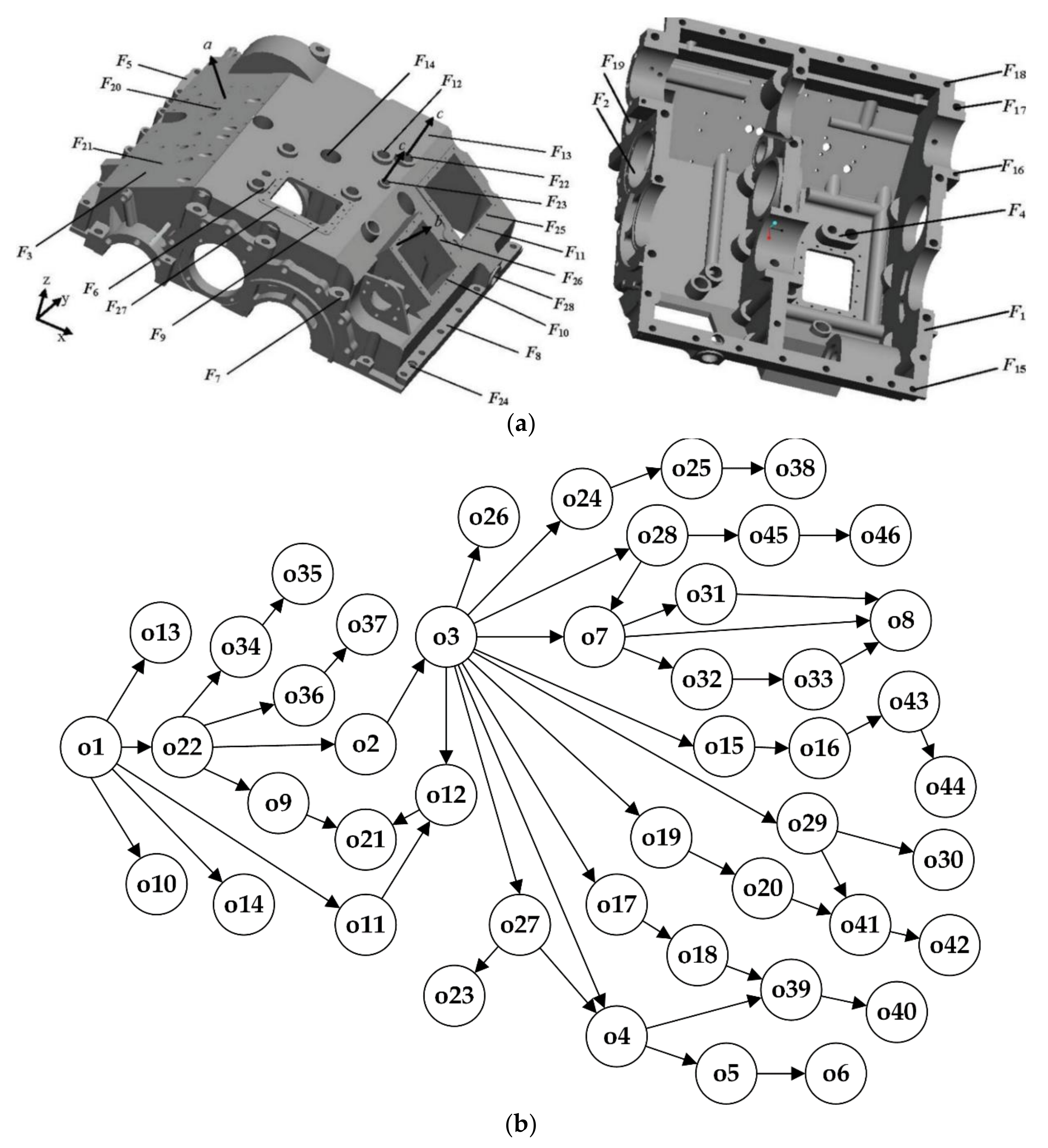
The second case study considers a complex part taken from Huang et al. [8] that consists of 28 machining features and a total of 46 machining operations. Its main manufacturing information is given in details in

Table 3. Features, operations, resource alternatives and predecessors of Part 2.

Feature Definition	Operations	Machines{}	Tools{}	TADs{}	Predecessors
F1—Flat surface	Rough turning (o1)	m1,m2	t1,t2,t3	+z
	Half-finished turning (o2)	m2	t1,t2,t3	+z	o1,o22
	Finished turning (o3)	m2	t1,t2,t3	+z	o1,o22,o2
F2—Bearing hole	Rough boring (o4)	m7, m8	t4	-y,+y	o1,o22,o2,o3,o27
	Half-finished boring (o5)	m6,m7,m8	t5	-y,+y	o1,o22,o2,o3,o27, o4
	Finished boring (o6)	m6,m7,m8	t5	-y,+y	o1,o22,o2,o3,o27, o4,o5
F3—Angular surface	Rough milling (o7)	m5,m7,m8	t7,t8,t9	-a	o1,o22,o2,o3,o27, o4
	Finished milling (o8)	m3,m4,m6	t7,t8,t9	-a	o1,o22,o2,o3,o28, o31,o32,o33
F4—Four bosses	Rough milling (o9)	m3,m4,m5	t8,t9	+z	o1,o22
F5—Plane 1	Rough milling (o10)	m3,m4,m5	t8,t9	-z	o1
F6—Top boss	Rough milling (o11)	m3,m4,m5	t8,t9	-z	o1
	Finished milling (o12)	m4,m5	t8,t9	-z	o1,o22,o2,o3,o11
F7—Six bosses	Rough milling (o13)	m3,m4,m5	t8,t9	-z	o1
F8—Plane 2	Rough milling (o14)	m3,m4,m5	t8,t9	-z	o1
F9—Top window surface	Rough milling (o15)	m3,m4,m5	t7,t8	-z	o1,o22,o2,o3
	Finished milling (o16)	m3,m4,m5	t7,t8	-z	o1,o22,o2,o3,o15
F10—Inclined plane 1	Rough milling (o17)	m3,m4,m6,m7	t7,t8	-b	o1,o22,o2,o3
	Finished milling (o18)	m3,m4,m6,m7	t7,t8	-b	o1,o22,o2,o3,o17
F11—Inclined plane 2	Rough milling (o19)	m3,m4,m6,m7	t7,t8	-b	o1,o22,o2,o3
	Finished milling (o20)	m3,m4,m6,m7	t7,t8	-b	o1,o22,o2,o3,o19
F12—The top holes	Drilling (o21)	m9,m10	t10	-z,+z	o1,o22,o2,o3,o12, o9
F13—Top plane	Rough milling (o22)	m4,m5	t7,t8,t9	-z	o1
F14—Counterbore hole	Spot facing (o23)	m9,m10	t20	-z	o1,o22,o2,o3,o27
F15—∅18H7 hole	Drilling (o24)	m9,m10	t11	+z	o1,o22,o2,o3
	Reaming (o25)	m9,m10	t22	+z	o1,o22,o2,o3,o34
F16—2-∅12.5 hole	Drilling (o26)	m9,m10	t12	+z	o1,o22,o2,o3
F17—12-∅21 hole	Drilling (o27)	m9,m10	t13	+z	o1,o22,o2,o3
F18—18-∅17 hole	Drilling (o28)	m9,m10	t14	+z	o1,o22,o2,o3
F19—Side hole	Rough boring (o29)	m7,m8	t6	-y	o1,o22,o2,o3
	Finish boring (o30)	m6,m7,m8	t6	-y	o1,o22,o2,o3,o29
F20—5-∅20 hole	Drilling (o31)	m7,m8, m9,m10	t15	-a	o1,o22,o2,o3,o7, o28
F21—24-∅8 hole	Drilling (o32)	m7,m8,m9,m10	t16	-a	o1,o22,o2,o3,o7,o28
	Tapping (o33)	m7,m8,m9,m10	t23	-a	o1,o22,o2,o3,o7, o28,o32
F22—Oil passage hole 1	Reaming (o34)	m6,m7,m8	t28	-c	o1,o22
	Tapping (o35)	m6,m7,m8	t24	-c	o1,o22,o34
F23—Oil passage hole 2	Drilling (o36)	m6,m7,m8	t17	-c	o1,o22
	Tapping (o37)	m6,m7,m8	t25	-c	o1,o22,o36
F24—∅23 Counterbore hole	Spot facing (o38)	m3,m4,m9,m10	t21	-z	o1,o22,o2,o3,o24,o25
F25—Holes in inclined plane 1	Drilling (o39)	m9,m10	t18	-b	o1,o22,o2,o3,o17, o18,o27,o4
	Tapping (o40)	m9,m10	t26	-b	o1,o22,o2,o3,o17, o18,o27,o4,o39
F26—Holes in inclined plane 2	Drilling (o41)	m9,m10	t18	-b	o1,o22,o2,o3,o29, o19,o20
	Tapping (o42)	m9,m10	t26	-b	o1,o22,o2,o3,o29, o19,o20,o41
F27—Top holes	Drilling (o43)	m3,m4,m9,m10	t18	-z	o1,o22,o2,o3,o15, o16
	Tapping (o44)	m3,m4,m9,m10	t26	-z	o1,o22,o2,o3,o15,o16,o43
F28—Oil passage hole 3	Drilling (o45)	m6,m7,m8	t19	-x	o1,o22,o2,o3,o28
	Tapping (o46)	m6,m7,m8	t27	-x	o1,o22,o2,o3,o28, o45

. The solid model of this complex part with the corresponding OPG are represented in Figure 8. The cost indices for both Part 1 and Part 2 are given in

Table 4. The cost indices of Part 1 and Part 2.

Part 1				Part 2
Cost per use
M	MC	T	TC	M	MC	T	TC	T	TC
m1	10	t1	7	m1	25	t1	5	t15	4
m2	40	t2	5	m2	45	t2	6	t16	3
m3	100	t3	3	m3	50	t3	7	t17	4
m4	60	t4	8	m4	55	t4	12	t18	2
		t5	7	m5	20	t5	13	t19	2
		t6	10	m6	80	t6	9	t20	4
		t7	15	m7	45	t7	8	t21	3
		t8	30	m8	48	t8	9	t22	5
		t9	15	m9	16	t9	10	t23	3
		t10	20	m10	18	t10	4	t24	4
						t11	4	t25	4
						t12	3	t26	3
						t13	4	t27	4
						t14	3	t28	3
Cost per change
MCCI = 160 SCCI = 100 TCCI = 20				MCCI = 120 SCCI = 90 TCCI = 15

.

5.1. Parameter Settings

In order to achieve the best possible parameter settings for the GCSA approach, we applied the Taguchi design of experiments to optimize the input parameters. The Taguchi design of experiments uses orthogonal arrays to obtain a certain number of experiments that can provide information of all factors that affect the performance of some process as expressed by Dou et al. [4]. Based on the input parameters of the GCSA and appropriate levels of variations, an experimental design matrix was formed using the standard L₃₂ Taguchi orthogonal array with 32 experimental trials. In the mentioned case studies at the input of the experimental design, the following GCSA parameters are varied: maximal number of iterations, flock size, awareness probability, flight length, tournament size and scale factors $k_{c1}$, $k_{c2}$, $k_{m1}$ and $k_{m2}$. Accuracy is increased by repeating every experiment 20 times. Therefore, the average result, the minimal result and the maximal result are used as the output parameters.

Since the two cases significantly differ in dimensions, we formed two different experimental designs in terms of levels of variation to optimize the GCSA parameters for both. In that sense, the adopted levels of variation of Part 1 are: maximal number of iterations [400,1000], flock size [60,120], tournament size [2,5], $k_{c1 }$[0.6, 0.9], $k_{c2 }$[0.3, 0.6], $k_{m1 }$[0.3, 0.6] and $k_{m2 }$[0.1, 0.3]. In order to reduce the number of experiments, we applied $L_{32}$ ($2^9$) orthogonal array, where 32 experiments are sufficient to make a conclusion. Full factorial design would require 8192 experiments to identify the effectiveness of parameters.

The adopted levels of variation of Part 2 are these: maximal number of iterations [1000,2000], flock size [80,100], awareness probability [0.2, 0.8], flight length [0.5, 2.5], tournament size [3, 5], k_c1 [0.6, 0.9], k_m1 [0.3, 0.7] and k_m2 [0.1, 0.3]. In this design, the same L₃₂ (2⁹) orthogonal array with 32 experiments is used.

Table 5. The optimal parameter settings of the GCSA approach.

Case Study	MaxIter	FlockSize	AP	fl	TourSize	kc1	kc2	km1	km2
Part 1	1000	100	0.8	0.7	5	0.8	0.6	0.3	0.3
Part 2	2000	80	0.8	0.5	5	0.86	0.2	0.3	0.3

shows the optimal GCSA parameter settings for two case studies after the response optimization using Taguchi experimental design and Minitab statistical tool.

5.2. Computational Results and Analysis

To verify the flexibility and feasibility of the GCSA approach, we proposed two case studies with several conditions. The obtained results for each condition are discussed and the feasibility of this algorithm is verified by performing comparisons with traditional and modern algorithms.

For Part 1 proposed by Guo et al. [25], the optimized parameter settings shown in Table 5 is adopted. Using these parameter settings, Part 1 was considered for three different conditions:

(1)

All manufacturing resources are available.

(2)

Tool costs and tool cost changes are excluded.

(3)

Same as the second with machine 2 and tool 8 not available.

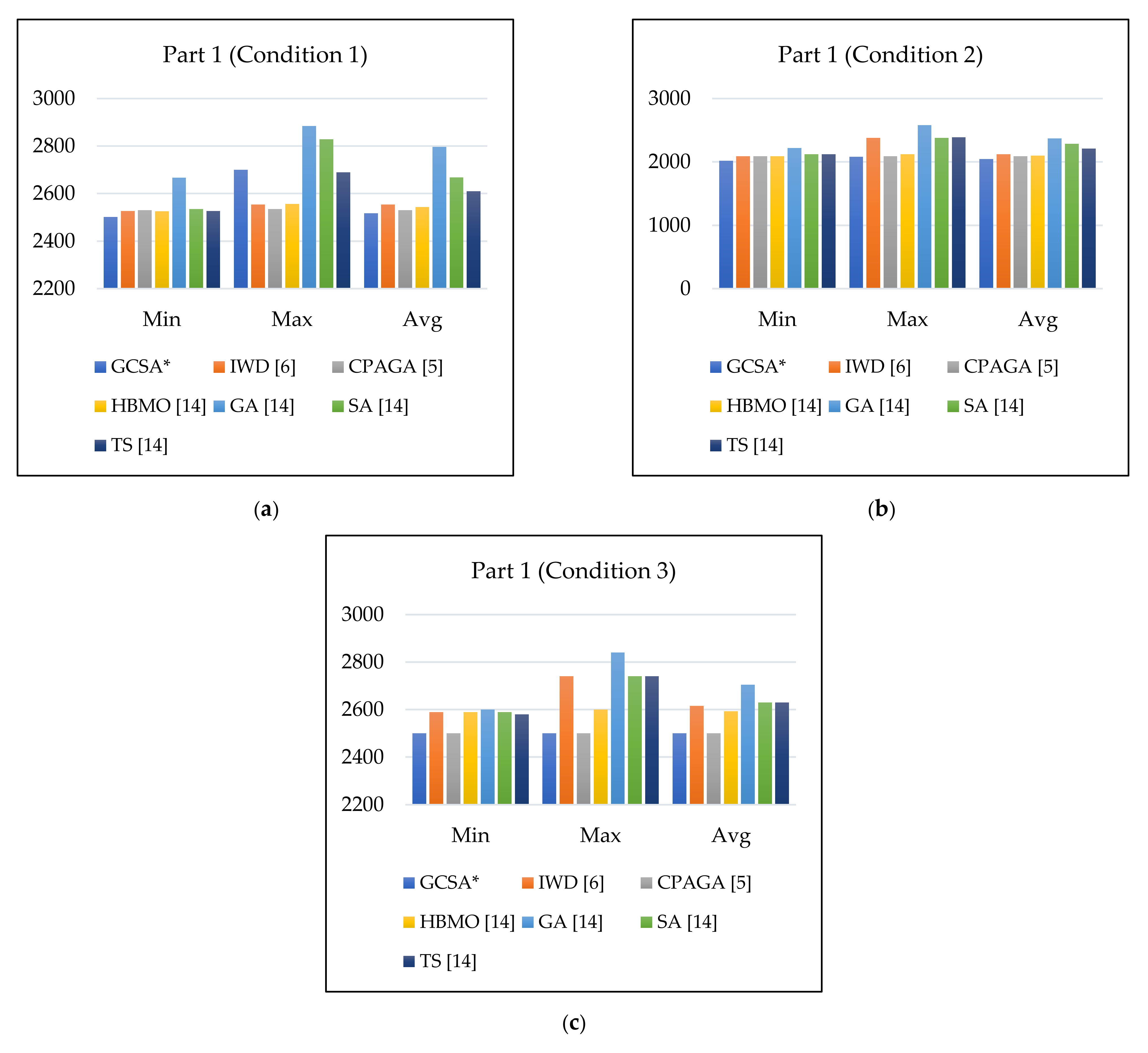
The calculation results were obtained for each of the defined conditions and the best process schemes with minimized production cost are shown in

Table 6. The best process plans for Part 1 under three different conditions.

Condition 1
Operation	1	5	3	18	2	11	6	17	4	12	13	19	7	8	9	10	20	14	15	16
Machine	2	2	2	2	2	2	2	2	2	2	2	2	2	2	2	4	4	4	1	1
Tool	6	6	6	6	6	7	7	7	2	2	9	9	7	4	9	10	10	10	1	5
TAD	+z	+x	+x	-z	-z	-z	-z	-z	-z	-z	-z	+z	-a	-a	-a	-a	+z	-z	-z	-z
TMC = 800, TMCC = 320, NMC = 2, TTC = 247, TTCC = 180, NTC = 9, TSC = 900, NSC = 9, TWPC = 2447
TMCC—Total machine change cost; NMC—Number of machine changes; TTCC—Total tool change cost; NTC—Number of tool changes; NSC—Number of setup changes
Condition 2
Operation	1	6	18	17	5	2	11	12	4	13	7	8	9	3	19	20	10	14	15	16
Machine	2	2	2	2	2	2	2	2	2	2	2	2	2	2	2	4	4	4	1	1
Tool	7	7	7	7	6	8	8	4	2	9	8	4	9	6	9	10	10	10	1	5
TAD	+z	-z	-z	-z	-z	-z	-z	-z	-z	-z	-a	-a	-a	+x	+z	+z	-a	-z	-z	-z
TMC = 800, TMCC = 320, NMC = 2, TSC = 900, NSC = 9, TWPC = 2020
Condition 3
Operation	1	3	5	7	8	9	10	2	6	11	18	12	17	13	14	15	16	4	19	20
Machine	3	3	3	3	3	3	3	3	3	3	3	3	3	3	3	3	3	3	3	3
Tool	6	6	6	7	4	9	10	6	7	7	6	4	7	9	10	1	5	2	9	10
TAD	+z	+x	+x	-a	-a	-a	-a	-z	-z	-z	-z	-z	-z	-z	-z	-z	-z	-z	+z	+z
TMC = 2000, TMCC = 0, NMC = 0, TCTC = 250, TCTCC = 3200, NCTC = 16, TSC = 500, NSC = 5, TWPC = 2500

. To present the experimental results more clearly, the comparison with results obtained by traditional and modern approaches from the literature is shown in

Table 7. The results of the GCSA compared to other algorithms for two case studies.

Part 1	Condition 1			Condition 2			Condition 3
	Min	Max	Avg	Min	Max	Avg	Min	Max	Avg
GCSA*	2502	2700	2516,9	2020	2080	2047	2500	2500	2500
IWD, Gao et al. [6]	2527	2554	2553,5	2090	2380	2123	2590	2740	2615,3
CPAGA, Falih and Shammari [5]	2530	2535	2530,5	2090	2090	2090	2500	2500	2500
HBMO, Wen et al. [14]	2525	2557	2543,5	2090	2120	2098	2590	2600	2592,4
GA, Wen et al. [14]	2667	2885	2796	2220	2580	2370	2600	2840	2705
SA, Wen et al. [14]	2535	2829	2668,5	2120	2380	2287	2590	2740	2630
TS, Wen et al. [14]	2527	2690	2609,6	2120	2390	2208	2580	2740	2630
Part 2	Condition 1			Condition 2
	Min	Max	Avg	Min	Max	Avg
GCSA*	4135	4496	4306,5	4338	4924	4544,7
CPAGA, Falih and Shammari [5]	4299	4315	4302	4503	4503	4503
GA-SA, Huang et al. [8]	4368	-	-	4450	-	-

and includes the following comparative algorithms: IWD by Gao et al. [6], CPAGA by Falih and Shammari [5], HBMO by Wen et al. [14] and GA, SA and TS results also adopted from Wen et al. [14]. The GCSA was run 20 times to verify the consistency of the obtained results. For the first condition, the minimal production cost achieved by the GCSA is 2502, which appeared 9 times. The next minimal cost is 2507 which appeared in 7 runs of the GCSA. In terms of the minimal and the average TWPC (2507 and 2516,9), according to comparative results in Table 7, it can be concluded that the GCSA outperforms other approaches, traditional and modern ones. The worst result obtained by the GCSA slightly deviates from several algorithms in this comparison. As far as the second and third conditions are concerned, the GCSA showed similar performances. For the second condition, the minimal, the maximal and the average values of the TWPC are 2020, 2080 and 2047, respectively. In comparison with other approaches, the GCSA proved its superiority regarding all three statistical parameters. For the third condition, the TWPC of 2500 appeared 20 times in 20 runs, making it the most consistent result in this study. Apart from the CPAGA, other approaches did not show similar performances. All the results from Table 7 are graphically depicted in column charts presented in Figure 9. The x-axis shows the minimal, the maximal and the average result obtained by each algorithm in the comparative study, while the y-axis shows the values of the TWPC.

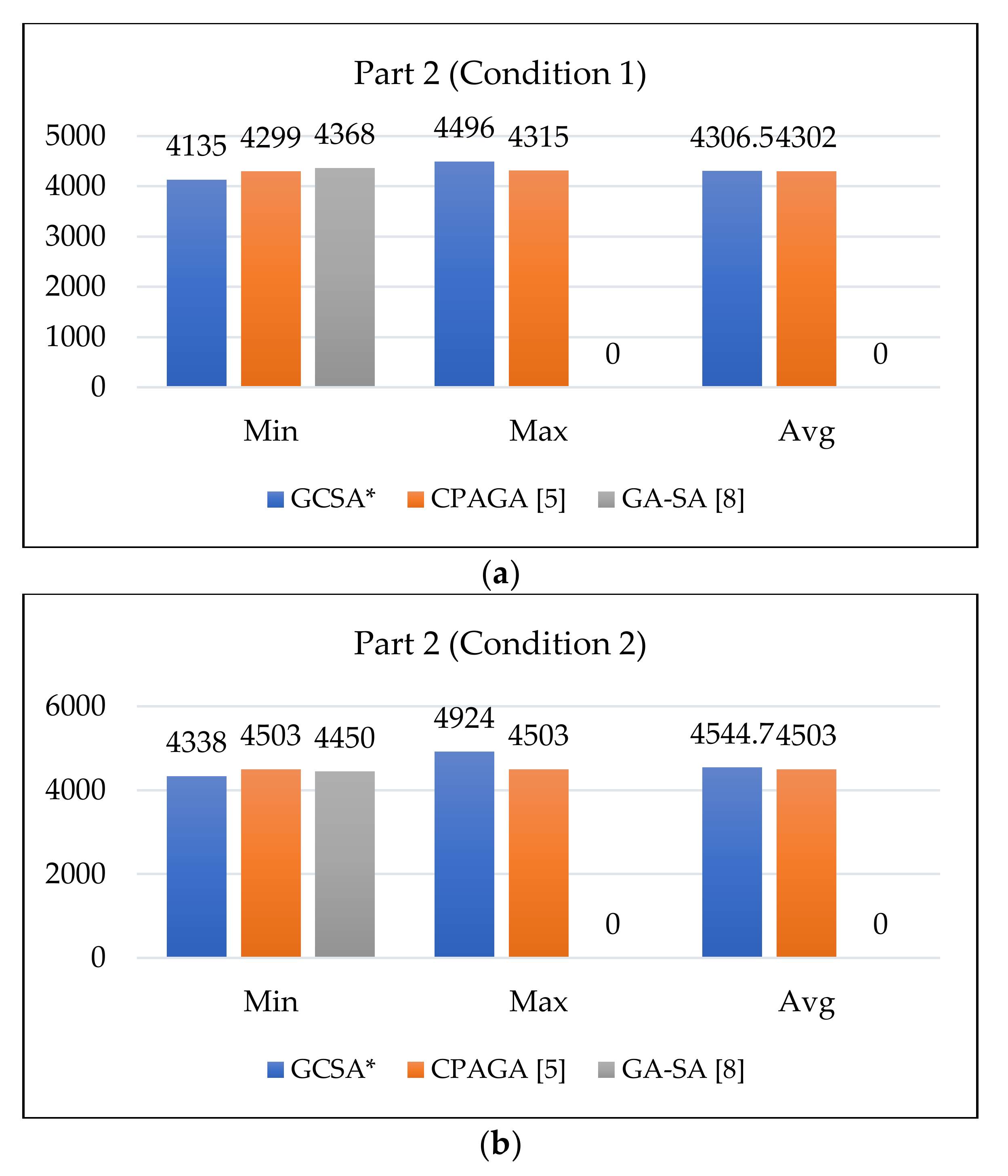
In the second study for Part 2 reported by Huang et al. [8], the optimized parameter settings also given in Table 5 are used. Since this part model has been recently proposed in scientific community, only two relevant approaches tested on this model can be adopted. The comparative results between the GCA with the CPAGA by Falih and Shammari [5] and GA-SA by Huang et al. [8] are shown in Table 7. Part 2 was carried out using two conditions:

(1)

All manufacturing resources are available.

(2)

Machines 3 and 7 and tool 8 are down.

For both conditions, the results are obtained after 20 runs. Under the first condition, the minimal TWPC is 4135, along with 4136 and 4137 which were the closest to the minimum. The average result is 4306.5, while the worst result is 4496. Only twice was the obtained TWPC above 4400, while all the other results were close to the average with four process plans reaching the TWPC below 4200. The GCSA achieved more superior result in terms of the minimal TWPC compared to the CPAGA and the GA-SA, while it showed slightly lower maximal and approximately the same average result compared to the CPAGA approach. The best solution for this condition is presented in

Table 8. The best process plans for Part 2 (Condition 1).

Indices	1	2	3	4	5	6	7	8	9	10	11	12	13	14	15	16
Operation	1	22	2	3	10	11	15	16	12	14	13	17	18	19	20	9
Machine	1	5	2	2	5	5	5	5	5	5	5	5	5	5	5	5
Tool	1	7	1	1	8	8	8	8	8	8	8	8	8	8	8	8
TAD	+z	-z	+z	+z	-z	-z	-z	-z	-z	-z	-z	-b	-b	-b	-b	+z
Indices	17	18	19	20	21	22	23	24	25	26	27	28	29	30	31	32
Operation	27	24	28	26	25	45	46	36	37	34	35	7	32	33	31	4
Machine	9	9	9	9	9	7	7	7	7	7	7	7	7	7	7	7
Tool	13	11	14	12	22	19	27	17	25	28	24	8	16	23	15	4
TAD	+z	+z	+z	+z	+z	-x	-x	-c	-c	-c	-c	-a	-a	-a	-a	-y
Indices	33	34	35	36	37	38	39	40	41	42	43	44	45	46
Operation	5	6	29	30	8	41	39	40	42	23	38	43	44	21
Machine	7	7	7	7	3	9	9	9	9	9	9	9	9	9
Tool	5	5	6	6	8	18	18	26	26	20	21	18	26	10
TAD	-y	-y	-y	-y	-a	-b	-b	-b	-b	-z	-z	-z	-z	-z
TMC = 1319, TMCC = 840, NMC = 7, TTC = 281, TTCC = 435, NTC = 29, TSC = 1260, NSC = 14, TWPC = 4135

.

Under the second condition, the best, the worst and the average TWPC using the GCSA are 4338, 4924 and 4544.7, respectively. The minimal result appeared three times in 20 runs, with more than half of the obtained TWPC being less than 4600. The best process plan for this condition is given in

Table 9. The best process plans for Part 2 (Condition 2).

Indices	1	2	3	4	5	6	7	8	9	10	11	12	13	14	15	16
Operation	1	22	2	3	15	16	11	14	13	10	12	9	24	28	27	25
Machine	1	5	2	2	5	5	5	5	5	5	5	5	9	9	9	9
Tool	1	7	1	1	7	7	9	9	9	9	9	9	11	14	13	22
TAD	+z	-z	+z	+z	-z	-z	-z	-z	-z	-z	-z	+z	+z	+z	+z	+z
Indices	17	18	19	20	21	22	23	24	25	26	27	28	29	30	31	32
Operation	26	7	31	32	33	4	5	6	29	30	45	46	34	35	36	37
Machine	9	8	8	8	8	8	8	8	8	8	8	8	8	8	8	8
Tool	12	7	15	16	23	4	5	5	6	6	19	27	28	24	17	25
TAD	+z	-a	-a	-a	-a	-y	-y	-y	-y	-y	-x	-x	-c	-c	-c	-c
Indices	33	34	35	36	37	38	39	40	41	42	43	44	45	46
Operation	17	18	19	20	8	41	39	42	40	43	23	21	44	38
Machine	4	4	4	4	4	9	9	9	9	9	9	9	9	9
Tool	7	7	7	7	7	18	18	26	26	18	20	10	26	21
TAD	-b	-b	-b	-b	-a	-b	-b	-b	-b	-z	-z	-z	-z	-z
TMC = 1509, TMCC = 840, NMC = 7, TTC = 279, TTCC = 450, NTC = 30, TSC = 1260, NSC = 14, TWPC = 4338

. Based on the comparative results in Table 7, a similar conclusion can be made as for the first condition. The GCSA overcome the results of the CPAGA and GA-SA in terms of the minimal TWPC. A smaller and larger deviation was shown in terms of the average and the maximal value, respectively. The graphical representation of the comparison with the two observed approaches is given in Figure 10.

6. Conclusions

This paper proposed a genetic crow search algorithm (GCSA) approach to deal with the operation sequencing problem in computer-aided process planning. The traditional CSA algorithm was improved using genetic components of the GA, such as tournament selection, three-string crossover, shift mutation and resource mutation strategies which were employed to balance exploration and exploitation capabilities of the GCSA. Adaptive crossover and mutation probability coefficients were also added for that purpose. The OPG graphs were introduced to represent precedence relationships among operations within a sequence, and the vector representation was adopted to manipulate the data in Matlab programming environment. The nearest resource mechanism was proposed to apply the round-off procedure after the main CSA steps. In order to assure the feasibility of crow individuals, the repair mechanism was employed after the initialization stage and after the shift mutation. In the experimental stage, two dimensionally different case studies were adopted to test the performances and flexibility of the GCSA. The adopted evaluation criterion of the operation sequencing problem was the total production cost. For several conditions, the GCSA was tested and compared with the performances of other algorithms from the literature. The comparative results are presented in tables and graphs and the GCSA showed good performances for two case studies.

As far as future work is concerned, additional modifications of the proposed GCSA approach can be made to further increase global ability of the GCSA and improve the consistency of the obtained results. Moreover, ways of including relevant information about machining parameters into operation sequencing optimization should be considered. In addition, the focus can also be on further enriching the comparative analysis by taking into consideration various other metaheuristics, hybrid algorithms and optimization methods. Finally, directions toward incorporating CSA with different heuristic mechanisms and metaheuristics other than genetic algorithms will be taken into account.

References

- Xu, X.; Wang, L.; Newman, S.T. Computer-aided process planning—A critical review of recent developments and future trends. Int. J. Comput. Integr. Manuf. 2011, 24, 1–31. [Google Scholar] [CrossRef]
- Lukić, D.; Milošević, M.; Erić, M.; Đurđev, M.; Vukman, J.; Antić, A. Improving Manufacturing Process Planning Through the Optimization of Operation Sequencing. Mach. Des. 2017, 9, 123–132. [Google Scholar] [CrossRef]
- Denkena, B.; Shpitalni, M.; Kowalski, P.; Molcho, G.; Zipori, Y. Knowledge Management in Process Planning. CIRP Ann. 2007, 56, 175–180. [Google Scholar] [CrossRef]
- Dou, J.; Li, J.; Su, C. A discrete particle swarm optimisation for operation sequencing in CAPP. Int. J. Prod. Res. 2018, 56, 3795–3814. [Google Scholar] [CrossRef]
- Falih, A.; Shammari, A.Z.M. Hybrid constrained permutation algorithm and genetic algorithm for process planning problem. J. Intell. Manuf. 2020, 31, 1079–1099. [Google Scholar] [CrossRef]
- Gao, B.; Hu, X.; Peng, Z.; Song, Y. Application of intelligent water drop algorithm in process planning optimization. Int. J. Adv. Manuf. Technol. 2020, 106, 5199–5211. [Google Scholar] [CrossRef]
- Petrović, M.; Mitić, M.; Vuković, N.; Miljković, Z. Chaotic particle swarm optimization algorithm for flexible process planning. Int. J. Adv. Manuf. Technol. 2016, 85, 2535–2555. [Google Scholar] [CrossRef]
- Huang, W.; Lin, W.; Xu, S. Application of graph theory and hybrid GA-SA for operation sequencing in a dynamic workshop environment. Comput. Aided Des. Appl. 2017, 14, 148–159. [Google Scholar] [CrossRef]
- Milošević, M.; Đurđev, M.; Lukić, D.; Antić, A.; Ungureanu, N. Intelligent Process Planning for Smart Factory and Smart Manufacturing. In Proceedings of the 5th International Conference on the Industry 4.0 Model for Advanced Manufacturing; Springer: Cham, Switzerland, 2020; pp. 205–214. [Google Scholar] [CrossRef]
- Wang, Y.F.; Zhang, Y.F.; Fuh, J.Y.H. A hybrid particle swarm based method for process planning optimisation. Int. J. Prod. Res. 2012, 50, 277–292. [Google Scholar] [CrossRef]
- Huang, W.; Hu, Y.; Cai, L. An effective hybrid graph and genetic algorithm approach to process planning optimization for prismatic parts. Int. J. Adv. Manuf. Technol. 2012, 62, 1219–1232. [Google Scholar] [CrossRef]
- Lian, K.; Zhang, C.; Shao, X.; Gao, L. Optimization of process planning with various flexibilities using an imperialist competitive algorithm. Int. J. Adv. Manuf. Technol. 2012, 59, 815–828. [Google Scholar] [CrossRef]
- Liu, X.-j.; Yi, H.; Ni, Z.-h. Application of ant colony optimization algorithm in process planning optimization. J. Intell. Manuf. 2013, 24, 1–13. [Google Scholar] [CrossRef]
- Wen, X.-y.; Li, X.-y.; Gao, L.; Sang, H.-y. Honey bees mating optimization algorithm for process planning problem. J. Intell. Manuf. 2014, 25, 459–472. [Google Scholar] [CrossRef]
- Wang, J.; Wu, X.; Fan, X. A two-stage ant colony optimization approach based on a directed graph for process planning. Int. J. Adv. Manuf. Technol. 2015, 80, 839–850. [Google Scholar] [CrossRef]
- Hu, Q.; Qiao, L.; Peng, G. An ant colony approach to operation sequencing optimization in process planning. Proc. Inst. Mech. Eng. Part B J. Eng. Manuf. 2017, 231, 470–489. [Google Scholar] [CrossRef]
- Su, Y.; Chu, X.; Chen, D.; Sun, X. A genetic algorithm for operation sequencing in CAPP using edge selection based encoding strategy. J. Intell. Manuf. 2018, 29, 313–332. [Google Scholar] [CrossRef]
- Liu, Q.; Li, X.; Gao, L. Mathematical modeling and a hybrid evolutionary algorithm for process planning. J. Intell. Manuf. 2020. [Google Scholar] [CrossRef]
- Jiang, S.; Cao, J.; Wu, H.; Yang, Y. Fairness-based Packing of Industrial IoT Data in Permissioned Blockchains. IEEE Trans. Ind. Inform. 2020, 1. [Google Scholar] [CrossRef]
- Li, W.; Ong, S.; Nee, A.Y.C. Integrated and Collaborative Product Development Environment: Technologies and Implementations; World Scientific: Singapore, 2006; Volume 2. [Google Scholar] [CrossRef]
- Askarzadeh, A. A novel metaheuristic method for solving constrained engineering optimization problems: Crow search algorithm. Comput. Struct. 2016, 169, 1–12. [Google Scholar] [CrossRef]
- Huang, K.-W.; Girsang, A.S.; Wu, Z.-X.; Chuang, Y.-W. A Hybrid Crow Search Algorithm for Solving Permutation Flow Shop Scheduling Problems. Appl. Sci. 2019, 9, 1353. [Google Scholar] [CrossRef] [Green Version]
- Laabadi, S.; Naimi, M.; Amri, H.E.; Achchab, B. A Binary Crow Search Algorithm for Solving Two-dimensional Bin Packing Problem with Fixed Orientation. Procedia Comput. Sci. 2020, 167, 809–818. [Google Scholar] [CrossRef]
- Shirke, S.; Udayakumar, R. Evaluation of Crow Search Algorithm (CSA) for Optimization in Discrete Applications. In Proceedings of the 2019 3rd International Conference on Trends in Electronics and Informatics (ICOEI), Tirunelveli, India, 23–25 April 2019; pp. 584–589. [Google Scholar] [CrossRef]
- Guo, Y.W.; Mileham, A.R.; Owen, G.W.; Li, W.D. Operation sequencing optimization using a particle swarm optimization approach. Proc. Inst. Mech. Eng. Part B J. Eng. Manuf. 2006, 220, 1945–1958. [Google Scholar] [CrossRef]
Figure 1.
Representation of an operation sequence.
Figure 2.
Operation precedence graph and precedence matrix.
Figure 3.
Flowchart of the genetic crow search algorithm (GCSA) for optimization of operation sequencing.
Figure 4.
3SX crossover operator.
Figure 5.
Shift mutation operator.
Figure 6.
Resource mutation operator.
Figure 7.
(a) Solid model and (b) the OPG of Part 1 with 20 operations.
Figure 8.
(a) Solid model and (b) the OPG of Part 1 with 46 operations.
Figure 9.
Comparison of the results under (a) condition 1, (b) condition 2 and (c) condition 3 for Part 1.
Figure 10.
Comparison of the results under (a) condition 1 and (b) condition 2 for Part 2.