Recent Developments in Experimental Techniques for Measuring Two Pulses Simultaneously

Abstract

As many high-intensity ultrafast-optical measurements involve more than one pulse—typically one to excite a medium under study and another to probe it—a technique for measuring two pulses simultaneously is highly desirable. In two decades, two-pulse measurement techniques have advanced from ambiguity-laden to a recently developed technique that can measure a pulse pair with arbitrary central wavelengths, complexities and bandwidths. Here, we review recent efforts to simultaneously measure two ultrashort laser pulses using a single device.

1. Introduction

Since their introduction several decades ago, ultrashort laser pulses have allowed researchers to make the most temporally precise and accurate measurements ever made. However, such measurements depend heavily on the ability to measure the pulses involved, and pulse-measurement techniques have traditionally lagged well behind pulse-generation techniques. This is because the measurement of an event has generally required the use of a shorter one, and ultrashort laser pulses are the shortest events ever generated. Even a self-referenced technique, that is, one that uses the event to measure itself—the best that could hope to be achieved—appeared insufficient, as the pulse is only as short as itself, not shorter. Twenty years ago, the single-pulse measurement problem was solved by the introduction of frequency-resolved optical gating (FROG), a self-referenced technique that completely measures the intensity and phase of one arbitrary ultrashort laser pulse [1,2,3]. FROG and its simplified version, GRENOUILLE [4,5,6], are widely used as self-referenced pulse measurement techniques today. In addition to the FROG family, other techniques, including multiphoton intrapulse interference phase scan (MIIPS) [7,8] and spectral-phase interferometry for direct electric-field reconstruction (SPIDER) [9,10], have also achieved common use.

In modern ultrafast optical experiments—especially high-intensity ones where nonlinear-optical processes easily generate additional pulses at new wavelengths—there is often a need to measure two independent unknown pulses simultaneously. For example, ultrafast pump-probe spectroscopy in various applications, such as material characterization and coherent control, often uses two pulses of different color and, potentially, pulse lengths, bandwidths and complexities. Its operation or temporal-resolution optimization requires measuring both the pump and probe pulses [11,12,13,14]. Also, applications involving nonlinear-optical processes, such as harmonic generation and continuum generation in optical fibers [15,16,17], which generate output pulses at different wavelengths, require complete information on both the input and output pulses to understand the underlying physics or to verify that the process has occurred properly. Therefore, a self-referenced technique that can measure two different, independent pulses simultaneously would be very useful. The technique should also have minimal restrictions on wavelengths, bandwidths and complexities. Single-shot operation would be even better, as pulses from amplified system with significant shot-to-shot fluctuations are involved.

While it is always possible to measure two pulses separately using two independent measurement devices, a single device that can measure two pulses simultaneously with minimum cost, space and complexity is desirable. Over the years, researchers have proposed different techniques to accomplish this two-pulse measurement task in a single device, such as Blind-FROG [18,19,20], complete reconstruction of attosecond bursts (CRAB) [21,22] very advanced method for phase and intensity retrieval of e-fields (VAMPIRE) [23,24] and Double Blind FROG [25,26]. Several articles have reviewed the commonly used single-pulse measurement techniques [27,28,29,30], so we will focus on the two-pulse measurement problem and review the aforementioned techniques.

2. Blind FROG and CRAB

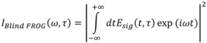
The first attempt to solve the two-pulse measurement problem in femtosecond regime is called Blind FROG. It was proposed and demonstrated by DeLong et al. in 1995 [18]. It is based on cross-correlation FROG (XFROG), which uses a known reference pulse to measure an unknown one [31]. A XFROG experimental apparatus implemented with polarization-gate (PG) geometry is shown in Figure 1. A XFROG apparatus becomes a Blind FROG when the reference pulse is an unknown pulse that also needs to be measured. Like a XFROG device, Blind FROG records one FROG trace at the camera. The mathematical expression for the recorded trace is:

(1)

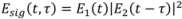
where E_sig(t) represents the signal field from the nonlinear interaction happening inside the nonlinear medium. The expression of E_sig(t) varies depending on the gating geometry in the experimental apparatus. For example, in PG geometry:

(2)

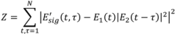
where E₁(t) and E₂(t) are the electric field of the two unknown pulses to be measured. The retrieval algorithm begins with guesses of E₁(t) and E₂(t) and generate E_sig(ω,τ) by Fourier transforming (2) with respect to t. The magnitude of E_sig(ω,τ) is replaced by the square root of the measured Blind FROG trace with the phase unchanged to generate a modified signal field, . is generated by an inverse Fourier transform. The method of generalized projections is used to generate new guesses for the fields. An error function, Z, is defined as [18]:

(3)

Figure 1. The schematic of single-shot polarization-gate (PG) cross-correlation frequency-resolved optical gating (XFROG) setup. The orange beam and red beam represent the known reference pulse and unknown pulse, respectively. The experimental apparatus is essentially a PG FROG setup with the known reference pulse replacing one of the replicas. The apparatus becomes a Blind PG FROG setup when the known reference is replaced by an unknown one.

Figure 1. The schematic of single-shot polarization-gate (PG) cross-correlation frequency-resolved optical gating (XFROG) setup. The orange beam and red beam represent the known reference pulse and unknown pulse, respectively. The experimental apparatus is essentially a PG FROG setup with the known reference pulse replacing one of the replicas. The apparatus becomes a Blind PG FROG setup when the known reference is replaced by an unknown one.

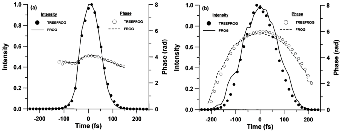
Figure 2. Electric fields of two pulses with different amount of chirp retrieved by second harmonic generation (SHG) Blind FROG (circles) compared with results retrieved by SHG FROG (lines) [18].

Figure 2. Electric fields of two pulses with different amount of chirp retrieved by second harmonic generation (SHG) Blind FROG (circles) compared with results retrieved by SHG FROG (lines) [18].

On odd iterations, the measured spectrum of pulse 2 is used to replace that of E₂, and a new guess for E₁(t) is generated by minimizing with Z respect to E₁(t). On even iterations, the operations on pulse 1 and pulse 2 reverse. The algorithm continues until the root-mean-square (rms) error between the measured and retrieved Blind FROG traces is minimized. In the original work, the Blind FROG apparatus was implemented with second harmonic generation (SHG) geometry. Figure 2 shows the two pulses with different amounts of chirp retrieved by SHG Blind FROG. The Blind FROG retrieval results were compared with measurement independently made by SHG FROG showing good agreement. However, independently measured spectra of the two pulses were also required in order to achieve convergence.

It was shown in the original Blind FROG paper that it suffers from nontrivial ambiguities, which means that multiple pulse pairs could yield Blind FROG traces that are indistinguishable, and Seifert et al. [32] later considered them in detail. As a result, Blind FROG is in general not very useful in fs-pulse characterization. However, it does find application in attosecond-pulse measurements as a result of the different physical process used to generate the signal field [21,22].

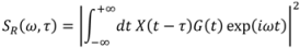
Specifically, in single-attosecond-pulse characterization, instead of using a nonlinear optical interaction to generate the signal field, a weak fs probe pulse is used to probe the phase information of the attosecond-pulse by photoionization of atoms induced by the attosecond-pulse. This technique, called complete reconstruction of attosecond bursts (CRAB), uses the idea of Blind FROG to retrieve both the fs probe pulse and attosecond pulse. In the original work, the photoelectron spectra, S(ω,τ), are measured with different delay times, τ, between the probe pulse and the attosecond-pulse. An iterative generalized-projections reconstruction method is employed to determine the electric field of the attosecond-pulse. This approach has been modified to also obtain the fs probe pulse, in effect evolving into a Blind FROG technique. The mathematical expression for the reconstructed photoelectron spectra, S_R(ω,τ), is:

(4)

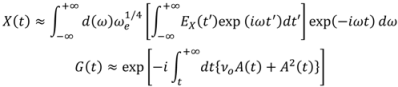
where X(t) is the reconstructed signal and G(t) is the gate. They are related (without the normalization factor) to the electric field of the attosecond-pulse, E_X(t), and the vector potential of the probe pulse, A(t), by:

(5)

where ω_e is the electron energy and v_o is a constant obtained by the reconstruction algorithm that minimizes the error between S(ω,τ) and S_R(ω,τ). The algorithm starts with setting X⁽ⁱ⁼⁰⁾(t) and G⁽ⁱ⁼⁰⁾(t) to unity, where i represents the iteration number. is generated from the X⁽ⁱ⁾(t) and G⁽ⁱ⁾(t). The intensity of is replaced by the experimentally measured S(ω,τ). New guesses for and G⁽ⁱ⁺¹⁾(t) are generated from by a generalized projections approach. The algorithm continues until the rms error between measured and reconstructed photoelectron spectra has stabilized.

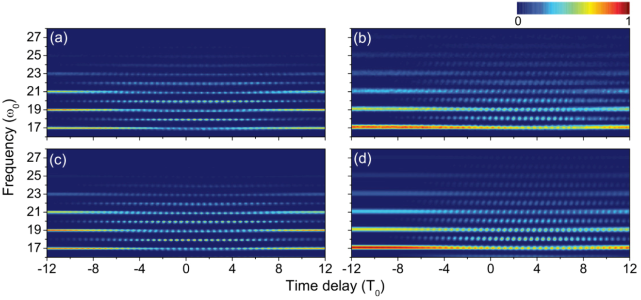
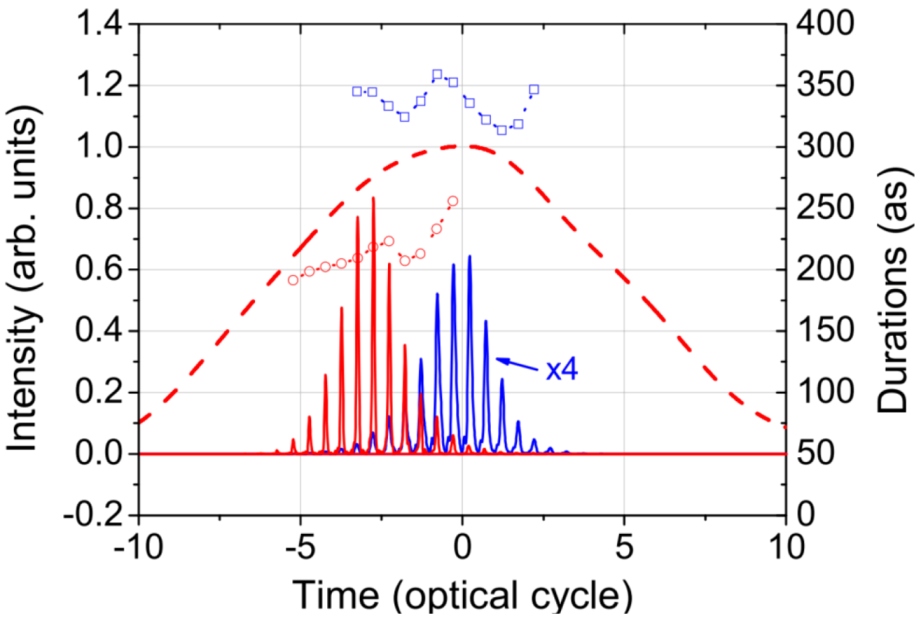
Two sets of experimental photoelectron spectra are obtained at two laser intensities, 1.6 × 10¹⁴W/cm² and 3.2 × 10¹⁴W/cm². Figure 3 shows the measured and reconstructed photoelectron spectra for a 33 fs probe pulse and attosecond-pulse trains with rms error of 0.014 and 0.012 with low- and high-intensity cases, respectively. The reconstructed temporal profiles are shown in Figure 4 which are consistent with the prediction made by numerical simulations.

Figure 3. Photoelectron spectra of He ionized by attosecond harmonic pulses with a probe laser pulse. High harmonics were obtained with a driving laser at an intensity of (a) 1.6 × 10¹⁴ W/cm² and (b) 3.2 × 10¹⁴ W/cm². The reconstructed spectra are shown in (c) and (d) for cases (a) and (b), respectively [22].

Figure 3. Photoelectron spectra of He ionized by attosecond harmonic pulses with a probe laser pulse. High harmonics were obtained with a driving laser at an intensity of (a) 1.6 × 10¹⁴ W/cm² and (b) 3.2 × 10¹⁴ W/cm². The reconstructed spectra are shown in (c) and (d) for cases (a) and (b), respectively [22].

Figure 4. Reconstructed temporal profiles of attosecond-pulse train corresponding to the cases of low (Figure 3a) and high intensities (Figure 3b), as indicated by the blue and red solid lines, respectively. The temporal profile of the reconstructed probe pulse is shown by the red dashed line. The duration of each pulse in the train is shown by squares and circles for low and high intensities, respectively [22].

Figure 4. Reconstructed temporal profiles of attosecond-pulse train corresponding to the cases of low (Figure 3a) and high intensities (Figure 3b), as indicated by the blue and red solid lines, respectively. The temporal profile of the reconstructed probe pulse is shown by the red dashed line. The duration of each pulse in the train is shown by squares and circles for low and high intensities, respectively [22].

3. VAMPIRE

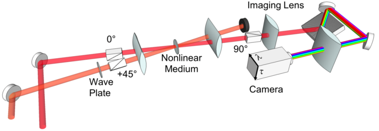
In response to the ambiguities in Blind FROG, Seifert and Stolz introduced a self-referenced two-pulse measurement technique called very advanced method for phase and intensity retrieval of e-fields (VAMPIRE) [23,24]. The technique was designed to remove the nontrivial ambiguities found in Bling FROG by generating non-centro-symmetric spectrograms. The schematic of VAMPIRE is shown in Figure 5.

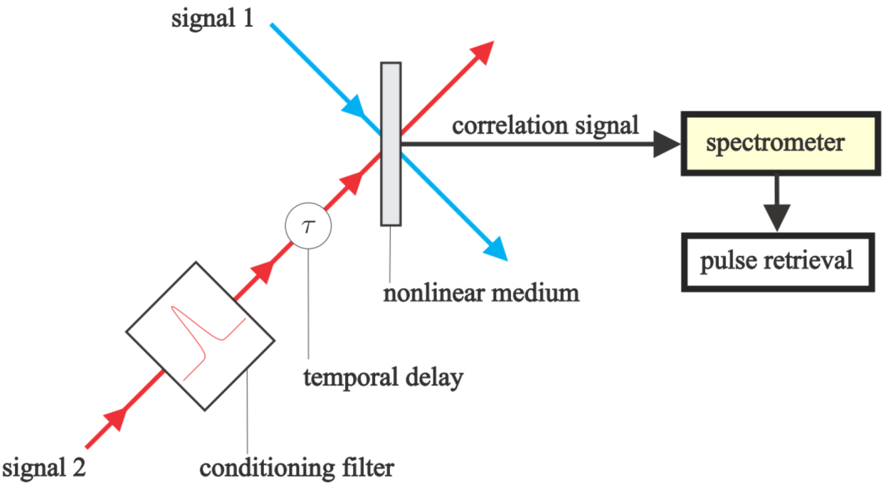
Figure 5. Optical schematic of the very advanced method for phase and intensity retrieval of e-fields (VAMPIRE) technique [24].

Figure 5. Optical schematic of the very advanced method for phase and intensity retrieval of e-fields (VAMPIRE) technique [24].

The key element of VAMPIRE is the conditioning filter, which consists of a spectral phase modulator and a temporal phase modulator. The spectral phase modulator can be implemented by an unbalanced Mach-Zehnder interferometer (MZI) with a dispersive element placed in one of the arms. The relative delay between the two replicas should not be too large to avoid sampling issues or too small to satisfy the required temporal separation. The use of the spectral phase modulator breaks the symmetry and so avoids ambiguities caused by symmetric VAMPIRE spectrograms. The relative-phase ambiguity is removed by choosing a suitable spectrum for signal 2, which covers the spectrum of signal 1. This could be done without using an external source by making a replica of signal 1 and modifying its spectrum. A temporal phase modulator, such as a self-phase modulation introduced by the Kerr nonlinearity of an optical fiber, can be used to broaden the spectrum. After the conditioning filter, the two unknown pulses interact inside a nonlinear medium to generate the cross-correlation signal. In the original work, a barium borate (BBO) crystal was used as the nonlinear medium to perform sum-frequency generation. The signal is measured by a spectrometer to generate the VAMPIRE spectrogram.

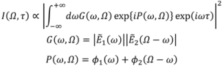
The mathematical expression for the VAMPIRE spectrogram is given by:

(6)

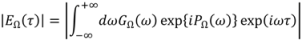
where ϕ₁ and ϕ₂ are the spectral phase of the pulses. The spectra of the pulses are measured independently and used as a constraint to the reconstruction problem, thus ϕ₁ and ϕ₂ are the unknown functions to be determined. The reconstruction algorithm starts with solving the 1D phase-retrieval problem for an arbitrary row, i.e., the arbitrary value of Ω, in the trace by using a Gerchberg-Saxton algorithm:

(7)

where |E_Ω(τ)| is given by the square root of I(Ω,τ) and G_Ω(ω) is given by the measured spectrum of the pulse. The solution of the 1D phase-retrieval problem is used as the initial guess for the neighboring row until all the rows are covered. The phase information is contained in a function, h(ω,Ω) = P(ω,Ω) + F(Ω), with P defined in Equation (6) and F being an arbitrary function. The error of each row between the measured data and the computed result is calculated. A modified function G_mod(ω,Ω) is generated by omitting rows with high error, which reduces the computational complexity in the next step. The spectral phase ϕ₁ and ϕ₂ are reconstructed by using a singular value decomposition (SVD) algorithm with G_mod and h as the input. The arbitrary function F is eliminated in the last step.

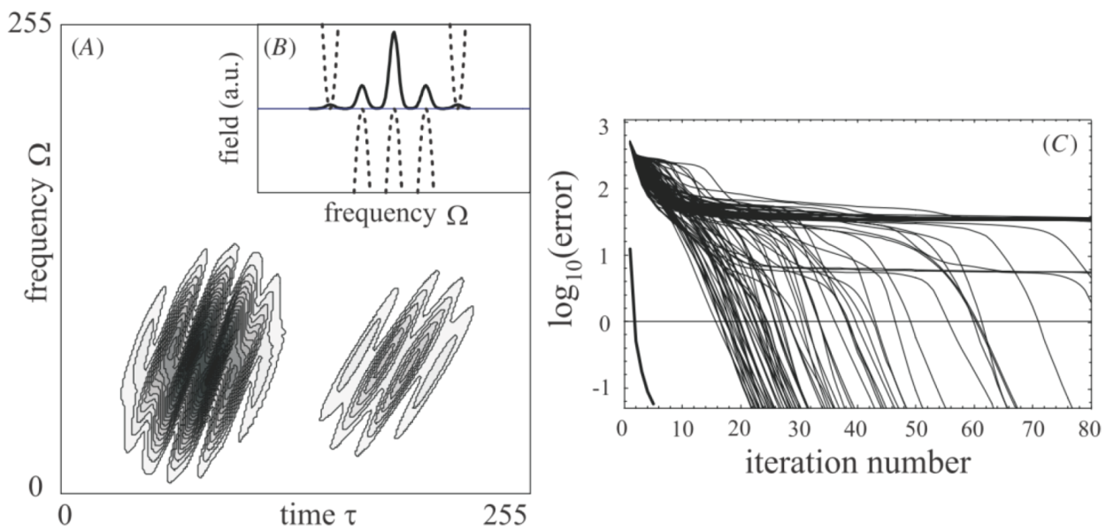
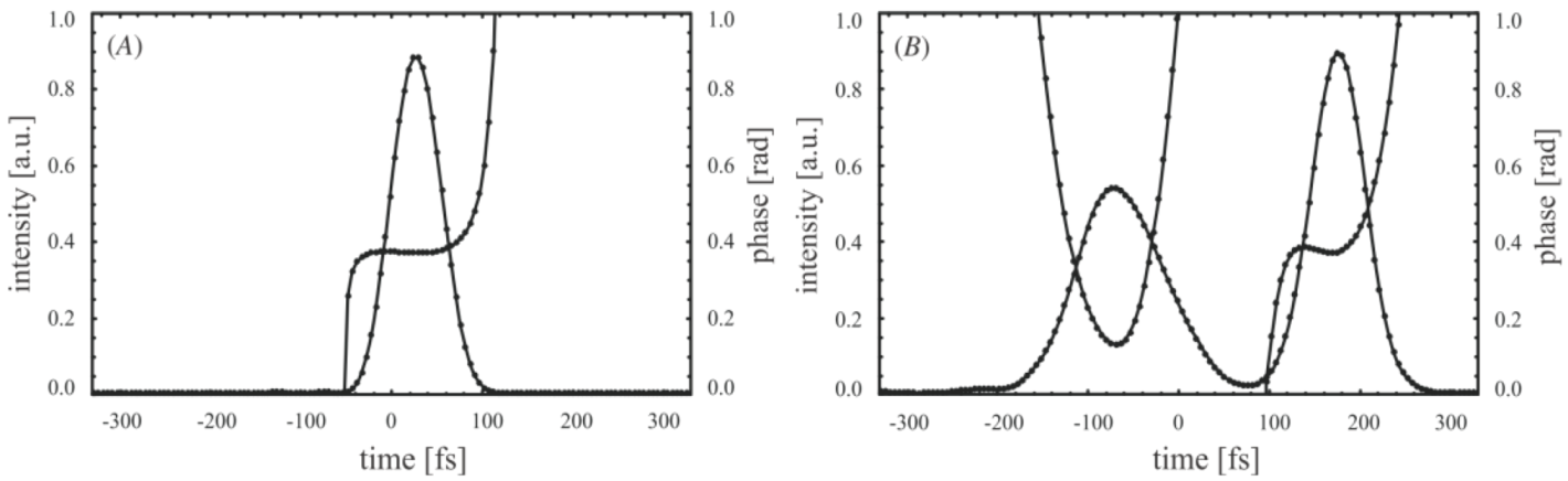
Figure 6. (A) Simulated VAMPIRE spectrogram generated with the signal in (B) and a filtered signal Gaussian. (C) Rate of convergence plots. The plots on the right side show the convergence behavior of principle component generalized projection algorithm (PCGPA) with random initial guesses, and the plot on the lower left corner shows convergence of the VAMPIRE algorithm [24].

Figure 6. (A) Simulated VAMPIRE spectrogram generated with the signal in (B) and a filtered signal Gaussian. (C) Rate of convergence plots. The plots on the right side show the convergence behavior of principle component generalized projection algorithm (PCGPA) with random initial guesses, and the plot on the lower left corner shows convergence of the VAMPIRE algorithm [24].

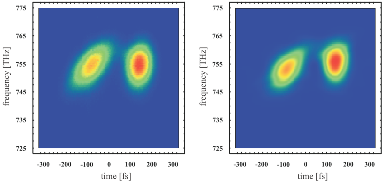
The algorithm was tested with a simulated pulse pair: a signal pulse shown in Figure 6B and a filtered single Gaussian. The convergences of the reconstruction algorithm and principle component generalized projection algorithm (PCGPA) are shown in Figure 6C. Convergence using the VAMPIRE reconstruction algorithm is reached regardless of the initial guess. Two unknown pulses are measured and reconstructed experimentally. The corresponding VAMPIRE spectrograms are shown in Figure 7 and the temporal information are shown in Figure 8. The reconstructed double pulse shows a stretch factor of 1.59 which agrees well with the theoretical prediction of 1.63.

Figure 7. The measured (left) and reconstructed (right) VAMPIRE spectrograms [24].

Figure 7. The measured (left) and reconstructed (right) VAMPIRE spectrograms [24].

Figure 8. The reconstructed signal 1 (A) and signal 2 (B) of two unknown pulses corresponding to the VAMPIRE spectrogram shown in Figure 7 [24].

Figure 8. The reconstructed signal 1 (A) and signal 2 (B) of two unknown pulses corresponding to the VAMPIRE spectrogram shown in Figure 7 [24].

4. Double Blind FROG

Recently, another two-pulse measurement technique, a variation of the original Blind FROG, was demonstrated and is called Double Blind FROG (DB FROG) [25,26]. Note the lack of a hyphen between “Double” and “Blind” in its name to avoid confusion with the medical-experiment technique in which neither the experimenter nor the patient has knowledge of the sample in question. DB FROG’s name actually implies that it is effectively two Blind FROG setups. Indeed, the experimental apparatus of DB FROG is modified from Blind FROG so that an extra FROG trace is measured. DB FROG is best implemented in PG geometry, in particular, a PG XFROG setup (see Figure 1). The only required modifications to a standard Blind FROG or XFROG apparatus are an additional analyzer oriented at −45°. Also, if desired, an additional spectrometer and camera can be used to record the extra FROG trace, although it is quite reasonable to record both traces using a single spectrometer and camera.

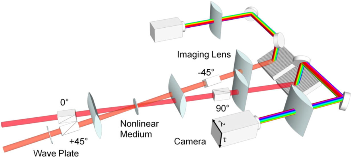
The two unknown pulses interact with each other in a χ⁽³⁾ nonlinear medium, such as a fused silica window. The polarizations of pulse 1 and pulse 2 are set to be 45° relative to each other, for example, pulse 1 at 0° and pulse 2 at 45°, as shown in Figure 9. When the two pulses with 45° relative polarization interact in a χ⁽³⁾ nonlinear medium, polarization rotation occurs due to birefringence induced via the third-order nonlinear polarization. This interaction is automatically phase-matched for any crossing-angles, wavelengths and bandwidths. Both pulses experience polarization rotation and will pass through the crossed-polarizer pair in each arm. A spectrometer and camera are placed in each beam path to record a spectrogram (FROG trace), one from each pulse, so two FROG traces are generated in one measurement.

Figure 9. The schematic of single-shot Double Blind (DB) PG FROG for measuring an unknown pulse pair [25].

Figure 9. The schematic of single-shot Double Blind (DB) PG FROG for measuring an unknown pulse pair [25].

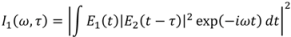
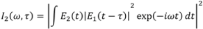
The two measured DB PG FROG traces are given by:

(8)

(9)

where I₁(ω,τ) represents trace 1, with pulse 1 and pulse 2 acting as the unknown and the known reference pulses, respectively. In trace 2, the roles of pulse 1 and 2 are reversed. Each of the DB PG FROG traces is essentially a PG XFROG trace, but with the known reference pulse replaced by an unknown pulse. In the standard generalized-projections XFROG phase-retrieval algorithm, the known reference pulse is the gate pulse, and the unknown is retrieved by using this gate pulse. DB FROG has two unknown pulses, instead of one known and one unknown pulse. The DB FROG retrieval problem consists of two linked XFROG retrieval problems: in order to retrieve one pulse correctly, the other pulse must be known, and vice versa.

The DB FROG retrieval algorithm begins with random initial guesses for both E₁(t) and E₂(t). In the first half of the cycle, the DB FROG retrieval algorithm assumes E₁(t) is the unknown pulse and E₂(t) is the gate pulse (even though a random guess is usually not close to the correct gate, it is a sufficient starting point). The algorithm retrieves pulse 1 from trace 1 as a PG XFROG problem. After the first half cycle, the retrieved pulse 1 is not the correct pulse, because pulse 2 is not the correct gate pulse to begin with, but it is a better estimate of it than the initial guess, because this estimate more closely satisfies the trace I₁(ω,τ). In the second half of the cycle, the roles of 1 and 2 are switched. Trace 2 and the improved version of E₁(t) (acting as the gate pulse) are used to retrieve E₂(t). After one complete cycle, both improved versions of E₁(t) and E₂(t) are used as the inputs for the next cycle. This process is repeated, until the two DB PG FROG traces generated from E₁(t) and E₂(t) match the experimentally measured traces, that is, the difference between the measured and retrieved traces is minimized. Standard noise-reduction and background subtraction are performed on the two measured traces before running the retrieval algorithm. The convergence of DB FROG is defined, similarly to other standard FROG techniques, by the G-error (the root-mean-square difference of the measured and retrieved traces), one for each DB PG FROG traces.

Figure 10. Simulations of DB PG FROG for two complex pulses. The two “measured” traces (a) and (c) are shown in the traces labeled “Simulation”, and their retrieved traces (b) and (d) are shown to their immediate right. The retrieved intensities and phases are shown in (e) to (h) by the solid-color lines. The actual intensity and phase of the simulated pulses are shown as dashed black lines. Both of these simulated complex pulses have time-bandwidth products of about seven, and 1% additive Poisson noise was added to the simulated traces to simulate noisy measurements [25].

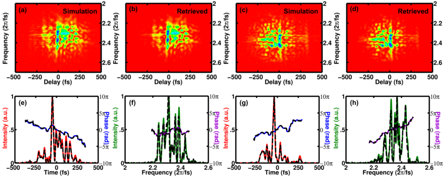
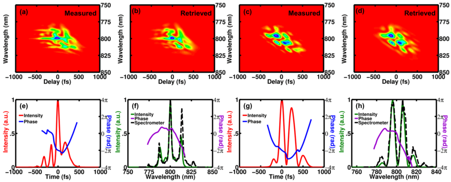
Figure 10. Simulations of DB PG FROG for two complex pulses. The two “measured” traces (a) and (c) are shown in the traces labeled “Simulation”, and their retrieved traces (b) and (d) are shown to their immediate right. The retrieved intensities and phases are shown in (e) to (h) by the solid-color lines. The actual intensity and phase of the simulated pulses are shown as dashed black lines. Both of these simulated complex pulses have time-bandwidth products of about seven, and 1% additive Poisson noise was added to the simulated traces to simulate noisy measurements [25].

The DB FROG algorithm was tested with simulated DB PG FROG traces. Complex pulses with time-bandwidth-products (TBPs) of ~7 were successfully retrieved from simulated traces, even with 1% Poisson noise added to simulate experimental conditions. Figure 10 shows one of the pulse pairs. The traces yielded 0.085% G-error, which indicated a good fit. The retrieved pulses agreed very well with the actual pulses used to generate the traces for retrieval. No nontrivial ambiguities were found in the numerical work, except for the well-known trivial ambiguities of most pulse-measurement techniques, the zeroth and first-order spectral phase.

A pair of complex pulses was used to test its measuring ability. The measured and retrieved traces are shown in Figure 11. Trace 1 measured a chirped pulse train. It was generated by an etalon and chirped by 2 cm SF11 glass block. Trace 2 measured a chirped double pulse. It was generated by a Michelson interferometer with a tunable delay arm and chirped by 4 cm of SF11 glass. Both traces yielded G-error of ~0.8%. Temporal intensity distortions were observed in both pulses, a well-known characteristic of chirped-pulse beating, as expected. Independent measurement of the spectrum made with a spectrometer for both pulses were plotted in black dashed-line. The spectral peak locations match very well between the DB PG FROG and spectrometer measurements, confirming that the retrieved pulses are indeed correct.

Figure 11. The measured trace for (a) a chirped pulse train and (c) a chirped double pulse. The retrieved trace (b) and (d) with FROG error of 0.81% and 0.74% for (a) and (c), respectively. (e) and (g), retrieved pulse intensity and phase in temporal domain showing structures from chirped pulse beating. (f) and (h), the measured spectrum and the spectral phase compared with measurement made by a spectrometer [26].

Figure 11. The measured trace for (a) a chirped pulse train and (c) a chirped double pulse. The retrieved trace (b) and (d) with FROG error of 0.81% and 0.74% for (a) and (c), respectively. (e) and (g), retrieved pulse intensity and phase in temporal domain showing structures from chirped pulse beating. (f) and (h), the measured spectrum and the spectral phase compared with measurement made by a spectrometer [26].

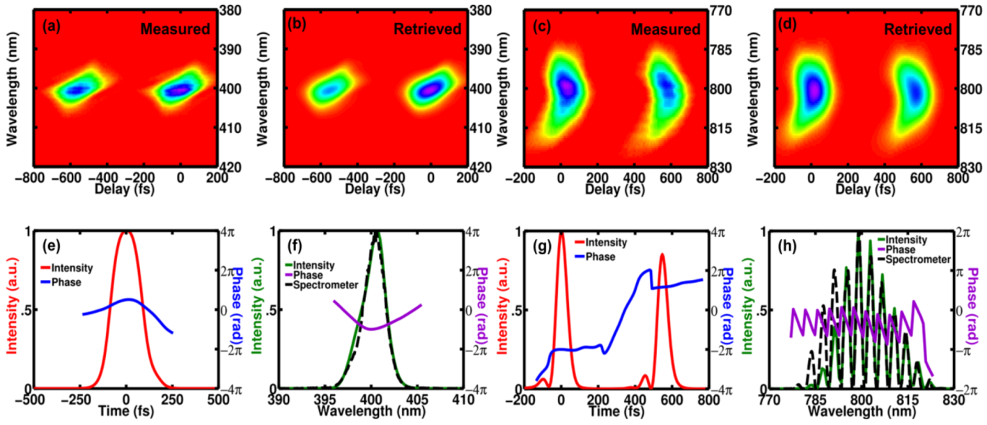
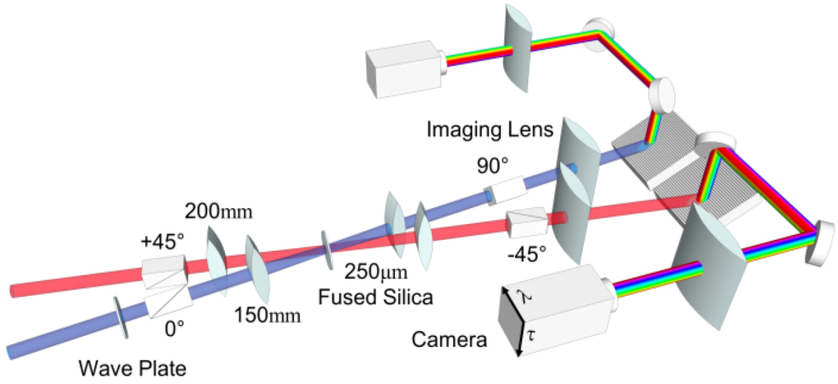
After the demonstration of DB PG FROG to measure two unknown pulses with the same center wavelength and bandwidth, it was used to measure a pair of pulses with two different center wavelengths and bandwidths. This is an important feature of DB PG FROG, which the measurement of pulses without a precise phase-matching condition. The experimental setup (shown in Figure 12) is slightly modified from the original setup such that each beam path uses a separated pair of focusing and collimating lens to avoid chromatic aberration.

The two-color measurement was made with a pair of pulses with center wavelengths of 400 nm and 800 nm (blue and red). The measured and retrieved traces are shown in Figure 13. A well-separated double pulse in red was generated by a Michelson interferometer, while the blue pulse was a simple pulse. The G-errors were 0.8% and 0.5% for the blue pulse and red pulse, respectively. The spectra of both red and blue pulses were measured independently and plotted in black dashed-lines. The spectral fringes in the red spectrum overlapped well between the measurement made by DB PG FROG and the spectrometer. The average spectral fringe separations were 3.82 nm and 3.91 nm from the spectrum measured by spectrometer and DB PG FROG, respectively. The predicted value of the temporal separation between the double pulses was 558 fs, which was calculated from the average spectral fringe separation measured by the spectrometer. The temporal peak separation retrieved by DB PG FROG was 547 fs, consistent with the prediction.

Figure 12. The schematic of single-shot DB PG FROG for measuring an unknown pulse pair at different wavelengths (400 nm and 800 nm in the actual experimental demonstration) [26].

Figure 12. The schematic of single-shot DB PG FROG for measuring an unknown pulse pair at different wavelengths (400 nm and 800 nm in the actual experimental demonstration) [26].

Figure 13. The measured DB PG FROG traces for (a) a simple pulse at 400nm and (c) a well separated double pulse at 800nm. The retrieved traces (b) and (d) with a FROG error of 0.83% and 0.52% for (a) and (c), respectively. (e) and (g), retrieved pulse intensity and phase in temporal domain. (f) and (h), the measured spectrum and the spectral phase compared with a measurement made by a spectrometer [26].

Figure 13. The measured DB PG FROG traces for (a) a simple pulse at 400nm and (c) a well separated double pulse at 800nm. The retrieved traces (b) and (d) with a FROG error of 0.83% and 0.52% for (a) and (c), respectively. (e) and (g), retrieved pulse intensity and phase in temporal domain. (f) and (h), the measured spectrum and the spectral phase compared with a measurement made by a spectrometer [26].

5. Summary

Several ultrashort pulse measurement techniques have attempted to solve the two-pulse measurement problem. The earliest attempt, Blind FROG, found limited application in characterizing fs-pulses, due to the existence of nontrivial ambiguities. The experimental apparatus and retrieval algorithm developed for Blind FROG, however, inspired other measurement techniques that can solve the two-pulse measurement problem. Based on the idea of Blind FROG, CRAB has performed simultaneous attosecond and femtosecond pulse retrieval. No nontrivial ambiguities are known in CRAB reconstruction, because the signal field generation mechanism takes a different form than that of the originally proposed sum-frequency-generation Blind FROG. The generalized projections reconstruction algorithm is robust and requires no extra information for the pulses to converge.

For pairs of unknown fs-pulses, VAMPIRE was developed to avoid the nontrivial ambiguities found in Blind FROG. It introduces a spectral phase modulator and a temporal phase modulator into the experimental apparatus in order to break the symmetry of the measured spectrogram. These additional modulators add significant extra complexity to the apparatus, but they effectively remove the nontrivial ambiguities resulting from a symmetric spectrogram. The reconstruction algorithm applies the Gerchberg-Saxton algorithm to solve rows of 1D phase retrievals, which gives a reliable way to generate the initial guess. The spectra of both pulses are measured and used as the constraint in the problem. The SVD algorithm provides a fast and robust way to reconstruct the spectral phase information of the unknown pulses. However, the requirement of using the measured spectra of the unknown pulses as constraints adds additional complication to the VAMPIRE technique.

A recently developed technique based on the original Blind FROG, called DB FROG, accomplishes the two-pulse measurement task without such constraints or complexity. It slightly modifies Blind FROG by adding an extra polarizer and an extra spectrometer to measure an extra FROG trace. The retrieval algorithm solves a pair of linked XFROG problems using a modified algorithm based on the standard XFROG one. The algorithm requires no additional information from the pulses and finds no nontrivial ambiguities, as determined from numerical simulations. If implemented in the PG geometry, there is no constraint on the spectra of the pulses, due to the unlimited phase-matching bandwidth of the nonlinear optical interaction. This implies that DB PG FROG can be used to measure pulse pairs at any central wavelengths and with any bandwidths.

Ultrashort-pulse characterization techniques allow researchers to gain more understanding of their experimental tools. These advances in two-pulse measurement now permit ever more general and arbitrary pulse pairs to be measured. And in the near future, it may even be possible, using them, to measure extremely complex pulse pairs, such as supercontinuum and the seed pulse that generates it simultaneously on a single-shot.