Article

A Modified Feature Selection and Artificial Neural Network-Based Day-Ahead Load Forecasting Model for a Smart Grid

1
COMSATS Institute of Information Technology, Islamabad 44000, Pakistan
2
College of Applied Medical Sciences, Department of Biomedical Technology, King Saud University, Riyadh 11633, Saudi Arabia
3
Internetworking Program, Faculty of Engineering, Dalhousie University, Halifax, NS, B3J 4R2 Canada
4
Computer Information Science, Higher Colleges of Technology, Fujairah Campus 4114, Abu Dhabi 17666, United Arab Emirates
5
Cameron Library, University of Alberta, Edmonton, AB, T6G 2J8 Canada
*
Author to whom correspondence should be addressed.
These authors contributed equally to this work.
Appl. Sci. 2015, 5(4), 1756-1772; https://doi.org/10.3390/app5041756
Submission received: 5 November 2015 / Revised: 24 November 2015 / Accepted: 3 December 2015 / Published: 11 December 2015
(This article belongs to the Special Issue Applied Artificial Neural Network)

Abstract

:
In the operation of a smart grid (SG), day-ahead load forecasting (DLF) is an important task. The SG can enhance the management of its conventional and renewable resources with a more accurate DLF model. However, DLF model development is highly challenging due to the non-linear characteristics of load time series in SGs. In the literature, DLF models do exist; however, these models trade off between execution time and forecast accuracy. The newly-proposed DLF model will be able to accurately predict the load of the next day with a fair enough execution time. Our proposed model consists of three modules; the data preparation module, feature selection and the forecast module. The first module makes the historical load curve compatible with the feature selection module. The second module removes redundant and irrelevant features from the input data. The third module, which consists of an artificial neural network (ANN), predicts future load on the basis of selected features. Moreover, the forecast module uses a sigmoid function for activation and a multi-variate auto-regressive model for weight updating during the training process. Simulations are conducted in MATLAB to validate the performance of our newly-proposed DLF model in terms of accuracy and execution time. Results show that our proposed modified feature selection and modified ANN (m(FS + ANN))-based model for SGs is able to capture the non-linearity(ies) in the history load curve with 97 . 11 % accuracy. Moreover, this accuracy is achieved at the cost of a fair enough execution time, i.e., we have decreased the average execution time of the existing FS + ANN-based model by 38 . 50 % .

1. Introduction

On a customer service platform, the physical power system along with information and communication technology that link together heterogeneous devices in an automated fashion to improve the parameters of interest is a smart grid (SG) (refer to Figure 1 [1]). It is more likely that the SG will integrate new communication technologies, advanced metering, distributed systems, distributed storage, security and safety to achieve considerable robustness and reliability [2,3,4].
Two-way communication is one of the key enablers that turns a traditional power grid into a smart one, based on which optimal decisions are made by the energy management unit [2]. In this regard, many demand-side scheduling techniques are proposed [5,6,7,8]. However, there exists sufficient challenges prior to scheduling techniques in terms of stochastic information schemes to predict the future load. Thus, with the growing expectation of the adoption of SGs, advanced techniques and tools are required to optimize the overall operation.
Day-ahead load forecasting (DLF) is one of the fundamental, as well as essential tasks that is needed for proper operation of the SG. On another note, accurate load forecasting leads to enhanced management of resources (renewable and conventional), which in turn directly affects the economies of the energy trade. However, in terms of DLF, the SG is more difficult to realize due to lower similarities (high randomness due to more load fluctuations) in the history load curves as compared to that of long-term load forecasting. In the literature, many attempts have been made to develop an accurate DLF model for SGs. For example, a bi-level DLF strategy is presented in [9]; however, this strategy is very complex in terms of implementation, which leads to a high execution time. Similarly, another load forecasting model based on a Gaussian process is presented in [10], which is not complex in terms of implementation; however, this model pays the cost of accuracy to achieve relatively less execution time. The model proposed in [11] focuses on day-ahead load forecasting in energy-intensive enterprises; however, this model is very complex, and thus, its execution time is relatively on the higher side.
As mentioned earlier, the day-ahead load of an SG shows more fluctuations as compared to its long-term load. Accurate DLF model development with a fair enough execution time in these SGs is thus a highly challenging task. Alternatively, DLF accuracy enhancement may be achieved to some extent, however, at the cost of execution time. Therefore, we focus on the development of an accurate enough DLF model with a fair enough execution time for SGs. Our proposal consists of three modules: the data preparation module, the feature selection module and the forecast module. The first module normalizes and then encodes the input historical load data. This encoded information is sent to the feature selection module, where redundant and irrelevant features are removed from the input load data. It is worth mentioning here that in the feature selection module, we use our modified version of the famous mutual information technique (a detailed discussion is provided in Section 3.2). The selected features are sent to the ANN-based forecast module, which uses a sigmoid function for activation and a multi-variate auto-regressive model for weight updating during the training process. In simulations, we compare our newly-proposed model with an existing one in terms of forecast accuracy and execution time. Results justify the applicability of our proposition.
Figure 1. A smart grid (SG).
Applsci 05 01756 g001
The rest of the paper is organized as follows. Section 2 contains relevant DLF contributions from the research community. Section 3 provides a brief description of the proposed ANN-based DLF model for SGs. Section 4 provides the discussion of the simulation results, and Section 5 ends the research work with conclusions and future work.

2. Related Work

Since accurate load forecasting is directly related to the economies of the energy trade, in this regard, we discuss some previous load forecasting attempts in SGs as follows.
In [9], the authors study the characteristics of the load time series of an SG and then compare its differences with that of a traditional power system. In addition, the authors propose a bi-level (upper and lower) short-term load prediction strategy for SGs. The lower level is a forecaster that utilizes a neural network and evolutionary algorithm. The upper level optimizes the performance of the lower level by using the differential evolution algorithm. In terms of effectiveness, the proposed bi-level prediction strategy is evaluated via real-time data of a Canadian university. This work is very effective in terms of accuracy; however, its execution time is very high. (Note: in the simulations, we have compared [12] with our proposed work. Results show that our proposed model takes 38 . 50 % less time to execute than the work in [12]. The work in [9] adds an evolutionary algorithm-based module to the work in [12]. This means that [9] will take more time to execute than [12]. That is why we have stated the very high execution of [9].)
In [10], the authors develop a DLF model that is based on a Gaussian process. The proposed predictive methodology captures the heteroscedasticity of load in an efficient manner. In addition, they overcome the computational complexity of the Gaussian process by using a 1 2 regularizer. A simulation-based study is carried out to prove the effectiveness of the proposed model. The authors have overcome the complexity of the Gaussian distribution to some extent; however, the future predictions are still highly questionable in terms of accuracy.
In [11], a probabilistic approach is presented to generate the energy consumption profile of household appliances. The proposed approach takes a wide range of appliances into consideration along with a high degree of flexibility. Moreover, this approach configures the households between working days and holidays by utilizing the Gaussian distribution-based methodology. However, due to the absence of a closed form solution of the Gaussian distribution, the algorithm is very complex. Moreover, the authors assume a Gaussian distribution not only for the number of active devices in a home, but also for their power usage. These assumption are not always true, thereby making future predictions highly questionable in terms of accuracy.
An artificial neural network-based short-term load forecasting method is presented in [13]. The proposed methodology is divided into four steps. Step 1 deals with the techniques of data selection. Step 2 is for wavelet transform. Step 3 is based on ANN-based forecasting. Step 4 takes into consideration the error-correcting functions. The effectiveness of the proposed methodology is verified by using practical household load demands. This algorithm has better accuracy than the aforementioned ones; however, accuracy is achieved at the cost of execution time.
A stochastic model for tackling the load fluctuations of users is presented in [14], which is robust enough to predict load. This work exploits Markov chains to capture stochasticity associated with user’s energy consumption in a heterogeneous environment. In other words, the authors exploit information associated with the daily activities of users to predict their future demand. In this scheme, the future predictions do not depend on past values; that not only makes it robust, but also relatively less complex, however at the cost of accuracy.
A novel technique for price spike occurrence prediction is presented in [15]. This model is comprised of two modules; wavelet transform for feature selection and ANNs to predict the future price spikes. Irrelevant and redundant data are discarded from the input dataset, such that the selected inputs are fed into the probabilistic neural network-based forecaster. The authors evaluate their proposed method using real-time data from the PJM and Queensland electricity markets. This technique is accurate; however, wavelet transform for feature selection makes it relatively more complex.
In [12], the authors use a combination of a mutual information-based feature selection technique and a cascaded neuro-evolutionary algorithm to predict the day-ahead price of electricity markets. They also incorporate an iterative search procedure to fine-tune the adjustable parameters of both the neuro-evolutionary algorithm and the feature selection technique. The combination of various techniques makes this algorithm efficient in terms of accuracy, however at the cost of execution time.

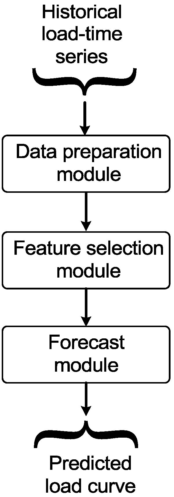
3. Our Proposed Work

Subject to the complex day-ahead load forecast of SGs, any proposed prediction strategy should be capable enough to mitigate the non-linear input/output relationship as efficiently as possible. We choose an ANN-based forecaster for two reasons; (i) these can capture non-linearity in historical load data; and (ii) the flexibility and ease in implementation with acceptable accuracy (note: both of these reasons are justified via simulations). However, prior to ANN-based forecasting, input load time series must be made compatible. Therefore, our proposed day-ahead load forecasting model (for SGs) consists of three modules: the data preparation module, the feature selection module and the forecast module (refer to Figure 2). The first module performs pre-processing to make the input data compatible with the feature selection module and the forecast module. The second module removes irrelevant and redundant features from the input data. The third module consists of an ANN to forecast the day-ahead load of the SG. The details are as follows.
Figure 2. Block diagram of the proposed methodology.
Applsci 05 01756 g002

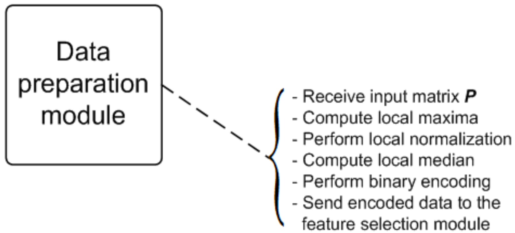
3.1. Pre-Processing Module

Suppose that the input load time series is shown by the following matrix:
P = p h 1 d 1 p h 2 d 1 p h 3 d 1 p h m d 1 p h 1 d 2 p h 2 d 2 p h 3 d 2 p h m d 2 p h 1 d 3 p h 2 d 3 p h 3 d 3 p h m d 3 p h 1 d n p h 2 d n p h 3 d n p h m d n
where h m is the m-th hour, d n is the n-th day and p h m d n is the historical power consumption value at the m-th hour of the n-th day. As there are 24 h in a day, m = 24 . The value of n depends on the designer’s choice, i.e., a greater value of n leads to fine tuning during the training process of the forecast module, because more lagged samples of input data are available. However, this would lead to greater execution time.
Prior to feeding the feature selection module with input matrix P, the following step-wise operations are performed by the data preparation module (refer to Figure 3):
  • Local maximum: Initially, a local maximum value is calculated for each column of the P matrix; p m a x c i = m a x { p h i d 1 , p h i d 2 , p h i d 3 , , p h i d n } , i { 1 , 2 , 3 , , n } .
  • Local normalization: In this step, each column of the matrix P is normalized by its respective local maxima, such that the resultant matrix is represented by P n r m . Now, each entry of P n r m ranges between zero and one.
  • Local median: For each column of the P n r m matrix, a local median value M e d i is calculated ( i { 1 , 2 , 3 , , n } ).
  • Binary encoding: Each entry of the P n r m matrix is compared to its respective M e d i value. If the entry is less than its respective local median value, then it is encoded with a binary zero; else, it is encoded with a binary one. In this way, a resultant matrix containing only binary values (zeroes and ones), P b , is obtained.
Figure 3. Data preparation module.
Applsci 05 01756 g003
Note: the load/consumption pattern is different for different days, i.e., the load pattern on holidays is different from that on working days. In order to enhance the accuracy of prediction strategy, the training samples must be relevant. Similarly, a lesser number of training samples will decrease the execution time of the prediction strategy. The above two reasons lead us to prefer local normalization over global normalization.
At this stage, the P b matrix is compatible with the feature selection module and is thus fed into it.

3.2. Feature Selection Module

Once the data are binary encoded, not only redundant, but also irrelevant samples need to be removed from the lagged input data samples. In removing redundant features, the execution time during the training process is minimized. On the other hand, removal of irrelevant features leads to improvement in forecast accuracy, because the outliers are removed.
In order to remove the irrelevant and redundant features from the binary encoded input data matrix P b , an entropy-based mutual information technique is used in [9,12], which defines the mutual information between input Q and target T by the following formula,
M I ( Q , T ) = i j p ( Q i , T j ) l o g 2 p ( Q i , T j ) p ( Q i ) p ( T i ) i , j { 0 , 1 }
In Equation (2), M I ( Q , T ) = 0 means that Q and T are independent; a high value of M I ( Q , T ) means that Q and T are strongly related, and a low value of M I ( Q , T ) means that Q and T are loosely related.
Thus, the candidate inputs are ranked with respect to the mutual information value between input and target values. In [9,12], the target values are chosen as the last samples for every hour of the day among all of the training samples (for every hour, only one target value is chosen that is the value of the previous day). The choice of the last sample seems logical, as it is the closest value to the upcoming day with respect to time; however, it may lead to serious forecast errors due to the lack of consideration of the average behaviour. However, consideration of only the average behaviour is also insufficient, because the last sample has its own importance. To sum up, we come up with a solution that not only considers the last sample, but also the average behaviour. Thus, we modify Equation (2) for three discrete random variables as,
M I ( Q , T , M ) = i j k p ( Q i , T j , M k ) l o g 2 p ( Q i , T j , M k ) p ( Q i ) p ( T i ) p ( M k ) i , j { 0 , 1 }
In expanded form, Equation (3) is written as follows,
M I ( Q , T , M ) = p ( Q = 0 , T = 0 , M = 0 ) × l o g 2 p ( Q = 0 , T = 0 , M = 0 p ( Q = 0 ) p ( T = 0 ) p ( M = 0 ) + p ( Q = 0 , T = 0 , M = 1 ) × l o g 2 p ( Q = 0 , T = 0 , M = 1 p ( Q = 0 ) p ( T = 0 ) p ( M = 1 ) + p ( Q = 0 , T = 1 , M = 0 ) × l o g 2 p ( Q = 0 , T = 1 , M = 0 p ( Q = 0 ) p ( T = 1 ) p ( M = 0 ) + p ( Q = 0 , T = 1 , M = 1 ) × l o g 2 p ( Q = 0 , T = 1 , M = 1 p ( Q = 0 ) p ( T = 1 ) p ( M = 1 ) + p ( Q = 1 , T = 0 , M = 0 ) × l o g 2 p ( Q = 1 , T = 0 , M = 0 ) p ( Q = 1 ) p ( T = 0 ) p ( M = 0 ) + p ( Q = 1 , T = 0 , M = 1 ) × l o g 2 p ( Q = 1 , T = 0 , M = 1 ) p ( Q = 1 ) p ( T = 0 ) p ( M = 1 ) + p ( Q = 1 , T = 1 , M = 0 ) × l o g 2 p ( Q = 1 , T = 1 , M = 0 ) p ( Q = 1 ) p ( T = 1 ) p ( M = 0 ) + p ( Q = 1 , T = 1 , M = 1 ) × l o g 2 p ( Q = 1 , T = 1 , M = 1 ) p ( Q = 1 ) p ( T = 1 ) p ( M = 1 )
In order to determine the M I value between Q and T, the joint and independent probabilities need to be determined. For this purpose, an auxiliary variable A v is introduced.
A v = 4 T + 2 M + Q T , M , Q { 0 , 1 }
It is clear from Equation (5) that A v ranges between zero and seven. A 0 v , A 1 v , A 2 v , A 3 v , ..., A 7 v counts the number of sample data points (out of total l data points) for which A v = 0 , A v = 1 , A v = 2 , A v = 3 ,..., A v = 7 , respectively. In this way, we can now easily determine the joint and independent probabilities as follows.
p ( Q = 0 , T = 0 , M = 0 ) = A 0 v l p ( Q = 0 , T = 0 , M = 1 ) = A 2 v l p ( Q = 0 , T = 1 , M = 0 ) = A 4 v l p ( Q = 0 , T = 1 , M = 1 ) = A 6 v l p ( Q = 1 , T = 0 , M = 0 ) = A 1 v l p ( Q = 1 , T = 0 , M = 1 ) = A 3 v l p ( Q = 1 , T = 1 , M = 0 ) = A 5 v l p ( Q = 1 , T = 1 , M = 1 ) = A 7 v l
p ( Q = 0 ) = A 0 v + A 2 v + A 4 v + A 6 v l p ( Q = 1 ) = A 1 v + A 3 v + A 5 v + A 7 v l p ( T = 0 ) = A 0 v + A 1 v + A 2 v + A 3 v l p ( T = 1 ) = A 4 v + A 4 v + A 5 v + A 7 v l p ( M = 0 ) = A 0 v + A 1 v + A 4 v + A 5 v l p ( M = 1 ) = A 2 v + A 3 v + A 6 v + A 7 v l
Based on Equation (4), mutual information between Q and T is calculated, and thus, redundancy and irrelevancy are removed from the input samples. This mutual information-based technique is computed with a reasonable execution time and acceptable accuracy.

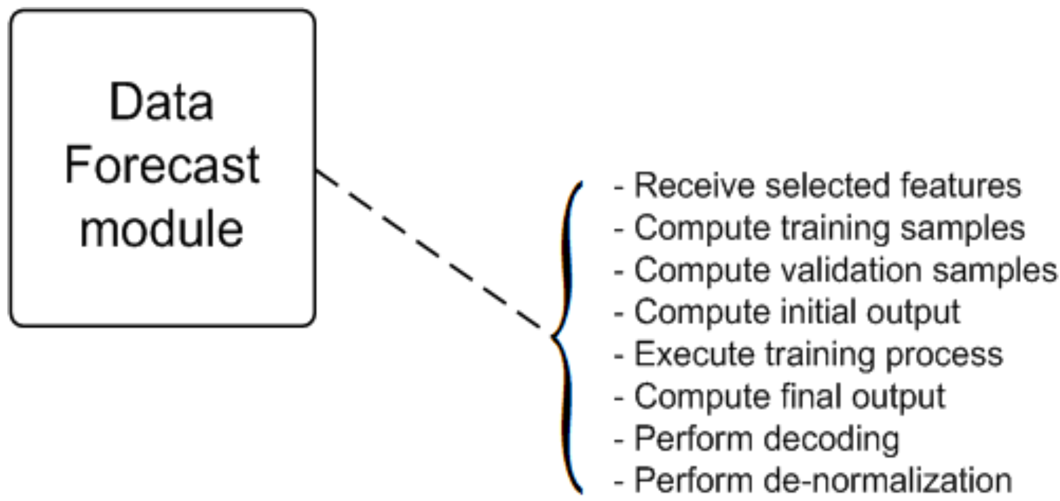
3.3. Forecast Module

By evaluating load variations over several months, or between two consecutive days, or between consecutive hours over a day, [16] concluded that SG’s load time series signal exhibits strong volatility and randomness. This result is obvious, because different users have different energy/power consumption patterns/habits. Thus, in terms of DLF, realization of an SG is more difficult as compared to its realization in terms of long-term load forecast. Therefore, the basic requirement of the forecast module is to forecast the load time series of an SG by taking into consideration its non-linear characteristics. In this regard, ANNs are widely used for two reasons; accurate forecast ability and the ability to capture the non-linear characteristics.
Due to the aforementioned reasons, we choose an ANN-based implementation in our forecast module. Initially, the forecast module receives selected features S F ( . ) and then constructs training “ T S ” and validation samples “ V S ” from it as follows:
T S = S F ( i , j ) , i { 2 , 3 , , m } a n d j { 1 , 2 , 3 , , n }
V S = S F ( 1 , j ) , j { 1 , 2 , 3 , , n }
From Equations (8) and (9), it is clear that the ANN is trained by all of the historical load time series candidates, except the last one, which is used for validation purpose. This discussion leads us towards the explanation of the training mechanism. However, prior to the explanation, it is essential to describe the ANN.
An ANN, inspired by the nervous system of humans, is a set of artificial neurons (ANs) to perform the tasks of interest (note: our task of interest is the DLF of SGs). Usually, an AN performs a non-linear mapping from R I to [ 0 , 1 ] that depends on the activation function used.
f a c t A N : R I [ 0 , 1 ]
where I is the vector of the input signal to the AN (here, inputs are the selected features only). Figure 4 illustrates the structure of an AN that receives I = ( I 1 , I 2 , , I n ) . In order to either deplete or strengthen the input signal, to each I i is associated a weight w i . The ANN computes I and uses f a c t A N to compute the output signal “y”. However, the strength of y is also influenced by a bias value (threshold) “b”. Therefore, we can compute I as follows:
I = i = 1 i m a x I i w i
The f a c t A N receives I and b to determine y. Generally, f a c t A N ’s are mappings that monotonically increase ( f a c t A N ( - = 0 ) and f a c t A N ( + = 1 ) ). Among the typically used f a c t A N ’s, we use sigmoid f a c t A N .
f a c t A N ( I , b ) = 1 1 + e - α ( I - b )
We choose sigmoid f a c t A N due for two reasons; f a c t A N ( 0 , 1 ) , and the parameter α has the ability to control the steepness of the f a c t A N . In other words, the sigmoid f a c t A N choice enables the AN to capture the non-linear characteristic of load time series. Since this work aims at the DLF for SGs, and one day consists of 24 h, the ANN consists of 24 forecasters (one AN for an hour), where each forecaster predicts the load of one hour of the next day. In other words, 24 hourly load time series are separately modelled instead of one complex forecaster. The whole process is repeated every day to forecast the load of the next day.
Figure 4. An artificial neuron.
Applsci 05 01756 g004
The question that now needs to be answered is how to determine w i and b? The answer is straight forward, i.e., via learning. In our case, prior knowledge of load-time series exists. Thereby, we use supervised learning; adjusting w i and b values until a certain termination criterion is satisfied. The basic objective of supervised training is to adjust w i and b such that the error signal “ e ( k ) ” between the target value “ y ^ ( k ) ” and real output of neuron “ y ( k ) ” is minimized.
M i n i m i z e e ( k ) = y ( k ) - y ^ ( k ) , k { 1 , 2 , 3 , , m }
We use the method of least squares to determine the parameter matrices, which is given as follows,
M i n i m i z e J = k = 1 m e T ( k ) e ( k ) , k { 1 , 2 , 3 , , m }
Subject to the most feasible solution of Equation (14), we use the multi-variate auto-regressive model presented in [17], because it solves the objective function in relatively less time with reasonable accuracy, as compared to the typically used learning rules, like gradient descent, Widrow–Hoff and delta [18]. According to [17], the parameter matrices are given as follows,
i = 1 n W ( i ) R ( j - i ) = 0 , j = { 2 , 3 , , n }
i = 1 n W ¯ ( i ) R ( i - j ) = 0 , j = { 2 , 3 , , n }
where W ( 1 ) = I D ( I D is the identity matrix), W ¯ ( 1 ) = I D and R is the cross co-relation given as:
R ( i ) = 1 n k = i n - 1 - i [ x ( k ) - m ] [ x ( k - i ) - m ] T
In Equation (11), m is the mean vector of the observed data,
m = 1 n k = i n x ( k )
Based on these equations, [17] defines the following prediction error co-variance matrices.
V t = k = 1 n W t ( k ) R ( k ) V ¯ t = k = 1 n W ¯ t ( k ) R ( k ) Δ t = k = 1 n W t ( k ) R ( t k + 1 ) Δ ¯ t = k = 1 n W ¯ t ( k ) R ( t + k 1 ) }
The recursive equations are as follows:
W t + 1 ( k ) = W t ( k ) W t + 1 ( t + 1 ) W t ¯ ( t k + 1 ) W ¯ t + 1 ( k ) = W ¯ t ( k ) W ¯ t + 1 ( t + 1 ) W t ¯ ( t k + 1 )   }
W t + 1 ( t + 1 ) = Δ t V ¯ t 1 W ¯ t + 1 ( t + 1 ) = Δ ¯ t V t 1   }
In order to find the weights, Equations (20) and (21) are solved recursively. For further details about the weight update mechanism, Equations (15)–(21), readers are suggested to read [17]. Figure 5 is a pictorial representation of the steps involved in the data forecast module.
Figure 5. Data forecast module.
Applsci 05 01756 g005
Once the weights in Equations (20) and (21) are recursively adjusted as per the objective function in Equation (13), the output matrix is then binary decoded and de-normalized to get the desired load time series. The stepwise algorithm of the proposed methodology is shown in Algorithm 1.
Algorithm 1 Day-ahead load forecast.
1:
Pre-conditions: i = number of days, and j = number of hours per day
2:
P historical load data
3:
Compute P m a x c i i { 1 , 2 , 3 , , n }
4:
Compute P n r m
5:
Compute M e d i i { 1 , 2 , 3 , , n }
6:
for all ( i { 1 , 2 , 3 , , n } ) do
7:
  for all ( j { 1 , 2 , 3 , , m } ) do
8:
      if ( P n r m ( i , j ) M e d i ) then
9:
             P b i , j 0
10:
      else if then
11:
             P b i , j 1
12:
      end if
13:
  end for
14:
end for
15:
Remove redundant and irrelevant features using Equation (4)
16:
Compute T S and V S using Equations (8) and (9), respectively
17:
Compute y ( 1 ) by letting W ( 1 ) = I and W ¯ ( 1 ) = I
18:
while Maximum number of iterations not reached do
19:
  if J ( k + 1 ) J ( k ) then
20:
       y ( k ) y ( k + 1 )
21:
  else if then
22:
      Train ANN as per Equations (20) and (21)
23:
      Compute y ( k + 1 ) and go back to Step (18)
24:
  end if
25:
end while
26:
Perform decoding
27:
Perform de-normalization
Note: our proposed prediction model predicts tomorrow’s load on the basis of historical load till today. Thus, the prediction model never fails, i.e., for every next day, the model needs information till the current day. However, the proposed model is unable to predict the load for more than tomorrow provided the historical load information till today.

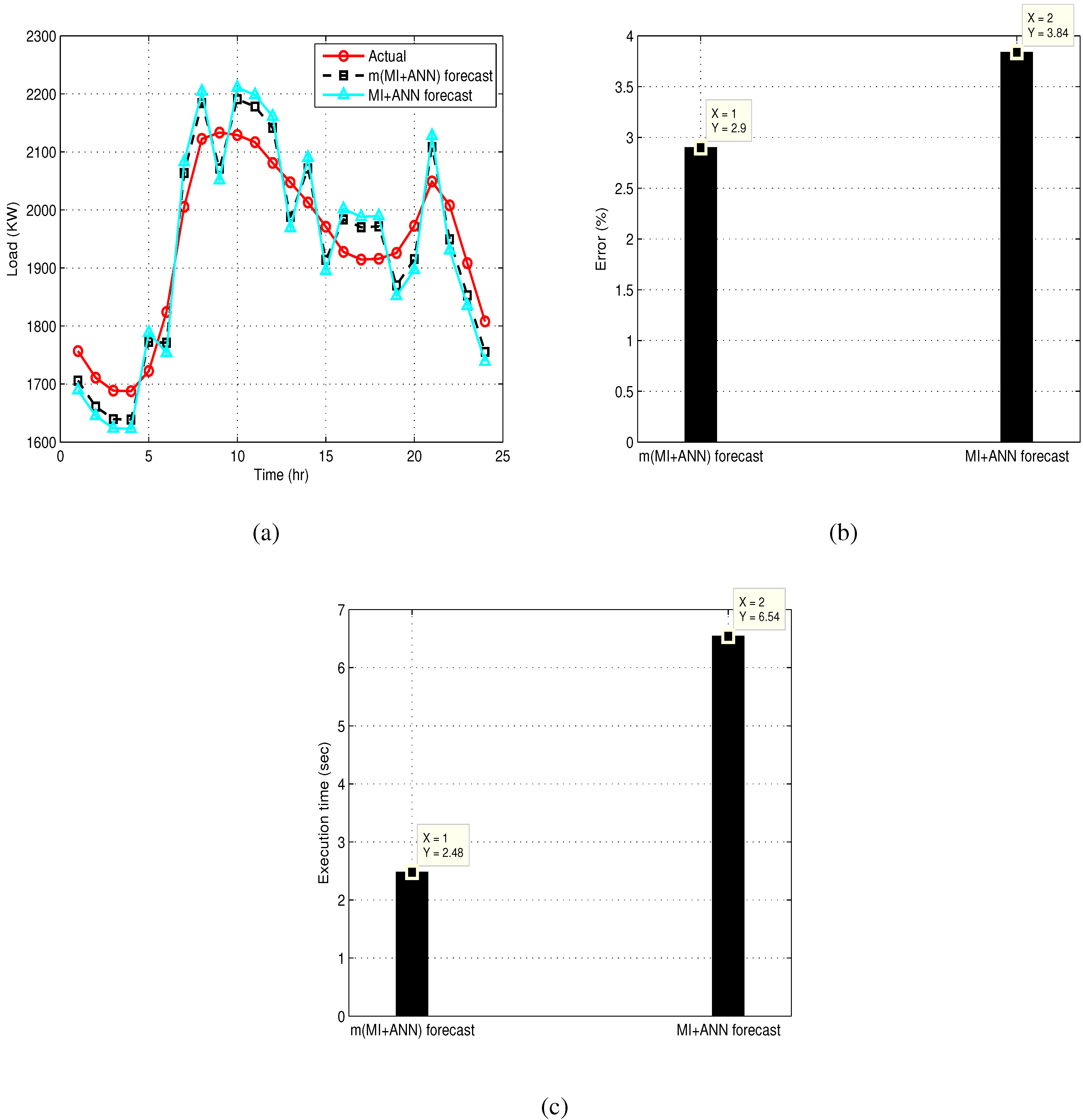
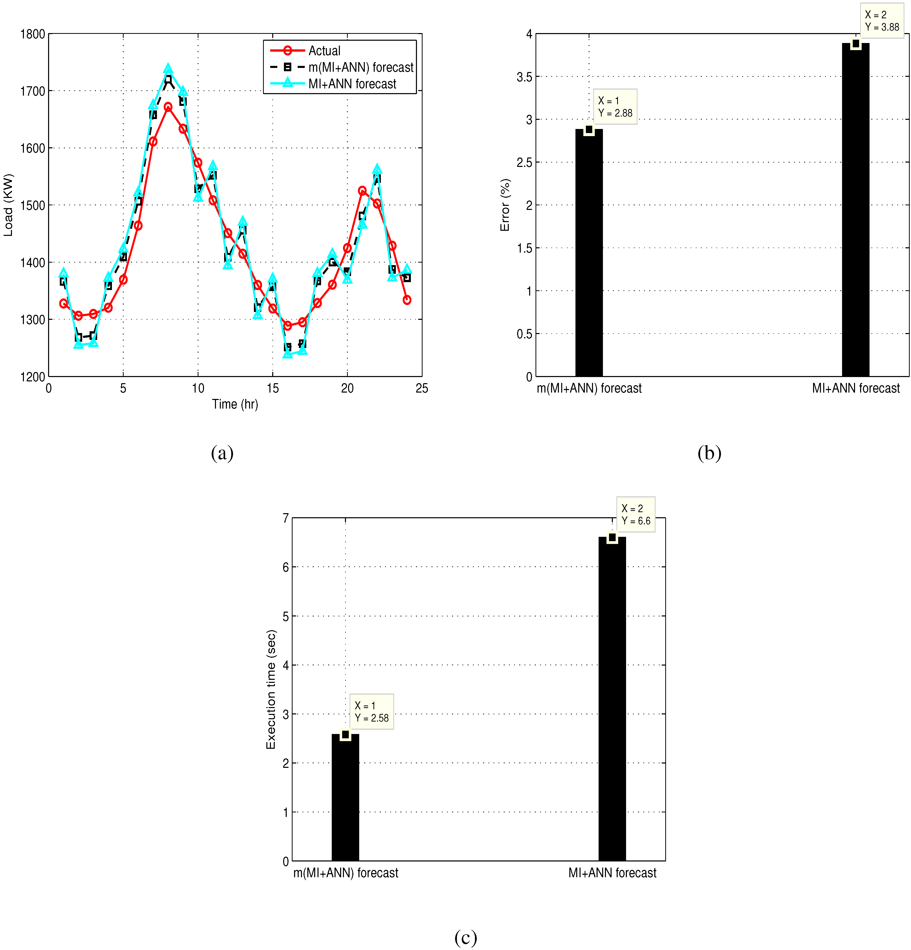
4. Simulation Results

We evaluate our proposed DLF model (m(MI + ANN)) by comparing it with an existing MI + ANN model in [12]. We choose the existing MI + ANN model in [12] for comparison, because its architecture has a close resemblance to our proposed model. In our simulations, historical load time series data from November (2014) to January (2015) are taken from the publicly-available PJM electricity market for two SGs in the United States of America; DAYTOWN and EKPC [19]. November to December (2014) data are used for training and validation purposes, and January (2015) data are used for testing purposes. Simulation parameters are shown in Table 1, and their justification can be found in [9,12,17,18]. In this paper, we have considered two performance metrics; % error and execution time (convergence rate).
  • Error performance: This is the difference between the actual and the forecast signal/curve and is measured in %.
  • Convergence rate or execution time: This is the simulation time taken by the system to execute a specific forecast model. Forecast models for which the execution time is small are said to converge quickly as compared to the opposite case. In this paper, execution time is measured in seconds.
Table 1. Simulation parameters.
ParameterValue
Number of forecasters24
Number of hidden layers1
Number of neurons in the hidden unit5
Number of iterations100
Momentum0
Initial weights 0 . 1
Historical load data26 days
Bias value0
Figure 6a and Figure 7a are the graphical illustrations of how well our proposed ANN-based DALF model predicts the target values of an SG. In these figures, the proposed m(MI + ANN)-based forecast curve more tightly follows the target curve as compared to the existing MI + ANN-based forecast curve, which is justification of the theoretical discussion of our proposed methodology in terms of non-linear forecast ability. Not only the sigmoid f a c t A N (refer to equation), but also the multivariate auto-regressive training algorithm enable the day-ahead ANN-based forecast methodology to capture non-linearity(ies) in historical load data.
Figure 6b shows the % forecast error when tests are conducted on the DAYTOWN grid; our m(MI + ANN) forecasts with 2 . 9 % and the existing MI + ANN forecasts with 3 . 84 % relative errors, respectively. Similarly, Figure 7b shows the % forecast error when tests are conducted on the EKPC grid; our m(MI + ANN) forecasts with 2 . 88 % and the existing MI + ANN forecasts with 3 . 88 % relative errors, respectively. This improvement in terms of relative % error performance by our proposed DALF model is due to the following two reasons: (i) the modified feature selection technique in our proposed DALF model; and (ii) multi-variate auto-regressive training algorithm. The first reason accounts for the removal of redundant, as well as irrelevant features from the input data in a more efficient way as compared to the existing DALF model. By a more efficient way, we mean that as our proposal considers the average sample in the feature selection process, as well in addition to the last sample and the target sample. Thus, the margin of outliers that cause significant relative % error is down-sized. The second reason deals with the selection of an efficient training algorithm, as our proposition trains the ANN via the multi-variate auto-regressive algorithm and the existing DALF model trains the ANN via Levenberg–Marquardt algorithm.
Figure 6. DAYTOWN (27 January 2015): m(MI + ANN) forecast vs. MI + ANN forecast. (a) Actual vs. forecast; (b) error performance; (c) convergence rate analysis.
Applsci 05 01756 g006
As discussed in Section 1, Section 2 and Section 3 that there exist a trade-off between forecast accuracy and execution time. However, Figure 6b,c and Figure 7b,c show that our proposed DALF model not only results in relatively less % error but also less execution time. As mentioned earlier, our devised modifications in the feature selection process and selection of the multi variate training algorithm cause relative improvement in terms of % error. On the other hand, m(MI + ANN) model converges with a faster rate (less execution time) as compared to the existing MI + AN model due to three reasons; (i) exclusion of the local optimization algorithm subject to error minimization; (ii) modified feature selection process; and (iii) selection of multi variate auto regressive training algorithm. Quantitatively (Figure 6c and Figure 7c), the execution time of existing model is 6 . 54 s for DAYTOWN grid and 6 . 60 s for EKPC grid, and that of our proposed model is 2 . 48 s for DAYTOWN and 2 . 58 s for EKPC, respectively. In these figures, the relative improvement in execution time is 37 . 92 % for DAYTOWN, 39 . 09 % for EKPC. Our proposition selects features from the input data while considering average sample, last sample and the target sample. This means that the chances of outliers in selected features have been significantly decreased, and the local optimization algorithm used by the existing MI + ANN forecast model is not further needed. Our proposed m(MI + ANN) forecast model does not account for the execution time taken by the iterative optimization algorithm. As a result, our proposed DALF model converges with a faster rate as compared to the existing DALF model.
Figure 7. EKPC (27 January 2015): m(MI + ANN) forecast vs. MI + ANN forecast. (a) Actual vs. forecast; (b) Error performance; (c) Convergence rate analysis.
Applsci 05 01756 g007

5. Conclusion and Future Work

In SGs, current research work primarily focuses on optimization techniques of power scheduling. However, prior to scheduling, an accurate load forecasting model is needed, because accurate load forecasting leads to enhanced management of resources, which in turn directly affects the economies of the energy trade. Furthermore, lower similarities (high randomness) and non-linearity in history load curves make the SG’s DLF more challenging as compared to long-term load forecasting. Thus, the aforementioned reasons lead us to investigate the SG’s DLF models. From a literature review, we found that many DLF models are proposed for SGs; however, these models trade off between accuracy and execution time. Thus, we focus on the development of an accurate DLF model with reduced execution time. In this regard, this paper has presented an ANN-based DLF model for SGs. Simulation results show that the newly-proposed DLF model is able to capture the non-linearity(ies) in the history load curve, such that its accuracy is approximately 97 . 11 % , such that the average execution time is improved by 38 . 50 % .
As the multi-variate auto-regressive training model minimizes the forecast error to some extent, so our future directions are focused on either the improvement of this model or its replacement with a better model.

Acknowledgments

The authors would like to extend their sincere appreciation to the Visiting Professor Program at King Saud University for funding this research.

Author Contributions

All authors discussed and agreed on the idea and scientific contribution. Ashfaq Ahmad and Nadeem Javaid performed simulations and wrote simulation sections. Ashfaq Ahmad, Nadeem Javaid and Nabil Alrajeh did mathematical modeling in the manuscript. Ashfaq Ahmad, Zahoor Ali Khan, Umar Qasim and Abid Khan contributed in manuscript writing and revisions.

Conflicts of Interest

The authors declare no conflict of interest.

References

  1. Unveiling the Hidden Connections between E-mobility and Smart Microgrid. Available online: http://www.zeitgeistlab.ca/doc/Unveiling_the_Hidden_Connections_between_E-mobility_and_Smart_Microgrid.html (accessed on 20 February 2015).
  2. Yan, Y.; Qian, Y.; Sharif, H.; Tipper, D. A Survey on Smart Grid Communication Infrastructures: Motivations, Requirements and Challenges. IEEE Commun. Surv. Tutor. 2013, 15, 5–20. [Google Scholar] [CrossRef] [Green Version]
  3. Siano, P. Demand response and smart grids: A survey. Renew. Sustain. Energy Rev. 2014, 30, 461–478. [Google Scholar] [CrossRef]
  4. Mohassel, R.R.; Fung, A.; Mohammadi, F.; Raahemifar, K. A survey on advanced metering infrastructure. Int. J. Electr. Power Energy Syst. 2014, 63, 473–484. [Google Scholar] [CrossRef]
  5. Atzeni, I.; Ordonez, L.G.; Scutari, G.; Palomar, D.P.; Fonollosa, J.R. Demand-Side Management via Distributed Energy Generation and Storage Optimization. IEEE Trans. Smart Grid 2013, 4, 866–876. [Google Scholar] [CrossRef]
  6. Adika, C.O.; Wang, L. Autonomous Appliance Scheduling for Household Energy Management. IEEE Trans. Smart Grid 2014, 5, 673–682. [Google Scholar] [CrossRef]
  7. Koutsopoulos, I.; Tassiulas, L. Optimal Control Policies for Power Demand Scheduling in the Smart Grid. IEEE J. Sel. Areas Commun. 2012, 30, 1049–1060. [Google Scholar] [CrossRef]
  8. Hermanns, H.; Wiechmann, H. Demand-Response Management for Dependable Power Grids. Embed. Syst. Smart Appl. Energy Manag. 2013, 3, 1–22. [Google Scholar]
  9. Amjady, N.; Keynia, F.; Zareipour, H. Short-Term Load Forecast of Microgrids by a New Bilevel Prediction Strategy. IEEE Trans. Smart Grid 2010, 1, 286–294. [Google Scholar] [CrossRef]
  10. Gruber, J.K.; Prodanovic, M. Residential energy load profile generation using a probabilistic approach. In Proceedings of the 2012 UKSim-AMSS 6th European Modelling Symposium, Valetta, Malta, 14–16 November 2012; pp. 317–322.
  11. Kou, P.; Gao, F. A sparse heteroscedastic model for the probabilistic load forecasting in energy-intensive enterprises. Electr. Power Energy Syst. 2014, 55, 144–154. [Google Scholar] [CrossRef]
  12. Amjaday, N.; Keynia, F. Day-Ahead Price Forecasting of Electricity Markets by Mutual Information Technique and Cascaded Neuro-Evolutionary Algorithm. IEEE Trans. Power Syst. 2009, 24, 306–318. [Google Scholar] [CrossRef]
  13. Yang, H.T.; Liao, J.T.; Lin, C.I. A load forecasting method for HEMS applications. In Proceedings of 2013 IEEE Grenoble PowerTech (POWERTECH), Grenoble, France, 16–20 June 2013; pp. 1–6.
  14. Meidani, H.; Ghanem, R. Multiscale Markov models with random transitions for energy demand management. Energy Build. 2013, 61, 267–274. [Google Scholar] [CrossRef]
  15. Amjady, N.; Keynia, F. Electricity market price spike analysis by a hybrid data model and feature selection technique. Electr. Power Syst. Res. 2009, 80, 318–327. [Google Scholar] [CrossRef]
  16. Liu, N.; Tang, Q.; Zhang, J.; Fan, W.; Liu, J. A Hybrid Forecasting Model with Parameter Optimization for Short-term Load Forecasting of Micro-grids. Appl. Energy 2014, 129, 336–345. [Google Scholar] [CrossRef]
  17. Anderson, C.W.; Stolz, E.A.; Shamsunder, S. Multivariate autoregressive models for classification of spontaneous electroencephalographic signals during mental tasks. IEEE Trans. Biomed. Eng. 1998, 45, 277–286. [Google Scholar] [CrossRef] [PubMed]
  18. Engelbrecht, A.P. Computational Intelligence: An Introduction, 2nd ed.; John Wiley & Sons: Hoboken, NJ, USA, 2007. [Google Scholar]
  19. PJM Home Page. Available online: www.pjm.com (accessed on 8 December 2015).

