
Reflective Inverse Diffusion

1
Department of Engineering Physics, Air Force Institute of Technology, Wright-Patterson AFB, OH 45433, USA
2
Department of Physics, U.S. Air Force Academy, CO 80840, USA
3
Department of Mathematics & Statistics, Air Force Institute of Technology, Wright-Patterson AFB, OH 45433, USA
*
Author to whom correspondence should be addressed.
Appl. Sci. 2016, 6(12), 370; https://doi.org/10.3390/app6120370
Submission received: 8 September 2016
/
Revised: 12 November 2016
/
Accepted: 14 November 2016
/
Published: 24 November 2016
(This article belongs to the Section Optics and Lasers)
Abstract
:Phase front modulation was previously used to refocus light after transmission through scattering media. This process has been adapted here to work in reflection. A liquid crystal spatial light modulator is used to conjugate the phase scattering properties of diffuse reflectors to produce a converging phase front just after reflection. The resultant focused spot had intensity enhancement values between 13 and 122 depending on the type of reflector. The intensity enhancement of more specular materials was greater in the specular region, while diffuse reflector materials achieved a greater enhancement in non-specular regions, facilitating non-mechanical steering of the focused spot. Scalar wave optics modeling corroborates the experimental results.
1. Introduction
All materials scatter light, either in a transmissive manner or reflectively, to some degree. The ground work for imaging with scattered light was put forth by Freund in which the random scatter was treated as a complex field that interfered with incident light to produce speckle patterns. It was theorized that with properly-modified incident light, the scattering object could be used to simulate different optical devices, such as a lens or mirror [1]. There was no distinction between scattering by transmission or reflection.
Motivated by the biomedical community’s search for methods of imaging through biological tissues, phase modulation techniques have demonstrated the ability to shape a wavefront causing light to refocus to a single point after transmission through a scattering medium [2,3,4,5,6,7,8,9,10,11,12,13]. Just as Freund predicted a decade earlier, properly-modified incident light allowed the scattering medium to behave as a lens [1]. This process, called “inverse diffusion” by the authors, is also capable of simulating a phase grating that allows control of the focus spot location in the observation plane by adjusting the wavefront shape.
Reconstructing images from reflected light would provide the ability to see around corners and is a growing interest in the remote sensing and intelligence communities. Other methods for imaging with reflectively-scattered light require an illumination source in the occluded scene [14] or require an illumination source with a line of sight to the occluded scene [15]. This presents an application problem as access to the occluded scene may not be available. Reflective inverse diffusion provides a method for illuminating occluded scenes without direct access or line of sight. By refocusing light after reflection a simulated light source can be achieved from almost any scattering surface, satisfying the line of sight requirement of existing imaging techniques, such as dual photography [15].
We demonstrate reflective inverse diffusion using feedback-based wavefront shaping methods adapted from the original transmissive inverse diffusion research. Our method was successful at refocusing light after being scattered by diffusely-reflecting surfaces. It was tested on six different surface types and produced various levels of enhancement (as defined previously [9]). Phase modulation also provided a method of non-mechanical beam steering; the ability to control the location of the refocused spot in the observation plane using reflective inverse diffusion was also demonstrated.
2. Background
2.1. Reflective vs. Transmissive Inverse Diffusion
Light scattering, whether by transmission through or reflection from a medium, is a linear process. Despite the complexity and unknown material properties, it can be considered deterministic as long as the medium is static [13]. Therefore, the relationship developed for transmissive inverse diffusion for the observed total field in the target area is also valid for the reflective case. The field at the m-th observation plane segment is given by [8]:
where is the -th complex-valued element of the transmission/reflection matrix relating the light from the n-th spatial light modulator (SLM) segment to the m-th segment in the observation plane, and represents the amplitude and phase of the light from the n-th SLM segment. The source field is segmented by the SLM into segments and reflected off the scattering medium. The segments of the SLM are equally sized and arranged , thus . The field at each of the M segments in the observation plane consists of a linear combination of the fields from the segments of the SLM [8]. Normalizing Equation (1) to intensity, , and the observed intensity at the m-th observation plane segment is then:
Intensity enhancement was defined by Vellekoop for transmissive inverse diffusion as [10]:
which is a simple ratio of the average intensity of the optimized spot divided by the average intensity of the unoptimized random speckle [9]. For transmission through a random medium, the terms follow a statistically-independent complex circular Gaussian distribution [16] with properties that can be used to simplify Equation (3) and express the ideal intensity enhancement as a function of the total number of SLM segments [10],
The thin films of turbid media in transmissive experiments were modeled using a circular Gaussian distribution [8,9,10]. However, the multiple random paths light travels when transmitted through a scattering medium are not present in the reflection model. This lack of complex circular Gaussian statistics produces a different expression for ideal enhancement. Using a simplified geometric approximation, the surface properties are modeled as a constant average surface reflectivity and phase delay that is related to the reflector surface height fluctuations [17]. Using this model, Equation (2) is rewritten for the reflection case as:
where is the average surface reflectivity and is the phase delay caused by the surface height fluctuations of the material. All of the tested materials have surface height fluctuations spanning multiple wavelengths (see “Roughness”, Table 1); a Gaussian phase distribution with a standard deviation greater than a wavelength appears uniformly distributed when phase wrapped to the interval . Thus, the phase term of the reflector material, , is assumed to have a uniform distribution over . The intensity achieves a maximum value when the SLM phase delay is set to cancel the phase delay imposed by the surface height of the reflector, ,
where the angled brackets again denote the ensemble average.
The unoptimized random speckle background can be expressed as a fixed-length random phasor sum,
which can be written as a complex number with amplitude A and phase Θ,
where A and Θ are both random variables and is the second moment. The probability density function of A is given by [17],
where is the magnitude of the random phasor sum, from the two-dimensional joint characteristic function of the random phasor sum [17] and is the zero-order Bessel function of the first kind. As the number of SLM segments approaches infinity, (), the probably density function in Equation (9) becomes a Rayleigh distribution [17]. For , Mathematica® numerically approximated the second moment of Equation (9) as . Substituting the results from Equations (6) and (8) into Equation (3) shows that the ideal enhancement for reflective inverse diffusion is ,
2.2. Mathematical Model
Scalar diffraction theory was used to develop a mathematical description of reflective inverse diffusion. The propagation distances of the experiment are all inside the Fresnel zone; thus, the Rayleigh–Sommerfeld diffraction formula is used for propagation. The transfer function for Rayleigh–Sommerfeld diffraction is [18]:
where z is the propagation distance, λ is the optical wavelength, k is the wavenumber and and are the respective horizontal and vertical spatial frequencies of the source field. Using the transfer function to propagate the source field, , a distance z, the observed field is given by [19]:
where are the Cartesian coordinates orthogonal to z corresponding to the spatial frequencies .
The field at each pixel of the SLM when illuminated by a plane wave can be considered simply as the phase delay applied at that pixel. Using Equation (12), the field is propagated from the SLM to just prior to lens in Figure 1, normalized with constant phase terms removed,
where is the distance from the SLM to lens . The Fourier transform property of lens is then used to determine the field at the diffusely-reflecting sample located at the lens focus,
Lens L2causes a coordinate transformation to the plane, which is related to the spatial frequencies by and , where [18].
The field at the sample given by Equation (14) is multiplied by , which represents the phase scattering properties of the reflector. The result is then propagated to the charge-coupled device (CCD) in the observation plane using Equation (12):
where are the coordinate axes of the SLM and are the respective horizontal and vertical spatial frequencies of the field at the SLM. The coordinate axes of the reflective sample are , and are the respective horizontal and vertical spatial frequencies of the field at the reflector. The focal length of lens is f, and and are the distances from the SLM to the lens and the reflective sample to the CCD, respectively. This transform relationship is unique to the reflective inverse diffusion setup in Figure 1. Transmissive inverse diffusion uses microscope objectives on both sides of the scattering sample that re-image the light onto the CCD (see Figure 2 in [9]). The differences in the experimental setups create different transform relationships for reflective and transmissive inverse diffusion. However, since both processes are linear, Equation (1) is valid for both.
3. Materials and Methods
3.1. Laboratory Experiments
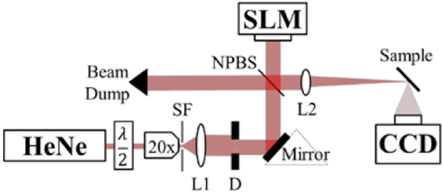
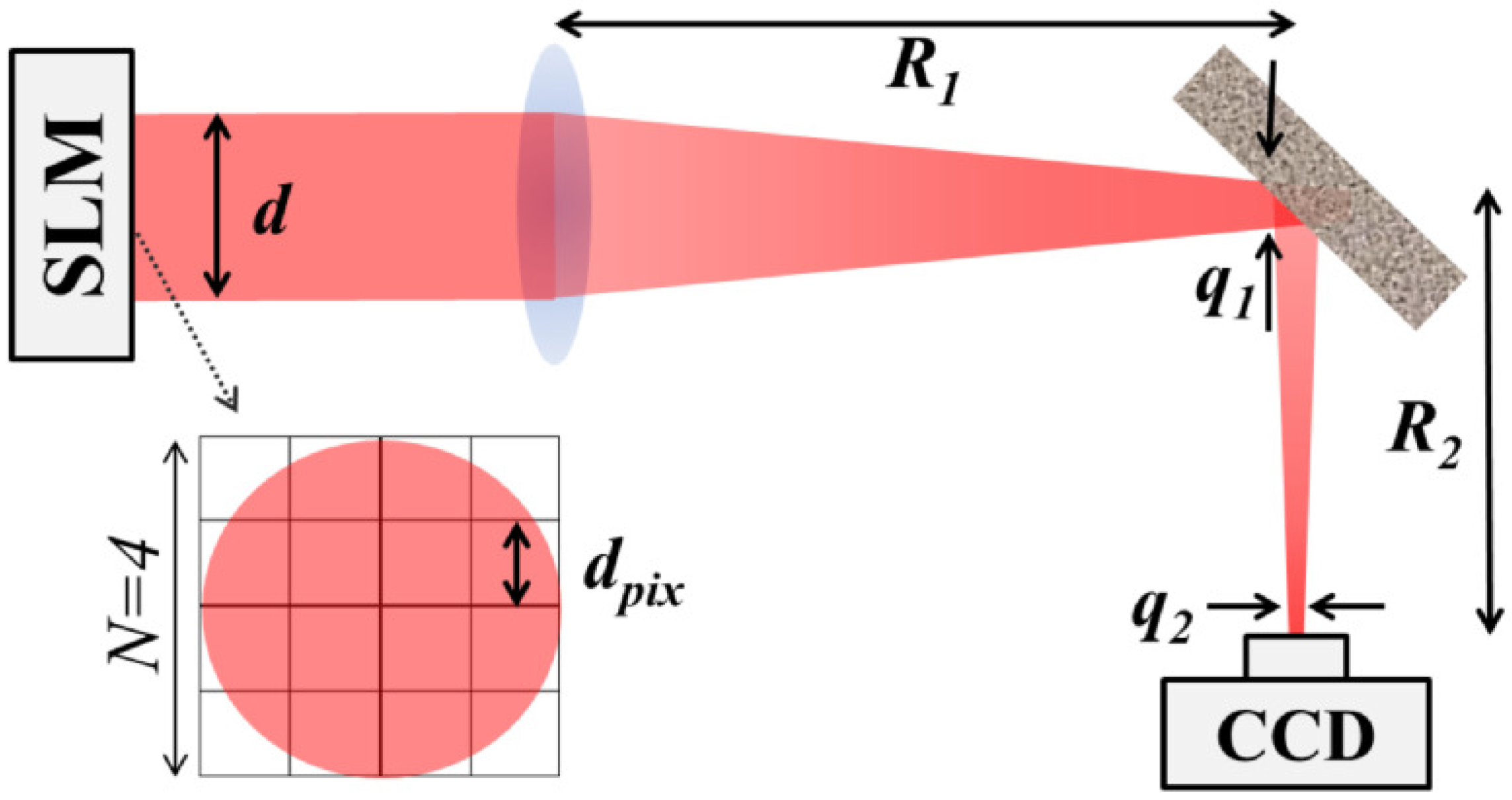
The experimental setup is shown in Figure 1. The primary components of the laboratory setup include a 30-mW HeNe laser (λ = 632.8 nm) with a semi-permanent neutral density filter attached. The filter had an optical density of 1.0 that reduced the effective power of the laser to approximately 3 mW, rendering it eye safe. Phase modulation is accomplished with a Boulder nonlinear systems (BNS) liquid crystal on silicon (LCoS) SLM. This reflective SLM is 7.68 mm by 7.68 mm, consisting of 512 by 512 pixels, each capable of 256 (8-bit) phase levels over a 2π phase stroke. Feedback is provided by a Santa Barbara Instruments Group (SBIG) ST-402ME CCD with 765 by 510 pixels and a pixel pitch of 9 m by 9 m.
The HeNe laser is first expanded and collimated to the width of the SLM using a microscope objective, spatial filter (SF) and lens . The non-polarizing beam splitter (NPBS) is used to allow for normal incidence on the SLM. After phase modulation, the beam is focused onto the reflective sample by lens with focal length, m. The phase-modulated beam is incident onto the diffusely-reflecting sample at 45. The reflector then scatters the incident beam onto the CCD placed 40 ± 0.5 cm from the reflector and at 45 from its surface normal.
The algorithm used to optimize the SLM is based on the continuous sequential algorithm developed for transmissive inverse diffusion [10]. The SLM is first segmented into segments of equal size. The phase of each segment is then cycled, and the target intensity is recorded by the CCD. The phase value of the segment is then set to produce the maximum target intensity at the desired location before moving on to the next SLM segment [10,11]. Pre-optimization with a smaller number of segments was performed before moving to sequentially, as it was shown to increase the signal-to-noise ratio in the transmissive experiments [9,11].
The reflective inverse diffusion algorithm was used for six different scattering materials: Spectralon®, brushed aluminum, sandblasted aluminum, Infragold®, white paint on glass and graphite. The reflector materials were selected based on the differences in the scattering properties. The surface roughness of the samples were measured and compared with the reflected spot enhancement produced by the algorithm. These measurements are shown in Table 1.
In addition to refocusing light after reflection, phase modulation demonstrated the ability to control the location of the focused spot in the observation plane. This non-mechanical beam steering technique required no initial changes to the experimental setup. The algorithm consecutively optimized and refocused light into each of the four corners of the CCD. The CCD was also translated in two dimensions while maintaining a fixed distance of 40 cm from the reflector to test the ability to refocus light over a larger target surface. For these experiments, the CCD was moved from the specular region of reflection into the diffuse region, defined as a horizontal shift of 66 mm and a vertical shift of 88 mm, or approximately and , respectively.
The most notable limitation of the test setup is the CCD. The maximum frame rate of the SBIG ST-402ME is approximately 1 frame per second. Adding the computational processing time, each intensity measurement takes approximately 1.5 s. A total of 21 phase values, equally spaced over the 0 to phase stroke of the SLM (), were tested, giving a total segment optimization time of approximately 32 s. Pre-optimization starting at N = 4 and progressing through N = 32 represents 1364 optimizations, with a total runtime of approximately 12 h. Since the SLM appeared to be slightly under-filled by the collimated laser beam, the number of optimizations was reduced by skipping segments in the far corners that are not expected to have an appreciable affect on the beam. This reduced a single experiment to 1160 optimizations with a total run time of approximately 10 h.
3.2. Simulations
A diffraction-based propagation model, discussed in Section 2.2, allowed for the examination of the field at any point in the simulation. Using MATLAB® to calculate the field at the CCD using Equation (15), an Intel Core i7® computer with 8 gigabytes of RAM could complete over 2 optimizations per second, which was more that 64-times faster than experimental methods with the available equipment. This model was validated using a mirror as a test case.
4. Results
4.1. Simulation Validation
The diffusely-reflecting sample was replaced by a mirror to validate the propagation-based simulation. In the simulation, the mirror is considered a perfect reflector, which eliminates the term from Equation (15). Qualitatively, with a mirror positioned at the focus of the positive lens, the creation of a focused spot on the CCD simply requires shifting the focus of the positive lens the distance from the mirror to the CCD. This is accomplished by applying a negative lens phase screen to the SLM. The phase screen for a lens is given by:
Using geometric optics, the focus of the negative lens is given by,
where is the distance from the SLM to the positive lens, is the distance from the lens to the mirror and also equal to the focal length of the positive lens and is the distance from the mirror to the CCD.
The spot produced by the mirror test case was captured by the CCD and compared with the spot simulated using Equation (15). Figure 2 shows both the measured and simulated spots and includes the center horizontal cross-sections of each. There was a 20-m difference between the FWHM diameter of the measured and simulated spots. The difference is attributed to uncertainties in the experimental distances between the SLM, lens, reflector and CCD that result in a small defocus error in the measured spot.
4.2. Speckle Size and Pre-Optimization
The SLM was segmented into segments, where , with random phase values applied to each segment and the speckle pattern recorded with the CCD. The speckle patterns in Figure 3 were produced by the sandblasted aluminum sample and show the variation of speckle pattern size as N is increased. All of the tested reflector materials showed a similar variation in speckle pattern size with respect to N. Simulated images are included in Figure 3 for comparison. They were generated using Equation (15) with the reflector term, , modeled as a uniform phase distribution with a magnitude of one. Histograms of the measured and simulated intensity speckle patterns fit a negative exponential probability density function, which is expected for fully-developed speckle [17]. A transmissive inverse diffusion experiment was conducted based on Vellekoop’s original research and used as a point of comparison. Using a white paint on glass sample as the scattering media, the size of the background speckle did not change with N. This was due to the imaging optics used and placed closely to the scattering sample.
The algorithm sequentially optimized the segments of the SLM to produce a focused spot on the CCD. For cases where , pre-optimization was accomplished, i.e., the SLM was optimized for each previous value of N. After each stage of optimizations, the algorithm proceeds to the next value of N by splitting each segment horizontally and vertically into four, equally-sized, smaller segments. These smaller segments are then individually re-optimized, and the process is repeated until the desired N is reached. The spot intensity produced by a pre-optimized SLM was compared to the spot produced by an SLM that was not pre-optimized. In addition, two different phase modulation step sizes, and , were used for the pre-optimization trials.
The results of pre-optimization for the graphite sample are shown in Figure 4. Pre-optimization did not appreciably affect the spot intensity for , but improved spot intensity for . An increase in peak intensity of approximately 40% is shown in the pre-optimized trial for . Computer simulations with a uniform phase reflector model showed a more modest effect with only a 5% increase in peak intensity in the pre-optimized trial for . A decrease in the phase modulation step size from to improved spot intensity by 20% for the graphite reflector and by 10% in simulation. Pre-optimization was shown to increase peak intensity for all of the reflector materials for . The amount of improvement was dependent on the individual material surface properties, such as roughness and correlation length. The exact relationship the material surface properties have on enhancement must be examined in future research.
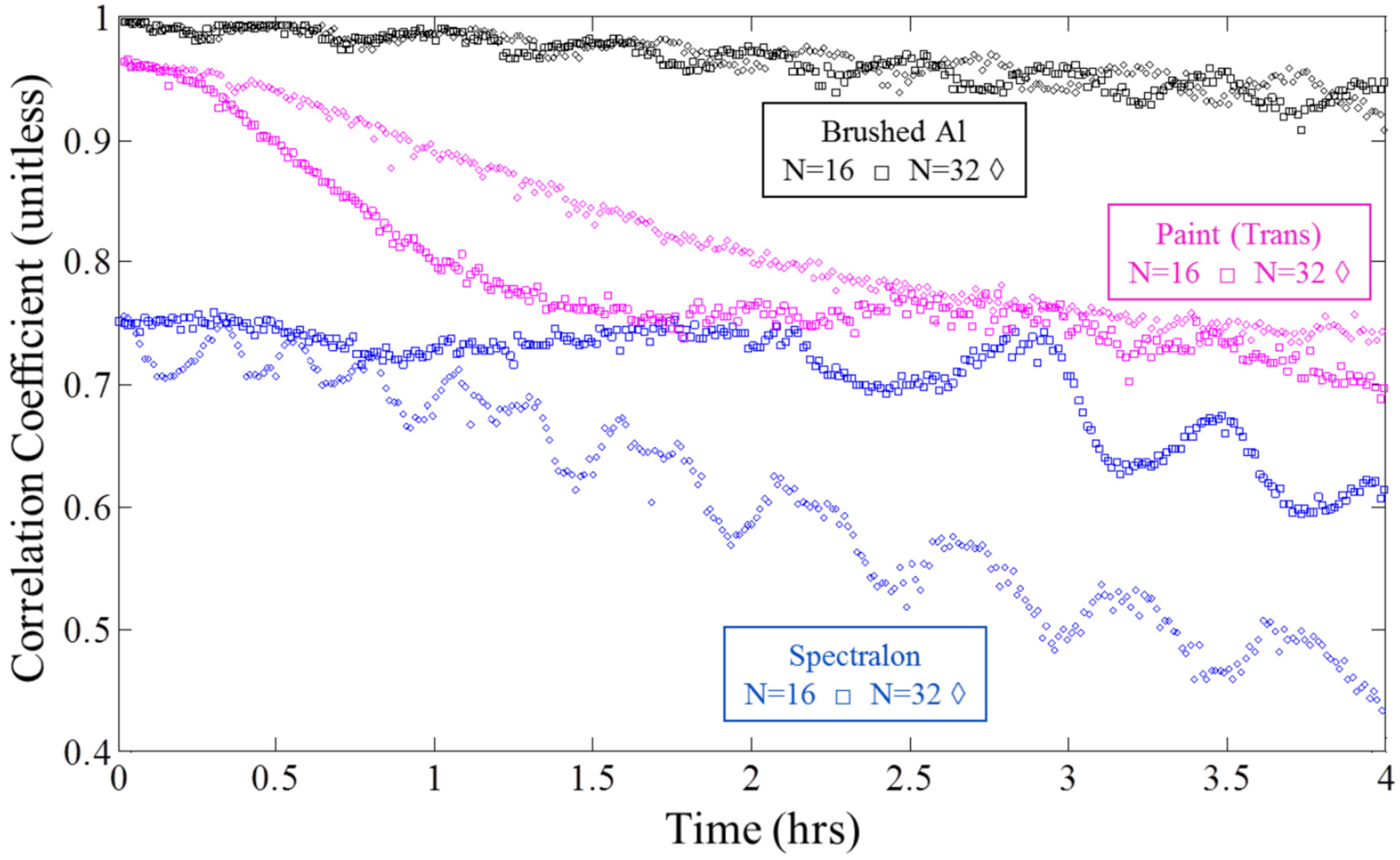
4.3. Speckle Pattern Decorrelation
The speckle pattern produced by a fixed SLM phase map and the diffusely-reflecting sample varied with time. The decorrelation of the speckle pattern is a function of both the material properties of the diffuse reflector and the laboratory test conditions. Figure 5 shows the correlation coefficient over time for the brushed aluminum, transmissive white paint and Spectralon® samples. As expected, the metal reflectors maintained a much higher correlation coefficient; thus, most of the decorrelation for the metal reflectors is attributed to the changing environmental conditions of the laboratory, such as temperature, air currents from the laboratory ventilation system, minute mechanical vibrations and device measurement error and noise. Previous work in the transmissive inverse diffusion shows enhancements () ranging from 50 to 1000 using both iterative and transmission matrix methods [3,4,6,9,20]. The cause of this wide range of enhancement values is still currently being investigated, with some of the disparity likely caused by noise [20].
The total noise in the system produced small, low frequency oscillations in the correlation coefficients plotted in Figure 5. The oscillation caused microscopic shifts in the reflector. This affected the correlation of the speckle produced by the volumetric scatterers, such as Spectralon® and the white paint samples, more than the metal reflectors due to the longer internal path length changes of the material. The depth of penetration of Spectralon® has been measured at 200 m for HeNe light [21], which is over 20-times the root mean square (RMS) roughness of any of the metal samples (see Table 1). The small shifts of the reflector in concert with the larger internal path length changes in the material caused Spectralon® to initially decorrelate much faster than the other samples. This decorrelation over time adds a degree of uncertainty to the process, where previously-optimized SLM segments are in fact suboptimal by the time the process is complete. These suboptimal segments cause a decrease in the overall spot enhancement. This decorrelation effect was simulated by adding a zero-mean Gaussian-distributed random phase, with a standard deviation between and , to the sample each time the intensity pattern was calculated. The standard deviation of the random phase was dependent on the severity of the decorrelation effect of the sample.
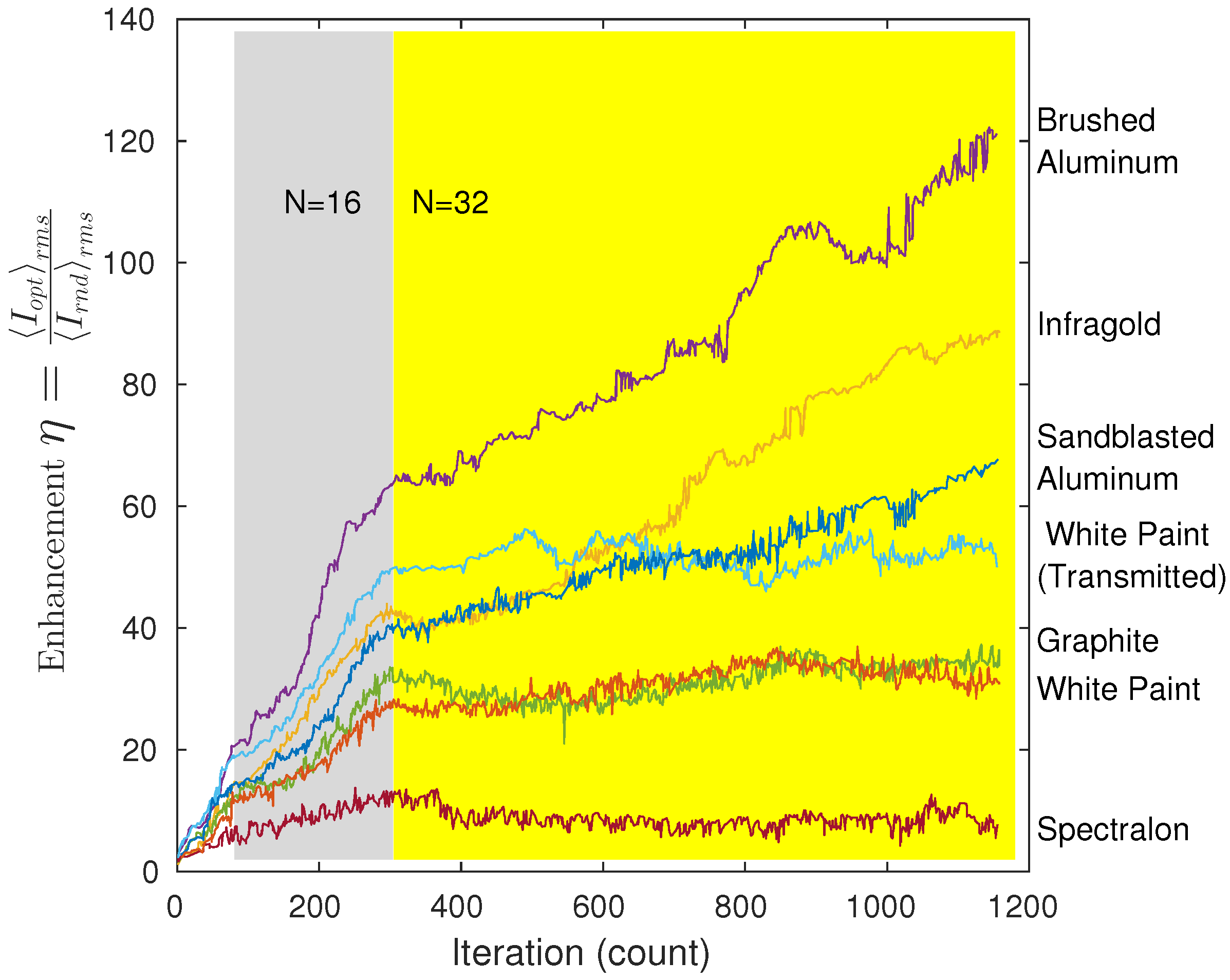
4.4. Reflector Materials
The spot intensity enhancement , measured surface roughness and final FWHM spot size are summarized in Table 1 for each of the reflector materials. The spot intensity is the RMS value of the CCD pixels inside the FWHM radius. The background intensity is the RMS value of the CCD pixels at a radius of three-times the FWHM and beyond.
The algorithm ran with pre-optimization starting with through for all six reflector materials. The spot enhancement was calculated after each segment was optimized and is shown in Figure 6. The smaller optimized segments in the case produced no improvement compared to the case for the graphite and Spectralon® reflectors. The enhancement for the white paint reflector continued to increase slowly during the initial segment optimization of the stage, but began to decrease midway through the optimization process. At the completion of the stage, the enhancement for the white paint reflector is only slightly higher than the enhancement.
Decorrelation is believed to be the cause for the lack of enhancement for the Spectralon® reflector. As a bulk scatterer rather than a surface reflector, Spectralon® causes light to undergo multiple scattering events before exiting. Studies have produced penetration depth estimates of 200 m for HeNe light in samples of Spectralon® [21]. This depth is approximately 20-times the thickness of the white paint sample used in transmissive inverse diffusion experiments, which indicates that larger internal path length changes occur in the Spectralon® sample.
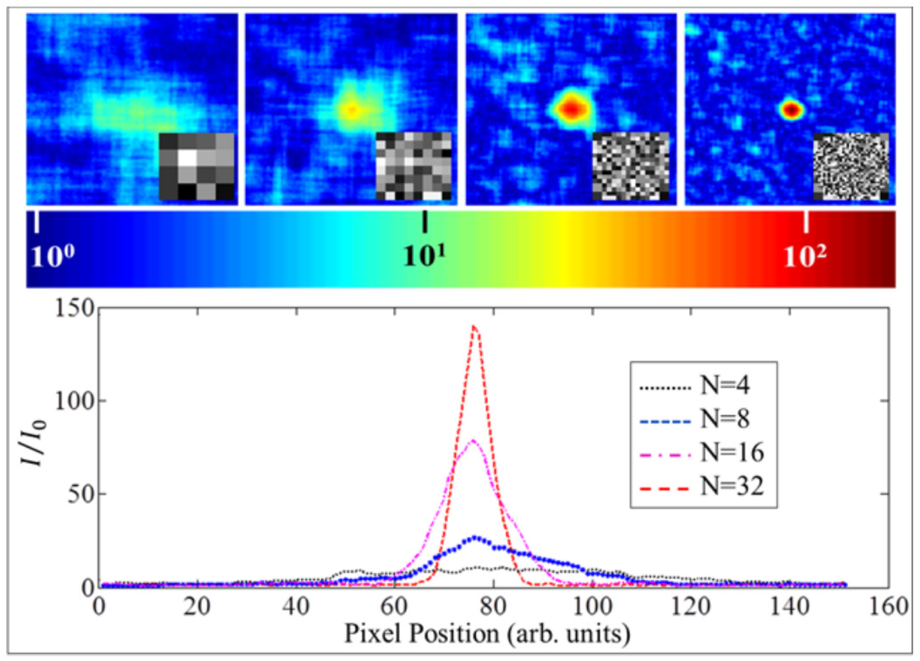
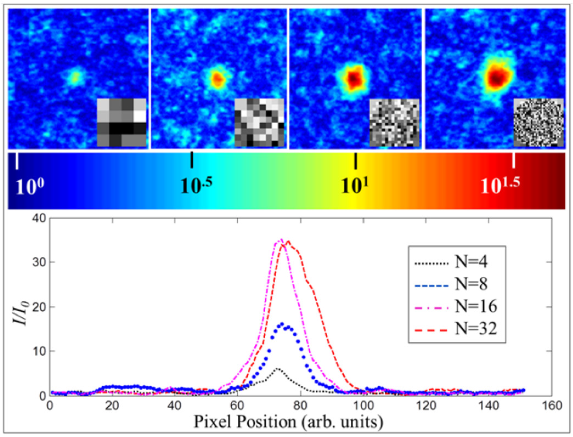
The greatest enhancement was achieved using the brushed aluminum reflector. The spot optimization for the brushed aluminum reflector is shown in Figure 7 along with the normalized intensity cross-section. The intensity cross-sections are shown as the algorithm completes each stage of optimizations. The cross-sections are normalized by the RMS intensity produced by a random phase map applied to the SLM.
A single transmissive inverse diffusion experiment was conducted based on Vellekoop’s experimental setup [9]. The white paint on glass sample was used for enhancement comparison between transmissive and reflective inverse diffusion. The results of the spot optimization and corresponding intensity cross-section are shown in Figure 8. In reflection, background speckle size decreased as N was increased; however, in the transmission trial, the background speckle was relatively constant for all N. The algorithm failed to produce additional enhancement during the stage for the baseline white paint transmission trial. Again, this is believed to be due to the decorrelation of the speckle pattern. The spot for the stage was larger than the previous spot. Decorrelation of the individual background speckles produced a smearing effect that produced an overall larger target spot.
As the algorithm completes each stage of optimizations, the enhancement is plotted as a function of total optimized SLM segments and compared with Equation (10). The results of a simulation using a uniformly-distributed random phase reflector model with reflectivity of one are show in Figure 9 without any added noise or decorrelations effects. The simulation and experimental data show similar trends, but less enhancement than predicted by Equation (10). This was expected and similar to transmission experiments [9], since the 21 phase values used for optimization represent an extremely small sample of the total phase space.
The enhancement predicted by the computer simulations corroborates the experimental data. The effects of speckle decorrelation were simulated by adding a zero-mean random Gaussian-distributed phase to the reflector model each time the intensity was calculated. The standard deviation () of the random phase fluctuation was dependent on the severity of decorrelation time of the material. Brushed aluminum maintained the highest correlation coefficient over time (see Figure 5), thus experiencing the lowest amount of enhancement loss attributed to speckle decorrelation. Simulations of the metal samples corresponded to a Gaussian phase fluctuation with standard deviation of to . The more diffuse samples, such as graphite and white paint, matched with a standard deviation of to . Figure 10 shows enhancement per iteration for a given standard deviation of the Gaussian phase fluctuation.
Spectralon®, with its high depth of light penetration and multiple reflections, was considered similar to the random paths experienced by light when transmitted through a scattering medium. Simulations of both the circular Gaussian model from transmissive inverse diffusion and uniform phase model produced similar enhancement with the same phase fluctuation standard deviation deviation of (see Figure 10). The enhancement for the uniform phase model does initially rise faster than the circular Gaussian model, which is expected based on the slopes of Equations (3) and (10). However, due to the decorrelation effects and limited number of phase values used in the optimization process, neither model was significantly better than the other at simulating the Spectralon® results.
4.5. Spot Size
The relationship between SLM dimension N and the background speckle size led to a corresponding relationship between N and the final focused spot size. The final spot size is approximated by applying diffraction theory to the light propagating from an individual SLM segment. The relevant dimensions are shown in Figure 11. Given that , the focal length of lens , the spot size at the reflector is approximated by,
where is the width of a single square SLM segment. The final spot dimension in the observation plane is approximated by,
where d is the width of the entire SLM.
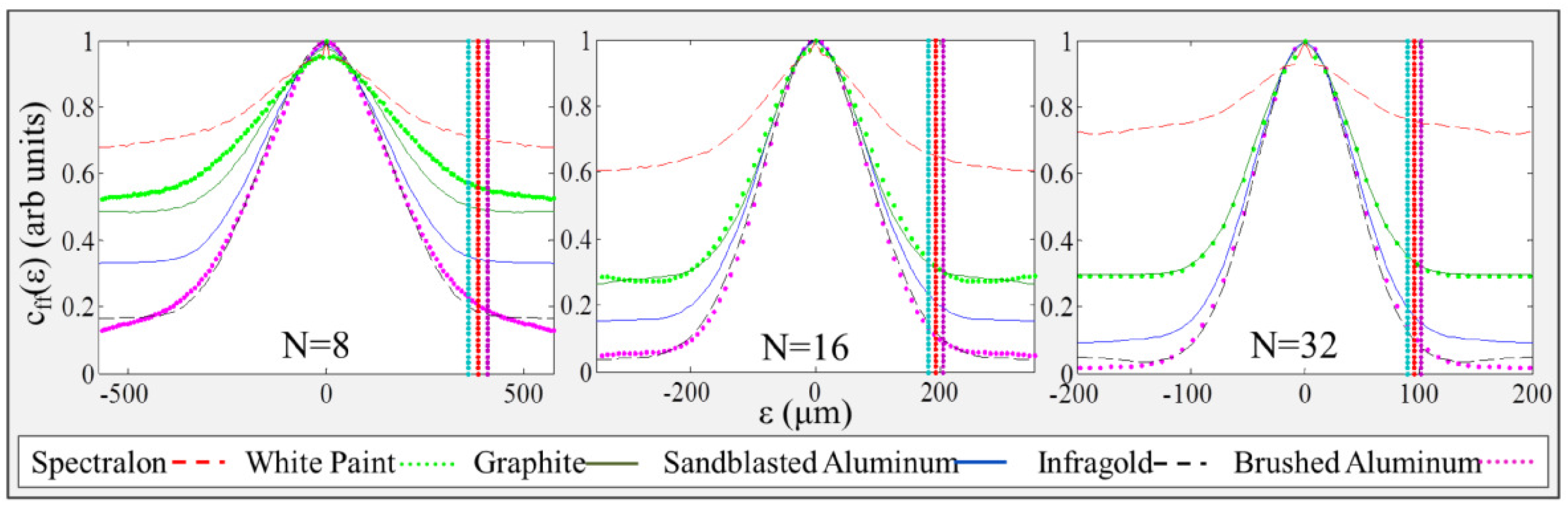
The spot size from the CCD was determined by a one-dimensional autocorrelation on the center row of pixels for the 8, 16 and 32 stages. The autocorrelation for each of the reflector materials is shown in Figure 12. The vertical lines in the figure mark the predicted size in red with upper and lower bounds of the measured spot in cyan and magenta, respectively. The measured full width from the CCD was consistent with the spot sizes predicted by Equation (19) of 384 m, 192 m and 96 m for 8, 16 and 32, respectively.
4.6. Non-Mechanical Beam Steering
Non-mechanical beam steering, in the context of reflective inverse diffusion, refers to the ability to change the location of the focus spot in the observation plane without any physical modification of the experiment setup; only phase modulation from the SLM was used. The algorithm, with pre-optimization for through 16, sequentially targeted the four corners of the CCD, which represents a deflection angle of . The enhancement of the four target corners was comparable with less than a 15% difference between maximum and minimum enhancement.
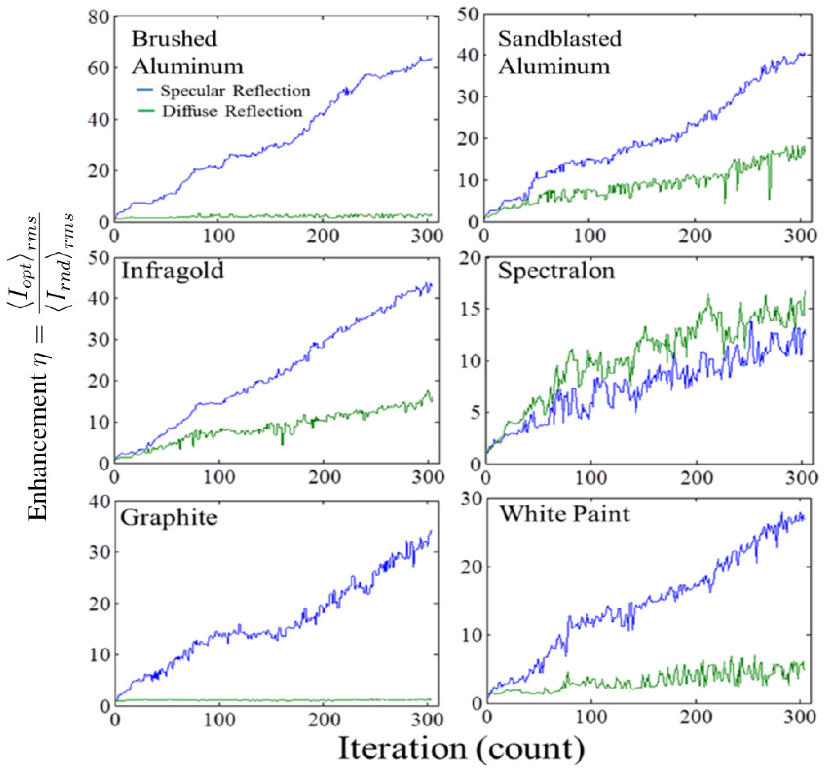
The size of a playing card with dimensions of 88 mm × 63 mm represents a maximum deflection angle of horizontally and vertically and was chosen to demonstrate beam steering over a larger angle. The brushed aluminum reflector lost almost 60% of peak spot enhancement when the target location moved the maximum diagonal dimension. The reduction in enhancement corresponds to the focus spot moving from the specular region of the bidirectional reflectance distribution function (BRDF) into the diffuse region.
The spot enhancement from the diffuse region of reflection was measured for each of the reflector materials and compared with its specular reflection results. The specular enhancement was measured using the same setup as described in Section 3.1, and the algorithm was allowed to run with pre-optimization from 2 through 16. The CCD was then moved to the diagonal displacement of 108.2 mm () to approximate the diffuse region of reflection while maintaining a distance of 40 ± 0.5 cm from the reflector. The algorithm was run with pre-optimization from 2 through 16. The results are plotted in Figure 13. Brushed aluminum achieved a specular enhancement of approximately 60, but only achieved an enhancement of approximately four in the diffuse region. The white paint and graphite reflectors both achieved a specular enhancement of approximately 30 and diffuse enhancements of approximately six and two, respectively. Sandblasted aluminum and Infragold® both achieved specular enhancements of approximately 40 and diffuse enhancements of 20. Spectralon® achieved a specular enhancement of 16 and a diffuse enhancement of 12, retaining 75% of its specular enhancement in the diffuse region due to its highly Lambertian reflective properties.
5. Conclusions
This research demonstrates reflective inverse diffusion. Just as transmissive inverse diffusion seeks to image through scattering media and biological tissues, the goal of reflective inverse diffusion is to investigate the possibility of imaging from reflective scattering media. Mathematical analysis based on diffraction theory was presented and provides propagation-based simulations that corroborate experimental results. In addition to proof-of-concept results, non-mechanical beam steering was demonstrated. Although it was shown that the reflective properties of the sample affect spot enhancement, the exact relationship that material properties, such as surface roughness and correlation length, have on enhancement is left for future work.
While our transmissive inverse diffusion experiment through white paint produced an enhancement of 56, reflective inverse diffusion using metallic reflectors produced enhancements between 67 and 122 in the specular region. The high specular reflectance and sample stability are factors that contributed to the larger enhancement levels. The more diffuse reflecting materials provided levels of enhancement lower than the transmission case, but produced enhancement over a wider scatter angle than the more specular samples.
Our continued research seeks to improve the experimental results with better equipment, namely the SLM and CCD, and better optimization algorithms, to expand simulation methods to better model noise and to further examine the relationship between specular and diffuse reflectance to provide a method for predicting enhancement. Better equipment and optimization algorithms are also expected to provide insight into the case of decorrelation observed in these samples. Just as matrix methods have been successfully implemented in transmission to allow near real-time control of the enhanced spot location [22], we are also investigating this for use in reflection. Future work will also include a polarization study. It is known that some reflectors depolarize light more than others, e.g., bulk versus surface scatterers. It is possible that polarization can be used to improve the reflective inverse diffusion results.
Acknowledgments
This work is supported by the Air Force Office of Scientific Research. The views expressed in this article are those of the authors and do not reflect the official policy or position of the United States Air Force, Department of Defense, or the United States Government. This material is declared a work of the U.S. Government and is not subject to copyright protection in the United States.
Author Contributions
Kenneth Burgi developed the mathematical model, conducted the MATLAB® simulations, and wrote the paper. Jessica Ullom conducted the measurements the in laboratory, generated figures from the experimental data, and assisted with the interpretation of the experimental results. Michael Marciniak contributed to the idea, the mathematical model, and organization of the research. Mark Oxley contributed to development of the mathematical model.
Conflicts of Interest
The authors declare no conflict of interest.
Abbreviations
The following abbreviations are used in this manuscript:
| LCoS | liquid crystal on silicon |
| SLM | spatial light modulator |
| HeNe | helium-neon |
| CCD | charge-coupled device |
| NPBS | non-polarizing beam splitter |
| BNS | Boulder nonlinear systems |
| SBIG | Santa Barbara Instruments Group |
| BRDF | bidirectional reflectance distribution function |
| FWHM | full width at half max |
| RMS | root mean square |
| SF | spatial filter |
| NPBS | non-polarizing beam splitter |
References
- Freund, I. Looking through walls and around corners. Phys. A Stat. Mech. Appl. 1990, 168, 49–65. [Google Scholar] [CrossRef]
- Aulbach, J.; Gjonaj, B.; Johnson, P.M.; Mosk, A.P.; Lagendijk, A. Control of light transmission through opaque scattering media in space and time. Phys. Rev. Lett. 2011, 106, 103901. [Google Scholar] [CrossRef] [PubMed]
- Conkey, D.B.; Caravaca-Aguirre, A.M.; Piestun, R. High-speed scattering medium characterization with application to focusing light through turbid media. Opt. Express 2012, 20, 1733–1740. [Google Scholar] [CrossRef] [PubMed]
- Cui, M. A high speed wavefront determination method based on spatial frequency modulations for focusing light through random scattering media. Opt. Express 2011, 19, 2989–2995. [Google Scholar] [CrossRef] [PubMed]
- Drémeau, A.; Liutkus, A.; Martina, D.; Katz, O.; Schülke, C.; Krzakala, F.; Gigan, S.; Daudet, L. Reference-less measurement of the transmission matrix of a highly scattering material using a DMD and phase retrieval techniques. Opt. Express 2015, 23, 11898–11911. [Google Scholar] [CrossRef] [PubMed]
- Popoff, S.; Lerosey, G.; Carminati, R.; Fink, M.; Boccara, A.; Gigan, S. Measuring the transmission matrix in optics: An approach to the study and control of light propagation in disordered media. Phys. Rev. Lett. 2010, 104, 100601. [Google Scholar] [CrossRef] [PubMed]
- Popoff, S.; Lerosey, G.; Fink, M.; Boccara, A.C.; Gigan, S. Controlling light through optical disordered media: Transmission matrix approach. New J. Phys. 2011, 13, 123021. [Google Scholar] [CrossRef]
- Vellekoop, I.; Mosk, A. Focusing of light by random scattering. Available online: https://arxiv.org/abs/cond-mat/0604253 (accessed on 16 November 2016).
- Vellekoop, I.M.; Mosk, A. Focusing coherent light through opaque strongly scattering media. Opt. Lett. 2007, 32, 2309–2311. [Google Scholar] [CrossRef] [PubMed]
- Vellekoop, I.; Mosk, A. Phase control algorithms for focusing light through turbid media. Opt. Commun. 2008, 281, 3071–3080. [Google Scholar] [CrossRef]
- Vellekoop, I.M. Controlling the propagation of light in disordered scattering media. Available online: https://arxiv.org/abs/0807.1087 (accessed on 16 Novermber 2016).
- Vellekoop, I.; Lagendijk, A.; Mosk, A. Exploiting disorder for perfect focusing. Nat. Photonics 2010, 4, 320–322. [Google Scholar] [CrossRef]
- Vellekoop, I.M. Feedback-based wavefront shaping. Opt. Express 2015, 23, 12189–12206. [Google Scholar] [CrossRef] [PubMed]
- Katz, O.; Small, E.; Silberberg, Y. Looking around corners and through thin turbid layers in real time with scattered incoherent light. Nat. Photonics 2012, 6, 549–553. [Google Scholar] [CrossRef]
- Sen, P.; Chen, B.; Garg, G.; Marschner, S.R.; Horowitz, M.; Levoy, M.; Lensch, H. Dual Photography; ACM Transactions on Graphics (TOG); ACM: New York, NY, USA, 2005; Volume 24, pp. 745–755. [Google Scholar]
- Goodman, J.W. Statistical Optics; John Wiley & Sons: Hoboken, NJ, USA, 2000. [Google Scholar]
- Goodman, J.W. Speckle Phenomena in Optics: Theory and Applications; Roberts and Company Publishers: Englewood, CO, USA, 2007. [Google Scholar]
- Goodman, J.W. Introduction to Fourier Optics; Roberts and Company Publishers: Englewood, CO, USA, 2005. [Google Scholar]
- Voelz, D.G. Computational Fourier Optics: A MATLAB Tutorial; Spie Press: Bellingham, WA, USA, 2011. [Google Scholar]
- Yılmaz, H.; Vos, W.L.; Mosk, A.P. Optimal control of light propagation through multiple-scattering media in the presence of noise. Biomed. Opt. Express 2013, 4, 1759–1768. [Google Scholar] [CrossRef] [PubMed]
- Cheok, G.S.; Saidi, K.S.; Franaszek, M. Target Penetration of Laser-Based 3D Imaging Systems. In Proceedings of the International Society for Optics and Photonics, IS&T/SPIE Electronic Imaging, San Jose, CA, USA, 19–20 January 2009; p. 723909.
- Yoon, J.; Lee, K.; Park, J.; Park, Y. Measuring optical transmission matrices by wavefront shaping. Opt. Express 2015, 23, 10158–10167. [Google Scholar] [CrossRef] [PubMed]
Figure 1.
Reflective inverse diffusion setup. A vertically-polarized HeNe laser is expanded, collimated and normally incident on the SLM. The phase modulated beam is then focused onto the reflecting sample with a positive lens, and the reflected speckle pattern is recorded by the CCD.
Figure 1.
Reflective inverse diffusion setup. A vertically-polarized HeNe laser is expanded, collimated and normally incident on the SLM. The phase modulated beam is then focused onto the reflecting sample with a positive lens, and the reflected speckle pattern is recorded by the CCD.

Figure 2.
Simulation validation. The diffusely-reflecting sample was replaced by a mirror to compare measured and simulated intensity patterns. A negative lens phase screen was used to position the focus onto the CCD.
Figure 2.
Simulation validation. The diffusely-reflecting sample was replaced by a mirror to compare measured and simulated intensity patterns. A negative lens phase screen was used to position the focus onto the CCD.

Figure 3.
Speckle size as N increases. The SLM segment values are random. The images in (a) to (e) were created using the sandblasted aluminum reflector with through , respectively. The images in (f) to (j) were simulated using a reflector model with a uniform phase distribution for through , respectively.
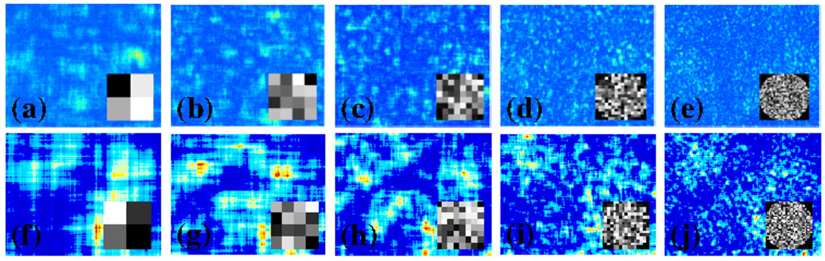
Figure 4.
Intensity cross-sections from the CCD using the graphite reflector performed both with and without pre-optimization. The SLM is divided into (a) segments, (b) segments, (c) segments and (d) segments.
Figure 4.
Intensity cross-sections from the CCD using the graphite reflector performed both with and without pre-optimization. The SLM is divided into (a) segments, (b) segments, (c) segments and (d) segments.
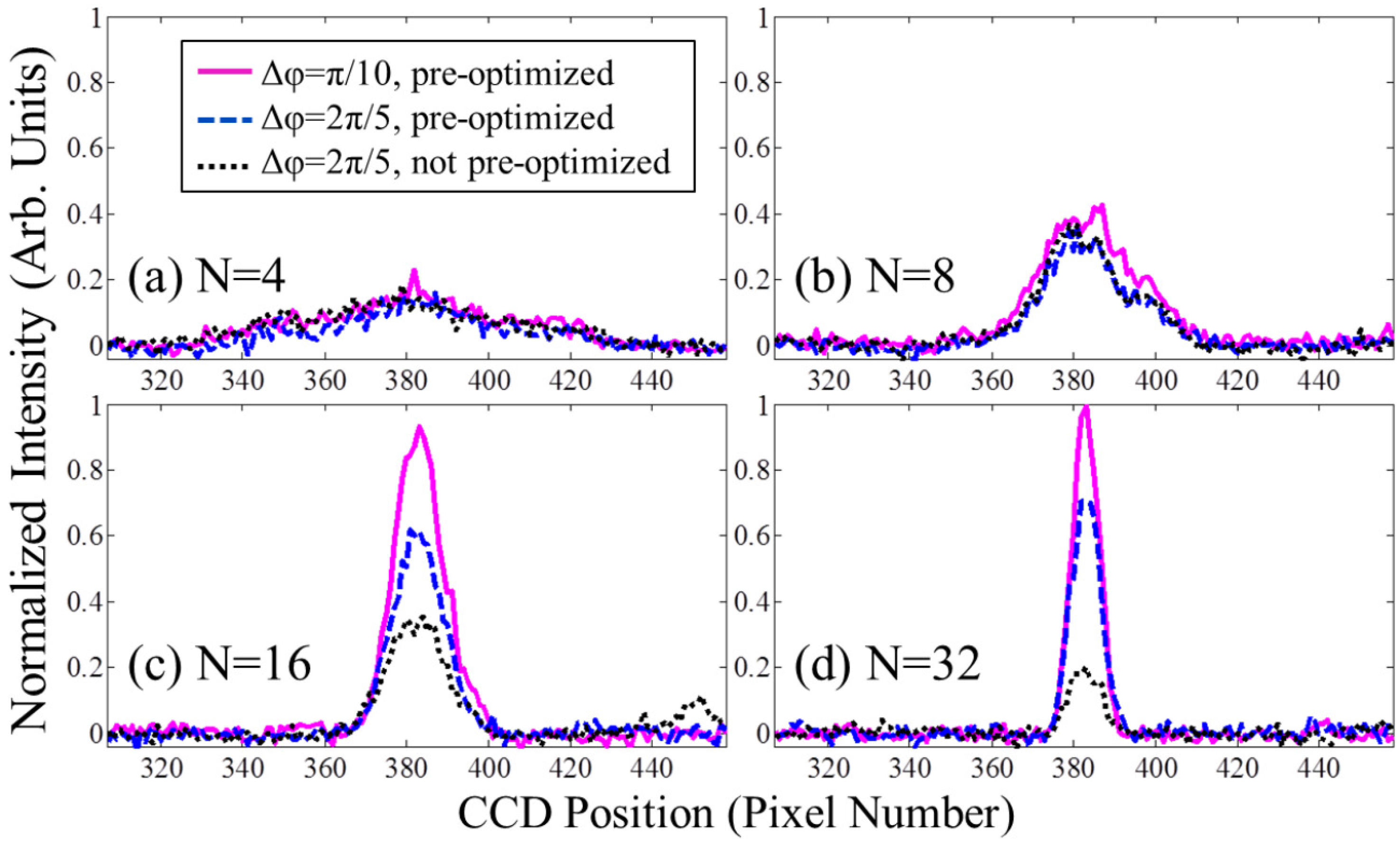
Figure 5.
The correlation coefficient of the speckle pattern produced by an unoptimized phase map as a function of time. Phase maps for and 32 are shown for the brushed aluminum, transmissive white paint on glass and Spectralon® samples.
Figure 5.
The correlation coefficient of the speckle pattern produced by an unoptimized phase map as a function of time. Phase maps for and 32 are shown for the brushed aluminum, transmissive white paint on glass and Spectralon® samples.

Figure 6.
Reflective inverse diffusion enhancement for each of the six reflector materials. The iterations are highlighted in gray. The iterations are highlighted in yellow.
Figure 6.
Reflective inverse diffusion enhancement for each of the six reflector materials. The iterations are highlighted in gray. The iterations are highlighted in yellow.

Figure 7.
Optimized reflective inverse diffusion spot intensities for the brushed aluminum reflector for through 32 (top) and corresponding intensity cross-sections (bottom).
Figure 7.
Optimized reflective inverse diffusion spot intensities for the brushed aluminum reflector for through 32 (top) and corresponding intensity cross-sections (bottom).

Figure 8.
Optimized spot intensities for transmissive inverse diffusion for the white paint on glass sample for through 32 (top) and corresponding intensity cross-sections (bottom). Background speckle size is relativity constant as N increases.
Figure 8.
Optimized spot intensities for transmissive inverse diffusion for the white paint on glass sample for through 32 (top) and corresponding intensity cross-sections (bottom). Background speckle size is relativity constant as N increases.

Figure 9.
The enhancement produced from a pre-optimized SLM for a given number of segments is plotted for computer simulations and experimental data for various reflector materials. Equation (10) is plotted (dotted-dashed line) for comparison.
Figure 9.
The enhancement produced from a pre-optimized SLM for a given number of segments is plotted for computer simulations and experimental data for various reflector materials. Equation (10) is plotted (dotted-dashed line) for comparison.
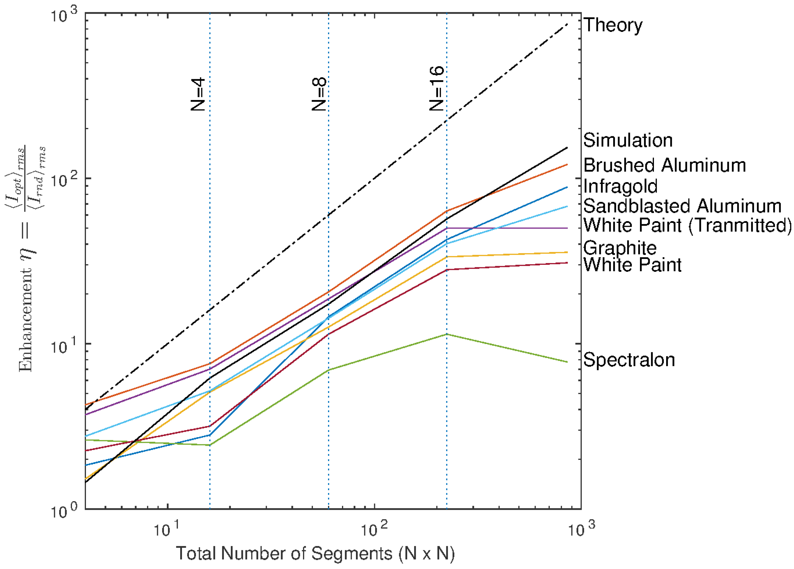
Figure 10.
Simulations of reflective inverse diffusion enhancement with zero-mean Gaussian distributed random phase fluctuations added to the reflector model. With the exception of , all reflector models are unimodular with a uniformly-distributed random phase. For , both the uniformly-distributed random phase model (red) and the circular Gaussian model (blue) are shown. The iterations are highlighted in gray. The iterations are highlighted in yellow.
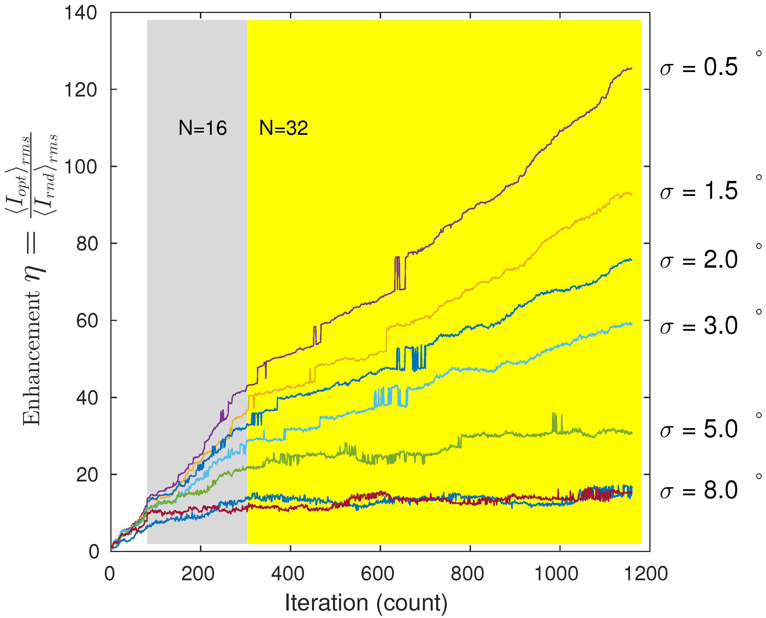
Figure 11.
Experimental distance definitions for spot size calculations.Spot Size

Figure 12.
Autocorrelation for each reflector from through . Red vertical lines mark the predicted spot size. The upper and lower bounds of the measured spot sizes are marked with vertical lines in cyan and magenta, respectively.
Figure 12.
Autocorrelation for each reflector from through . Red vertical lines mark the predicted spot size. The upper and lower bounds of the measured spot sizes are marked with vertical lines in cyan and magenta, respectively.

Figure 13.
Enhancement comparisons of specular and diffuse regions of reflection. Enhancement is plotted after each optimization with the CCD placed in the specular region at from the reflector surface normal (blue). Specular is defined as a reflection angle of from the surface normal. Diffuse is defined as off specular.


Table 1.
Summary values of enhancement, surface roughness and spot size for each of the six reflective samples measured and the one transmissive sample.
| Reflective Samples | Enhancement | Roughness | Final full width at half max (FWHM) |
|---|---|---|---|
| Brushed aluminum | 122.3 | 1.5 m | 36 ± 3 m |
| Infragold® | 89.9 | 9.4 m | 38 ± 3 m |
| Sandblasted aluminum | 67.7 | 2.3 m | 38 ± 3 m |
| Graphite | 37.3 | 3.5 m | 41 ± 3 m |
| White paint | 36.8 | 1.7 m | 41 ± 3 m |
| Spectralon® | 13.8 | Unprofiled | 45 ± 3 m |
| Transmissive Sample | |||
| White paint | 56.4 | 1.7 m | 63 ± 3 m |
© 2016 by the authors; licensee MDPI, Basel, Switzerland. This article is an open access article distributed under the terms and conditions of the Creative Commons Attribution (CC-BY) license (http://creativecommons.org/licenses/by/4.0/).
Share and Cite
MDPI and ACS Style
Burgi, K.; Ullom, J.; Marciniak, M.; Oxley, M. Reflective Inverse Diffusion. Appl. Sci. 2016, 6, 370. https://doi.org/10.3390/app6120370
AMA Style
Burgi K, Ullom J, Marciniak M, Oxley M. Reflective Inverse Diffusion. Applied Sciences. 2016; 6(12):370. https://doi.org/10.3390/app6120370
Chicago/Turabian StyleBurgi, Kenneth, Jessica Ullom, Michael Marciniak, and Mark Oxley. 2016. "Reflective Inverse Diffusion" Applied Sciences 6, no. 12: 370. https://doi.org/10.3390/app6120370
Note that from the first issue of 2016, this journal uses article numbers instead of page numbers. See further details here.