Wing Geometry and Kinematic Parameters Optimization of Flapping Wing Hovering Flight

Abstract

How to efficiently mimic the wing shape and kinematics pattern of an able hovering living flier is always a concern of researchers from the flapping wing micro aerial vehicles community. In this work, the separate or combined optimizations of wing geometry or/and wing kinematic parameters are systematically performed to minimize the energy of hovering flight, firstly on the basis of analytically extended quasi-steady aerodynamic model by using hybrid genetic algorithm. Before the elaboration of the optimization problem, the parametrization description of dynamically scaled wing with non-dimensional conformal feature of insect-scale rigid wing is firstly proposed. The optimization results show that the combined optimization of wing geometry and kinematic parameters can obtain lower flapping frequency, larger wing geometry parameters and lower power density in comparison with those from other cases of optimization. Moreover, the flapping angle for the optimization involving wing kinematic parameters manifests harmonic shape profile and the pitch angle possesses round trapezoidal profile with certain faster time scale of pitch reversal. The combined optimization framework provides a novel method for the conceptual design of fundamental parameters of biomimetic flapping wing micro aerial vehicle.

1. Introduction

The development of flapping wing micro aerial vehicles (FWMAV) has become a hot subject in the field of bio-inspired micro-devices engineering because its splendid properties, such as high maneuverability, portability and stealth with small characteristic size, are hopeful to be realized in near future [1,2,3,4,5]. However, it is far from sufficient to devise the most power-efficient schematic to build the FWMAV based on particular demand, e.g., carrying some certain mass of battery, avionics sensors and other payload to reach certain flight endurance and range [1]. For biomimetic design of FWMAV inspired by flying insects or hummingbirds, the critical starting point is to solve how to efficiently mimic the wing shape and kinematics pattern of the living flier, especially those who can maintain aloft hovering.

In the past decade, some attempts have been made to explore the optimal design space of wing geometry parameters (WGP) or wing kinematics parameters (WKP). Hedrick and Daniel explored the unconstrained WKP space controlling the hovering flight of hawkmoth through simulating the hovering dynamic ordinary differential equation based on quasi-steady aerodynamic model to be stabilized at a fixed position and orientation [6]. The optimization simulation that minimized the difference between the simulated and desired locations of the hawkmoth’s body in the global parameters space was performed by using the micro-genetic algorithm, which appended the Nelder-Mead simplex search algorithm, to find optimal WKP. Later, the sole optimization of WKP, which is reproduced by the neural network to form various function shapes of wing movements, was performed by Rakotomamonjy et al. to maximize the mean lift of the hovering FWMAV carrying available payload by using a simulation model called OSCAB (which stands for Outil de Simulation de Concept d’Ailes Battantes, French) and genetic algorithm (GA) [7]. Moreover, Berman and Wang conducted the sole optimization of wing kinematics pattern, which was characterized by specific functional forms determined by 11 parameters for three wing motion angles, to minimize the hovering power density of flapping wing insects on the basis of quasi-steady aerodynamic model by using hybrid-GA formed by the GA and Nelder–Mead simplex algorithm [8]. Subsequently, from the aspects of quasi-steady aerodynamic model and 2D computational fluid dynamics (CFD) numerical simulation separately, they performed a comparative study of aerodynamic efficiency between flapping wing hovering flight with optimal wing motions and fixed wing steady flight with optimal angle of attack under the constraint of lift balancing weight of fruit fly. They found that optimized flapping wing motions were more efficient than optimal steady flight [9,10]. Following the method of Berman and Wang, additionally considering the contribution of elastic strain energies to total mechanical energy, Kurdi et al. conducted similar study but used a different constrained nonlinear optimization solver to search for optimal wing kinematics formulated by spline interpolation [11]. The result shows that average mechanical power as a function of elastic storage decreased linearly with minimal benefits from the dissipation cost [11].

Recently, the higher order calculus of variation method was adopted by Taha et al. to minimize the aerodynamic power only on the basis of the translational aerodynamic analytical model under the constraint of lift with given WGP. After scrupulous analytical derivation, they found that a flapping angle featuring triangular waveform and pitch angle with constant value during a half-stroke could yield optimal aerodynamic performance [12]. Moreover, in order to acquire maximum lift or minimum power constrained by given lift, Nabawy and Crowther also studied the aero-optimum hovering wing kinematics only on the basis of translational aerodynamic analytical model. They found that flapping angle with sinusoidal profile and pitch angle with profile of rectangular wave could yield maximum lift with given flapping frequency and WGP, while flapping angle with profile of triangular shape and pitch angle also with rectangular profile could realize the minimization of power consumption with given lift constraint and WGP [13]. However, the effect of rotational circulation mechanism and added-mass effect on lift and power consumption has been neglected in their study. According to our best knowledge, these two aerodynamic mechanisms play an important role in wingbeat dynamics, especially in wing pitch motion’s realization and maintenance. Thus, they must be considered in the quasi-steady aerodynamic model and eventual power density model of flapping hovering flight.

It is noteworthy that an adjoint-based optimization method has been used to explore the combined optimization of wing shape and kinematics pattern of flapping wing hovering flight while maximizing the aerodynamic force coefficients [14]. The result shows that the highest improvement of aerodynamic performance could be obtained by optimal wing shape and kinematic parameters and there is an essential nonlinear dependence between them [14]. Although this method has provided a practical approach to optimize general unsteady aerodynamic flows and has the potential to perform highly efficient and discretely consistent sensitivity analysis for the any complicated problems [15,16], its successful realization is highly dependent on high-fidelity simulations for complicated model and calculation environments. And a wide range of research topics, such as the techniques of locally optimal, reduced-order model, and checkpointing used to reduce storage requirements, multi-fidelity optimization algorithms and convergence acceleration techniques that impact the computational cost, remain to be explored [16]. Moreover, some other methods, such as gradient-based method [17,18,19], sensitivity equations methods [20] and surrogated-based approach [21], also provide thinkable alternatives for optimization of wing shape and kinematics pattern of flapping wings flight. However, all of them suffer from excessive computational cost, which is directly proportional to the dimensionality of design variables. Several attempts based on experimental apparatus have also been made to perform the optimization of flapping-wing flows [22,23,24]. The deficiency of optimization based on the experiments is obvious, namely, the optimal results are limited by finite times of experiments and numbers of design variables.

Here, taking computational cost and dimensionality of design variables into consideration, we systematically performed the separate or combined optimizations of WGP or/and WKP to minimize the energy of hovering flight on the basis of extended quasi-steady aerodynamic model by using hybrid genetic algorithm (hybrid-GA) [8]. The essential nonlinear relationship between WGP and WKP via flow parameters (Re) is explored by minimization of the objective function, which is constructed by power density model with additional penalty items for lift-to-weight ratio, boundary constraints, linear constraint of aspect ratio (AR) and nonlinear constraint of Re. In this paper, two main highlights are presented. The first highlight is that the parametrization description of dynamically scaled wing with non-dimensional conformal feature of insect-scale rigid wing is firstly proposed. This parametrization method provides an effective simplifying way for aerodynamic analysis based on insect-scale rigid wings’ non-dimensional outline thus a feasibility of optimization involving WGP. The second highlight is that the combined optimizations of WGP and WKP are firstly performed to minimize the energy of flapping wing hovering flight on the basis of analytically extended quasi-steady aerodynamic model by using hybrid-GA. These two innovative points fill the research void of aerodynamic parameter’s combined optimization of flapping wing hovering energy minimization in analytical method.

The rest of this paper is organized as follows. Firstly, the parametrization characterization for dynamically scaled wing with non-dimensional conformal feature is developed in Section 2. Then the parametrization of wing kinematics pattern is prescribed in Section 3. In Section 4, we outline the extended quasi-steady aerodynamic model and present its verification and validation. The optimization problem is modeled and formulated in Section 5. The optimization results and the corresponding sensitivity analysis are given out in Section 6. Moreover, we make some discussion about the optimization results in Section 7. Lastly, we draw the conclusions in Section 8.

2. Wing Morphological Parametrization

The wing morphological parametrization is critical for the calculation of flapping wing aerodynamic, center of pressure (COP) and moments of inertia and thus for the determination of aerodynamic moment and efficiency. Here, due to the small size and lower inertial mass of the fruit fly wing planform and thus negligible deformation, we assume that the wing can be taken as a 2D rigid thin plate for simplifying analysis of inertial tensor and definition of wing kinematics [25,26]. The parametrization description of the wing shape for fruit fly, whose geometrical data has been measured by Muijres [27], is developed through further including the parametrization of the wing’s actual effective leading-edge profiles, the definition of wing pitch axis and the characterization of dynamically scaled wing with non-dimensional conformal feature.

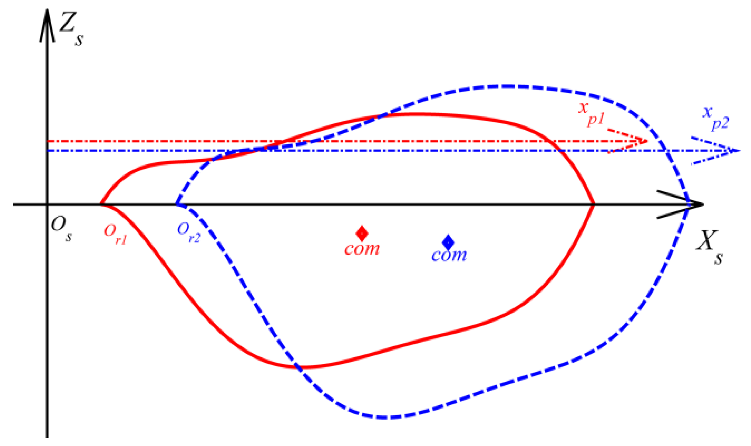
2.1. Description of Wing Morphology

The complete wing planform outline, wing shoulder frame (X_sO_sZ_s) and some basic sizes are illustrated in Figure 1. Here, the intersection of X_s-axis and Z_s-axis (O_s) can be termed wing shoulder [1,28], so we term the coordinate frame of X_sO_sZ_s as wing shoulder frame (or wing planform fixed frame). We assume that in the initial case, X_s-axis of X_sO_sZ_s is aligned with pitch axis, where r is the radial distance along it. It is worth noting that the wing hinge always exists in the insect body, so the wing root coordinate offset distance between wing shoulder (O_s) and wing root (O_r), which is commonly necessary to design the airfoil of FWMAV in engineering, is termed x_r,orig [29,30]. The variable pitch axis (x_p) is schemed by the red dash-dotted line. Here, $x_{0,\mathrm{vari}}$ denotes the projected distance between pitch-axis and maximum variable leading-edge point. As a starting point, we choose the X_s-axis of the wing shoulder frame as the original location of the pitch axis, which corresponds to the non-dimensional value of 0.36 from the maximum leading-edge point. In other words, the original leading-edge profiles ($z_{\mathrm{le},\mathrm{orig}}(r)$) and trailing-edge profiles ($z_{\mathrm{tr},\mathrm{orig}}(r)$) are prescribed in the wing shoulder frame firstly, then the value of 0.36 times the projected distance between maximum point on original leading-edge profiles and minimum point on original trailing-edge profiles relative to the original leading-edge profiles defines the initial pitch axis location, namely, z_le,orig,maxp/C_{max,letotr,orig} = 0.36 (Figure 1).

For conciseness of description, a statement is made that if there is no specific suffix on the right lower quadrant of some arguments, then the notation for this argument is possessed by the original or variable wing morphological parameters collectively, such as R_eff is possessed by R_eff,orig and R_eff,vari. In the wing shoulder frame, and chord length between leading-edge and trailing-edge profiles is C(r). Wing effective length (R_eff) is defined as the projected distance between the most proximal point (wing root) and the most distal point (wing tip) on the wing planform along the X_s-axis. Mean chord length (C_aver) is defined as the area of single wing (A_w) divided by wing effective length, A_w/R_eff (Table S1). The actual original wing outline of leading-edge ($z_{\mathrm{le},\mathrm{orig}}(r)$) and trail-edge ($z_{\mathrm{tr},\mathrm{orig}}(r)$) for fruit fly has been obtained through polynomial fitting the geometrical data located in the coordinate frame of X_sO_sZ_s (Figure 1 and Tables S2 in the Supplementary Materials). The geometrical data of the wing is transposed and translated from the original right wing geometrical data measured by Muijres [27].

2.2. Non-Dimensional Parametrization of Wing Morphology

Following the non-dimensional way of Ellington [31], we write the wing morphology in non-dimensional form by applying wing effective length (R_eff) and mean chord (C_aver) as the length scale for size parameter components along X_s-axis and Z_s-axis, respectively. A series of non-dimensional parameters has been acquired, for example, non-dimensional x-root offset ${\widehat{x}}_r$ = x_r/R_eff, non-dimensional radial distance $\widehat{r}$ = r/R_eff, non-dimensional leading-edge profiles ${\widehat{z}}_{\mathrm{le}}(\widehat{r})=z_{\mathrm{le}}(r)/C_{\mathrm{aver}}$, non-dimensional trailing-edge profiles ${\widehat{z}}_{\mathrm{tr}}(\widehat{r})=z_{\mathrm{tr}}(r)/C_{\mathrm{aver}}$, and non-dimensional chord distribution $\widehat{C}(\widehat{r})=C(r)/C_{\mathrm{aver}}$. Here, aspect ratio (AR) is equal to R_eff/C_aver for the single wing planform. Eventually, the parameters of wing planform can be determined by wing effective length (R_eff), mean chord (C_aver), non-dimensional leading-edge and trailing-edge profiles (${\widehat{z}}_{\mathrm{le}}(\widehat{r})$ and ${\widehat{z}}_{\mathrm{tr}}(\widehat{r})$).

2.3. Characterization of Dynamically Scaled Wing

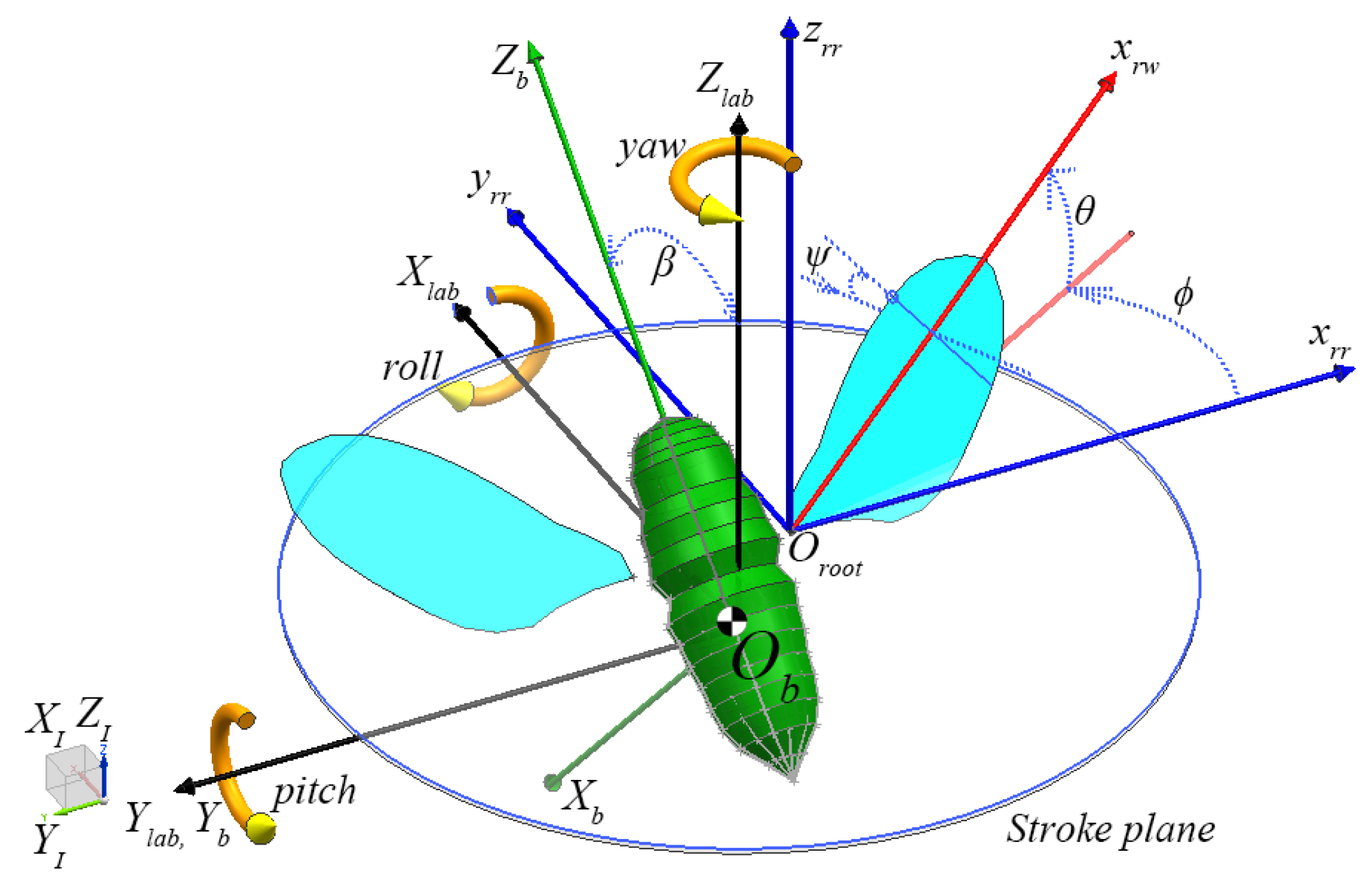
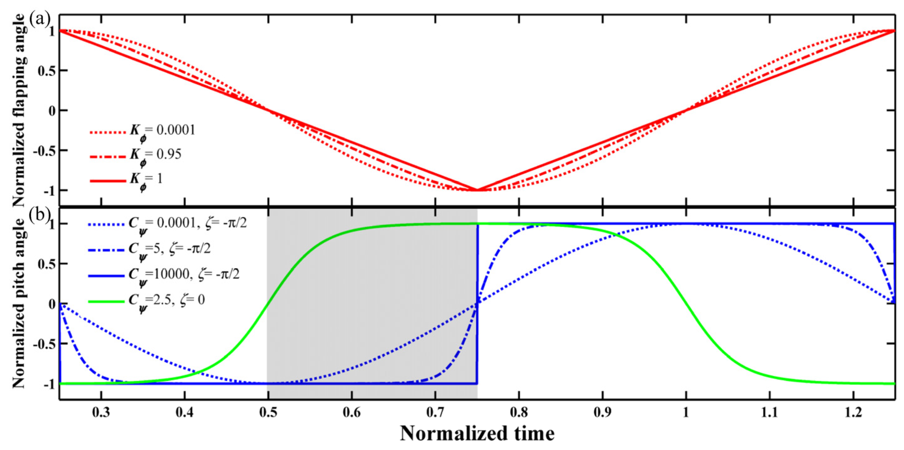
The posterior optimization problem involving WGP firstly needs the characterization of non-dimensional parameters and mass properties of dynamically scaled wing planform. In the current study, non-dimensional leading-edge (${\widehat{z}}_{\mathrm{le}}\left(\widehat{r}\right)$), and non-dimensional trailing-edge profiles (${\widehat{z}}_{\mathrm{tr}}\left(\widehat{r}\right)$), which are from the geometry outlines of fruit fly, are assumed to remain unchanged. The variable wing effective length ($R_{\mathrm{eff},\mathrm{vari}}$) and variable mean chord ($C_{\mathrm{aver},\mathrm{vari}}$) are chosen to regulate the dynamically scaled wing planform outlines. Moreover, the variable x-root offset ($x_{\mathrm{r},\mathrm{vari}}$) and variable non-dimensional pitch axis location relative to the maximum point of actual leading-edge profile (${\widehat{x}}_{0,\mathrm{vari}}$) are adopted to regulate the aerodynamic performance of the dynamically scaled wing planform. The distance of the wing root and shoulder ($x_{r,\mathrm{vari}}$) in engineering design is always arbitrarily determined only according to the assembly gap between transmission of drivetrain and overlap joint of the wing planform. This determining way neglects its effect on aerodynamic characteristics of hovering wing planform due to the fact that a constant velocity contribution from the interval of wing shoulder and root is added to linearly varying velocity of the whole wing planform [29,30]. While the non-dimensional pitch axis location (${\widehat{x}}_{0,\mathrm{vari}}$) of the dynamically scaled fruit fly wing model shall influence the experimental rotational coefficient [32]. So it is necessary to choose the x-root offset and non-dimensional rotational axis location as two additional variables to complete the optimized parameters’ characterization of the dynamically scaled wing planform.

The mass properties for the dynamically scaled wing planform are prepared for the optimization involving WGP by assuming that the wing mass was uniform isotropic distribution with very small thickness. Firstly, a three-dimensional (3D) geometry model is constructed from the original wing geometry data by CAD software (UGS NX 7.5, siemens plm software, Plano, TX, USA). The mass of wing ($m_{\mathrm{wing},\mathrm{orig}}$), center of mass (COM) in the frame of X_sO_sZ_s ($x_{\mathrm{com},\mathrm{orig}}$ and $z_{\mathrm{com},\mathrm{orig}}$), and moment of inertia relative to the COM ($I_{xx,\mathrm{com},\mathrm{orig}}$ and $I_{zz,\mathrm{com},\mathrm{orig}}$) are calculated and listed in Table S1. Then, two ratios between dynamically scaled wing planform and original wing planform of the fruit fly are developed. They are wing length ratio ($R_{\mathrm{ratio}}$) between variable wing effective length ($R_{\mathrm{eff},\mathrm{vari}}$) and original wing effective length ($R_{\mathrm{eff},\mathrm{orig}}$), and mean chord ratio ($C_{\mathrm{ratio}}$) between variable mean chord length ($C_{\mathrm{aver},\mathrm{vari}}$) and original mean chord length ($C_{\mathrm{aver},\mathrm{orig}}$), respectively. It is not difficult to find the relation of COM in the frame of X_sO_sZ_s for the wing planform before and after it is dynamically changed (as seen in Figure 2, the variable pitch axis (x_pi) are also illustrated). The calculating formulation for COM of the dynamically changed wing planform with non-dimensional conformal feature in the frame of X_sO_sZ_s can be expressed as:

$$x_{\mathrm{com},\mathrm{vari}}=R_{\mathrm{ratio}}(x_{\mathrm{com},\mathrm{orig}}-x_{\mathrm{r},\mathrm{orig}})+x_{\mathrm{r},\mathrm{vari}},$$

(1)

$$z_{\mathrm{com},\mathrm{vari}}=C_{\mathrm{ratio}}{z}_{\mathrm{com},\mathrm{orig}}.$$

(2)

The dynamically changed wing planform’s mass has the form of $m_{\mathrm{wing},\mathrm{vari}}=R_{\mathrm{ratio}}{C}_{\mathrm{ratio}}{m}_{\mathrm{wing},\mathrm{orig}}$. Thirdly, according to the definition formulation of inertial tensor [25], the moment of inertia of the dynamically scaled wing planform relative to the changed COM can be expressed as:

$$I_{xx,\mathrm{com},\mathrm{vari}}=R_{\mathrm{ratio}}{C_{\mathrm{ratio}}}^3{I}_{xx,\mathrm{com},\mathrm{orig}},$$

(3)

$$I_{zz,\mathrm{com},\mathrm{vari}}={R_{\mathrm{ratio}}}^3{C}_{\mathrm{ratio}}{I}_{zz,\mathrm{com},\mathrm{orig}}.$$

(4)

So the moment of inertia of the dynamically scaled wing planform in the frame of X_sO_sZ_s can be acquired through generalized parallel-axis theorem:

$$I_{xx,\mathrm{vari}}=I_{xx,\mathrm{com},\mathrm{vari}}+m_{\mathrm{wing},\mathrm{vari}}{z_{\mathrm{com},\mathrm{vari}}}^2,$$

(5)

$$I_{zz,\mathrm{vari}}=I_{zz,\mathrm{com},\mathrm{vari}}+m_{\mathrm{wing},\mathrm{vari}}{x_{\mathrm{com},\mathrm{vari}}}^2.$$

(6)

Thus, the complete optimized parameters characterization for the dynamically scaled fruit fly wing planform has been finished. It is worth noting that this parametrization description of dynamically scaled wing with non-dimensional conformal feature is not limited to the wing morphology of the fruit fly but also applicable to some symmetric or asymmetric and regular or irregular wing planforms [29]. The aerodynamic characteristics comparisons of these wing planforms with different wing leading and trailing edge outlines go beyond the scope of this work.

3. Wing Kinematics

In this paper, the right wing Euler angles relative to stroke plane in right wing root frame of reference ($x_{rr}{y}_{rr}{z}_{rr}$) are defined by three angles (flapping angle (ϕ), stroke deviation angle (θ) and pitch angle (ψ), Figure 3). The determination of direction of three angles obeys a right-hand rule. Moreover, the body frame of reference (X_bY_bZ_b) and lab frame of reference (X_labY_labZ_lab) for fruit fly are also illustrated for clarity. The stroke plane is the horizontal plane of the lab frame of reference (X_labO_bZ_lab). The radius vector of O_root relative to O_b is neglected in posterior torques calculation. The inclined angle of longitudinal body axis (Z_b) relative to Z_lab axis (β) is 47.5° for hovering fruit fly [27]. Take a concise hovering design and simplifying optimization analysis for FWMAV in engineering into consideration [2,12,33], we assume the stoke deviation is absent. Using the coordination systems shown in Figure 3, we write the complete transformation matrix from the right wing root frame of reference ($x_{rr}{y}_{rr}{z}_{rr}$) to the right wing planform fixed frame ($x_{rw}{y}_{rw}{z}_{rw}$) as

$${}_{rr}{}^{rw}R=\left[\begin{array}{ccc}\cos \varphi & \sin \varphi & 0\\ -\cos \psi \sin \varphi & \cos \psi \cos \varphi & \sin \psi \\ \sin \psi \sin \varphi & \sin \psi \cos \varphi & \cos \psi \end{array}\right].$$

(7)

The converse transformation matrix from the wing planform fixed frame to the right wing root frame of reference can be given by ${}_{rw}{}^{rr}R={}_{rr}{}^{rw}R^{-1}$. According to above transformation and wing kinematics differentiating to time, the wing angular velocity vector in right wing planform fixed frame can be acquired from the transformation of the middle coordination frame (mid) to the right wing planform fixed frame due to flapping and pitch motion, namely, ${}^{rw}\omega ={}_{mid}{}^{rw}R_{x,-\psi }\dot{\varphi }\overrightarrow{k_{mid}}+\dot{\psi }\overrightarrow{i_{rw}}$, where i and k denote unit vectors along x and z directions of local frame, respectively, and the right superscript of ${}^{rw}\omega$ is the abbreviation of the right wing. Thus ${}^{rw}\omega$ can be extended as

$${}^{rw}\omega =\left[\begin{array}{c}{\omega }_x\\ {\omega }_y\\ {\omega }_z\end{array}\right]=\left[\begin{array}{ccc}1& 0& 0\\ 0& \cos \psi & \sin \psi \\ 0& -\sin \psi & \cos \psi \end{array}\right]\left[\begin{array}{c}0\\ 0\\ \dot{\varphi }\end{array}\right]+\left[\begin{array}{c}\dot{\psi }\\ 0\\ 0\end{array}\right]=\left[\begin{array}{c}\dot{\psi }\\ \dot{\varphi }\sin \psi \\ \dot{\varphi }\cos \psi \end{array}\right],$$

(8)

where the left superscript of ${}^{rw}\omega$ is the abbreviation of the right wing. The wing angular acceleration velocity vector ${}^{rw}\dot{\omega }$ in the right wing planform fixed frame can be expressed as

$${}^{rw}\dot{\omega }=\left[\begin{array}{c}{\dot{\omega }}_x\\ {\dot{\omega }}_y\\ {\dot{\omega }}_z\end{array}\right]=\left[\begin{array}{c}\ddot{\psi }\\ \ddot{\varphi }\sin \psi +\dot{\varphi }\dot{\psi }\cos \psi \\ \ddot{\varphi }\cos \psi -\dot{\varphi }\dot{\psi }\sin \psi \end{array}\right].$$

(9)

Here, in order to additionally consider the effect of time scale of wing stroke reversal and wing pitch reversal on optimization including WKP, we adopt the wing kinematic pattern of Berman and Wang [8], but overlook the effect of stroke plane deviation angle on optimization because of its low amptitude [12,21].

$$\varphi (t)=\frac{{\varphi }_m}{{\sin }^{-1}\left(K_{\varphi }\right)}{\sin }^{-1}\left(K_{\varphi }\sin \left(2\pi ft\right)\right),$$

(10)

$$\psi (t)=\frac{{\psi }_m}{\tanh C_{\psi }}\tanh \left[C_{\psi }\sin \left(2\pi ft+\zeta \right)\right],$$

(11)

where ϕ(t) is flapping angle, ψ(t) is pitch angle (Figure 3). ϕ_m and ψ_m are flapping and pitch angle amplitude, respectively. Their boundary values are listed in

Table 1. Independent variable wing geometry parameters (WGP) and wing kinematics parameters (WKP) and their constraints.

Variables	Description	Min	Max
Reff,vari (mm)	wing effective length	2	4 a
Caver,vari (mm)	mean chord length	0.5	2 a
xr,vari (mm)	x-root offset	0	2 a
${\widehat{x}}_0$	rotational axis location	0	0.36
f (Hz)	Frequency	0	∞
ϕm (rad)	Flapping amplitude	0	1.309
Kϕ	Regulating parameters of flapping angle profiles	0	1
ψm (rad)	Pitch amplitude	0	π/2
ζ (rad)	Pitch phase offset	−π/2	0
Cψ	Regulating parameters of pitch angle profiles	0	5

^a prescribed by referring to the constraints of AR in Section 5.2.

in terms of empirically observed value (ϕ_m = 75°) and suggested value (ψ_m = π/2) [8]. K_ϕ and C_ψ are regulating parameters of profiles of flapping and pitch angle, respectively. The bound of K_ϕ is listed in Table 1 according to the reported values [8]. While the bound of C_ψ is limited in the range from 0 to 5 by referring to the upper bound suggested by Nabawy and Crowther [13,30]. It is necessary to limit the upper bound of C_ψ at a relative value of 5, which means that the pitch reversal of the wing should be completed within around 25% of the stroke period. The larger the upper bound of C_ψ, the shorter the pitch reversal complete, then the pitch acceleration during pitch reversal shall be more larger, which must induce extremely large inertia force, including inertia force of wing planform itself and added-mass force derived from the inviscid irrotational model [25]. This is not in agreement with the practical physical situation of flapping wing hovering aerodynamic force. Thus the upper bound of C_ψ must be limited at a reasonable value [13,30]. As shown in Figure 4, the profiles of flapping angle and pitch angle separately change from harmonic to triangular and round trapezoidal waveform with K_ϕ and C_ψ varying from their lower boundaries to upper boundaries (Table 1). ζ is the phase offset of the pitch angle relative to the flapping angle. Here, we define ψ = 0° when the wing planform is vertical to the horizontal stroke plane, thus the pitching offset (η₀) in the wing kinematic pattern of Berman and Wang can be discarded [8]. According to the probable passivity of wing pitch dynamic or observed results for nearly all insects that the leading edge of wing planform is always above wing stroke plane [8], we limit the range of phase offset (ζ) within −π/2 to 0 (Figure 4 and Table 1).

Thus, a two degrees of freedom (DOF) wing kinematic pattern is parameterized by six variables. The other independent variables and their constraint boundaries are listed in Table 1.

4. Extended Quasi-Steady Aerodynamic Model

Here, we assume that flapping wing fruit fly can always keep hovering in flight, so the revised quasi-steady aerodynamic model can be adopted to estimate the aerodynamic force of the flapping wing thin plate passing through unsteady flow [32,34,35]. Considering the assumption and applicability of revised quasi-steady aerodynamic model, a nonlinear constraint for posterior optimization analysis of minimum energy is defined via Reynolds number, Re = U_averC_aver/ν. Here U_aver is mean translating velocity of wing tip expressed as 4ϕ_mfR_eff, and ν is kinematic viscosity of air (1.48 × 10⁻⁵ m²/s). The hovering flight of flapping wing insects including fruit fly usually has a low Re approximate to 100~3000 [25,36,37], in which range the quasi-steady aerodynamic model has been proved to be able to estimate experimental result very well [32,35]. Here, we shall derive aerodynamic forces and moments component analytical formulas for three aerodynamic mechanisms, namely, translational and rotational circulation mechanism and added mass effect. It is worth noting that the aerodynamic damping moment, which plays an important role in realizing smooth pitch rotation of wing planform [25], is introduced into the pitch-axis aerodynamic moment. Moreover, the aerodynamic damping moment that stems from the velocity gradient of each strip along chordwise differential elements due to pitch motion of wing planform [8,25,38,39,40] is also included to complete the development of aerodynamic moments. Thus, the current aerodynamic model can be termed an extended version of quasi-steady aerodynamic model.

4.1. Aerodynamic Forces

As seen in Figure 1, the blade-element method assumes that the aerodynamic force acting on the wing planform is the summation of force acting on each infinitesimal spanwise strip, and the local pressure drag acting on each strip is the summation of normal pressure drag acting on the chordwise differential elements. So the aerodynamic forces in the wing planform fixed frame, which are produced by translational circulation, rotational circulation, and added mass effect, can be given by

$$F_{\mathrm{trans},y}=\frac{1}{2}\rho {R_{\mathrm{eff},\mathrm{vari}}}^3{C}_{\mathrm{aver},\mathrm{vari}}{\widehat{F}}_{\mathrm{trans}}{C}_{\mathrm{N}}\left(\alpha \right){{\omega }_{\mathrm{pal}}}^2,$$

(12)

$$F_{\mathrm{rot},y}=\frac{1}{2}\rho {R_{\mathrm{eff},\mathrm{vari}}}^2{C_{\mathrm{aver},\mathrm{vari}}}^2{\widehat{F}}_{\mathrm{rot}}{C}_{\mathrm{R}}{\omega }_x{\omega }_{\mathrm{pal}},$$

(13)

$$F_{\mathrm{add},y}=\frac{\pi }{4}\rho {C_{\mathrm{aver},\mathrm{vari}}}^2{R_{\mathrm{eff},\mathrm{vari}}}^2{\widehat{F}}_{\mathrm{rot}}\left({\dot{\omega }}_z+{\omega }_x{\omega }_y\right)+\frac{\pi }{4}\rho {C_{\mathrm{aver},\mathrm{vari}}}^3{R}_{\mathrm{eff},\mathrm{vari}}{\widehat{F}}_{\mathrm{coeff},\mathrm{add},y}{\dot{\omega }}_x,$$

(14)

where ${\widehat{F}}_{\mathrm{trans}}$ and ${\widehat{F}}_{\mathrm{rot}}$ can be termed non-dimensional translational and rotational aerodynamic force, respectively [25]. And ${\widehat{F}}_{\mathrm{coeff},\mathrm{add},y}$ can be analogously termed non-dimensional rotational added-mass aerodynamic coefficient. Their complete expression is detailed in

Table 2. Non-dimensional aerodynamic parameters for different aerodynamic components.

Aerodynamic Components	Abbreviation	Calculation Formulas
Translational components	${\widehat{F}}_{\mathrm{trans}}$	${\widehat{F}}_{\mathrm{trans}}={\displaystyle {\int }_0^1{\left(\widehat{r}+{\widehat{x}}_{\mathrm{r},\mathrm{vari}}\right)}^2\widehat{C}\left(\widehat{r}\right)\mathrm{d}\widehat{r}}$
	${\widehat{M}}_{\mathrm{coeff},\mathrm{trans},z}$	${\widehat{M}}_{\mathrm{coeff},\mathrm{trans},z}={\displaystyle {\int }_0^1{\left(\widehat{r}+{\widehat{x}}_{\mathrm{r},\mathrm{vari}}\right)}^3\widehat{C}\left(\widehat{r}\right)\mathrm{d}\widehat{r}}$
	${\widehat{r}}_{\mathrm{spw},\mathrm{cop},\mathrm{trans}}$	${\widehat{r}}_{\mathrm{spw},\mathrm{cop},\mathrm{trans}}=\frac{{\widehat{M}}_{\mathrm{coeff},\mathrm{trans},z}}{{\widehat{F}}_{\mathrm{trans}}}$
Rotational components	${\widehat{F}}_{\mathrm{rot}}$	${\widehat{F}}_{\mathrm{rot}}={\displaystyle {\int }_0^1\left(\widehat{r}+{\widehat{x}}_{\mathrm{r},\mathrm{vari}}\right)\widehat{C}{\left(\widehat{r}\right)}^2\mathrm{d}\widehat{r}}$
	${\widehat{M}}_{\mathrm{coeff},\mathrm{rot},z}$	${\widehat{M}}_{\mathrm{coeff},\mathrm{rot},z}={\displaystyle {\int }_0^1{\left(\widehat{r}+{\widehat{x}}_{\mathrm{r},\mathrm{vari}}\right)}^2\widehat{C}{\left(\widehat{r}\right)}^2\mathrm{d}\widehat{r}}$
	${\widehat{r}}_{\mathrm{spw},\mathrm{cop},\mathrm{rot}}$	${\widehat{r}}_{\mathrm{spw},\mathrm{cop},\mathrm{rot}}=\frac{{\widehat{M}}_{\mathrm{coeff},\mathrm{rot},z}}{{\widehat{F}}_{\mathrm{rot}}}$
Aerodynamic damping components	${\widehat{M}}_{\mathrm{coeff},\mathrm{rd},x}$	${\widehat{M}}_{\mathrm{coeff},\mathrm{rd},x}={\displaystyle {\int }_0^1{\widehat{z}}_{\mathrm{rd}}\left(\widehat{r}\right)\mathrm{d}\widehat{r}}$ a
	${\widehat{M}}_{\mathrm{coeff},\mathrm{rd},z}$	${\widehat{M}}_{\mathrm{coeff},\mathrm{rd},z}={\displaystyle {\int }_0^1\widehat{C}{\left(\widehat{r}\right)}^3\left({\widehat{x}}_{\mathrm{r},\mathrm{vari}}+\widehat{r}\right)\mathrm{d}\widehat{r}}$
Added-mass components	${\widehat{F}}_{\mathrm{coeff},\mathrm{add},y}$	${\widehat{F}}_{\mathrm{coeff},\mathrm{add},y}={\displaystyle {\int }_0^1\widehat{C}{\left(\widehat{r}\right)}^2}{\widehat{z}}_{\mathrm{h}}\mathrm{d}\widehat{r}$ b
	${\widehat{M}}_{\mathrm{coeff},\mathrm{add},z,1}$	${\widehat{M}}_{\mathrm{coeff},\mathrm{add},z,1}={\displaystyle {\int }_0^1\widehat{C}{\left(\widehat{r}\right)}^2{\left(\widehat{r}+{\widehat{x}}_{\mathrm{r},\mathrm{vari}}\right)}^2\mathrm{d}\widehat{r}}$
	${\widehat{I}}_{xx,\mathrm{am}}$	${\widehat{I}}_{xx,\mathrm{am}}={\displaystyle {\int }_0^1\widehat{C}{\left(\widehat{r}\right)}^2}\left({\widehat{z}}_{\mathrm{h}}{\left(\widehat{r}\right)}^2+\frac{1}{32}\widehat{C}{\left(\widehat{r}\right)}^2\right)\mathrm{d}\widehat{r}$ b
	${\widehat{I}}_{xz,\mathrm{am}}$	${\widehat{I}}_{xz,\mathrm{am}}={\displaystyle {\int }_0^1\left(\widehat{r}+{\widehat{x}}_{\mathrm{r},\mathrm{vari}}\right)}\widehat{C}{\left(\widehat{r}\right)}^2{\widehat{z}}_{\mathrm{h}}\left(\widehat{r}\right)\mathrm{d}\widehat{r}$ b

^a ${\widehat{z}}_{\mathrm{rd}}\left(\widehat{r}\right)=\frac{1}{4}\left[\left|{\widehat{z}}_{\mathrm{le},\mathrm{orig}}\left(\widehat{r}\right)-\widehat{\Delta }\right|{\left({\widehat{z}}_{\mathrm{le},\mathrm{orig}}\left(\widehat{r}\right)-\widehat{\Delta }\right)}^3-\left|{\widehat{z}}_{\mathrm{le},\mathrm{orig}}\left(\widehat{r}\right)-\widehat{\Delta }-\widehat{C}\left(\widehat{r}\right)\right|{\left({\widehat{z}}_{\mathrm{le},\mathrm{orig}}\left(\widehat{r}\right)-\widehat{\Delta }-\widehat{C}\left(\widehat{r}\right)\right)}^3\right]$; ^b ${\widehat{z}}_{\mathrm{h}}\left(\widehat{r}\right)=\frac{1}{2}\widehat{C}\left(\widehat{r}\right)-\left({\widehat{z}}_{\mathrm{le},\mathrm{orig}}\left(\widehat{r}\right)-\widehat{\Delta }\right)$.

. $C_{\mathrm{R}}$ is the theoretical rotational coefficient with expression of $C_{\mathrm{R}}=\pi (0.75-{\widehat{x}}_{0,\mathrm{vari}})$, and ${\omega }_{\mathrm{pal}}$, which is equal to $\dot{\varphi }$, is defined as the angular velocity of the pitch axis line of wing planform. Here, for translational aerodynamic force, its tangential component is neglected due to its small contribution [30,41,42]. The normal translational aerodynamic force coefficient ($C_{\mathrm{N}}\left(\alpha \right)$, α is angle of attack) is obtained from lift and drag coefficients using trigonometry. Within the community of the flapping wing, the two-dimensional (2D) quasi-static lift and drag coefficients in the local flow for translational circulation mechanism adopted broadly are from simple harmonic fitness relationships to the experimental data for the dynamically scaled fruit fly wing model [34],

$$\{\begin{array}{c}{C}_{\mathrm{L}}\left(\alpha \right)=0.225+1.58\sin \left(2.13\alpha -7.2\right)\\ C_{\mathrm{D}}\left(\alpha \right)=1.92-1.55\cos \left(2.04\alpha -9.82\right)\end{array},$$

(15)

These formulas might be appropriately used to evaluate translational component of aerodynamic force for dynamically scaled wing planform with non-dimensional conformal feature. However, the translational aerodynamic lift and drag coefficients for prolonged attachment of the leading edge vortex (LEV) might be influenced by the variation of wing shape. As concluded and remarked by Birch and Dickinson [43], the prolonged attachment of LEV on insect-scale wings may be due to the attenuating effect of downwash induced by the tip vortex and wake vorticity but not spanwise flow under lower Re for fruit flies, such as 100 ± 250. Thus, it is necessary to try to analytically explore whether the variation of wing shape will indirectly have much influence on lift and power density by probable way of influencing translational aerodynamic coefficients.

In order to account for the possible effect of any variation of wing shape on aerodynamic coefficients thus lift and power, an approximate expression to experimental data for translational steady lift coefficient is also utilized to model the lift for flapping wing biomechanics of insect or FWMAV [30,44], this expression for 3D translational lift coefficient is given by

$$C_{\mathrm{L}}\left(\alpha \right)=0.5C_{L\alpha }\sin \left(2\alpha \right),$$

(16)

where C_Lα is 3D wing lift curve slope. Recently, Taha and Nabawy give out 3D lift curve slope based on Extended Lifting Line Theory and Prandtl lifting line theory, respectively [30,44]. Here, the 3D lift curve slope given by Nabawy is adopted because it takes care of some correction for unsteady aerodynamic mechanism through edge correction except aspect ratio. According to the Prandtl lifting line theory [30], the 3D wing lift curve slope ($C_{L\alpha }$) for aspect ratio above 3 can be given by

$$C_{L\alpha }=\frac{C_{L\alpha ,2d}}{E_{\mathrm{vari},ec}+k{C}_{L\alpha ,2d}/\pi A{R}_{\mathrm{vari}}},$$

(17)

where C_La,2d is 2D aerofoil lift curve for a flat plate. The value of 0.09 deg⁻¹ is adopted for rigid thin wing planform at typical insect wing’s Re [30]. The variable aspect ratio, AR_vari, is equal to R_eff,vari/C_aver,vari for a single wing. The parameter k, which can be evaluated by induced power factor according to a hovering actuator disc model [30], is termed ‘k-factor’. The k-factor for the normal hovering flight of a fruit fly can take the value of 1.51 in terms of the estimating result of Nabawy and Crowther through including three contributors of the non-uniform downwash velocity distribution, tip losses and effective flapping disc area [30]. The parameter, E_vari,ec, is edge correction based on lifting line theory considering the 3D effect of variation of wing shape [30]. Accounting for simplification in the integral of wing planform semi-perimeter, we assume that the edge correction (E_vari,ec) for dynamically scaled wing planform can be estimated as

$$E_{vari,ec}={\lambda }_1{R}_{\mathrm{ratio}}{C}_{\mathrm{ratio}}{E}_{\mathrm{orig},\mathrm{ec}},$$

(18)

where a factor of shape, λ₁, is introduced to match 3D lift coefficient of original wing planform to 2D quasi-static lift coefficient fitted from experimental data for dynamically scaled fruit fly wing model [34] (Figure 5). A value of 0.62 is used with root-mean-squared error (RMSE) of 0.04 relative to 2D quasi-static data. The edge correction for the original wing planform, E_orig,ec, is calculated by the quotient of the wing semi-perimeter to its length [33], as given by

$$E_{\mathrm{orig},\mathrm{ec}}=\frac{C_{\mathrm{semi},\mathrm{perim}}}{R_{\mathrm{eff},\mathrm{vari}}},$$

(19)

here, $C_{\mathrm{semi},\mathrm{perim}}=\frac{S_{\mathrm{le},\mathrm{orig}}+S_{\mathrm{tr},\mathrm{orig}}}{2}$ is semi-perimeter of original fruit fly wing planform. The arc length of leading-edge and trailing edge profiles can be expressed as

$$S_{i,\mathrm{orig}}={\displaystyle {\int }_{x_{r,\mathrm{orig}}}^{R_{\mathrm{eff},\mathrm{orig}}}{\left(1+{\left(\frac{d{z}_{i,\mathrm{orig}}\left(r\right)}{dr}\right)}^2\right)}^{\frac{1}{2}}dr},$$

(20)

where i ($i=\mathrm{le},\mathrm{tr}$) denotes leading-edge and trailing edge profiles.

Once the 3D translational lift coefficient is obtained, the drag coefficient can be obtained by using trigonometry:

$$C_{\mathrm{D}}\left(\alpha \right)={\lambda }_2{C}_{\mathrm{L}}\left(\alpha \right)\tan \left(\alpha \right)={\lambda }_2{C}_{\mathrm{L}}\left(\alpha \right){\sin }^2\left(\alpha \right),$$

(21)

Similarly, a factor of shape, λ₂, is introduced to match 3D drag coefficient of original wing planform to 2D quasi-static drag coefficient (Figure 5). A value of 0.93 is used with RMSE of 0.11 relative to 2D quasi-static data. As shown in Figure 5, the 3D lift and drag coefficients of (16) and (21) have a good approximation with the fitting formulas based on experimental data with little RMSE after introduced two factors of shape. Thus these formulas of translational lift and drag coefficients constructed by 3D lift curve slope based on Prandtl lifting line theory [30] are also adopted for comparing the possible effect of wing aerodynamic performance arising from variation of wing shape on optimization involving WGP. Finally, the normal translational aerodynamic force coefficient can be obtained by a simple transformation, C_N (α) = cos(α)C_L(α) + sin(α)C_D(α).

4.2. Aerodynamic Moments

The aerodynamic moments in wing planform fixed frame, which are produced by the mechanisms of translational circulation, rotational circulation, aerodynamic damping moment, and added mass effect, can be expressed as

$$M_{\mathrm{trans},z}=\frac{1}{2}\rho {R_{\mathrm{eff},\mathrm{vari}}}^4{C}_{\mathrm{aver},\mathrm{vari}}{\widehat{M}}_{\mathrm{coeff},\mathrm{trans},z}{C}_{\mathrm{N}}\left(\alpha \right){{\omega }_{\mathrm{pal}}}^2{\overrightarrow{e}}_z,$$

(22)

$$M_{\mathrm{trans},x}=\frac{1}{2}\rho {R_{\mathrm{eff},\mathrm{vari}}}^3{C_{\mathrm{aver},\mathrm{vari}}}^2{\widehat{F}}_{\mathrm{trans}}{\widehat{Z}}_{\mathrm{cop},\mathrm{trans}}\left(\alpha \right)C_{\mathrm{N}}\left(\alpha \right){{\mathsf{\omega }}_{\mathrm{pal}}}^2,$$

(23)

$$M_{\mathrm{rot},z}=\frac{1}{2}\rho {C_{\mathrm{aver},\mathrm{vari}}}^2{R_{\mathrm{eff},\mathrm{vari}}}^3{\widehat{M}}_{\mathrm{coeff},\mathrm{rot},z}{C}_{\mathrm{R}}{\omega }_x{\omega }_{\mathrm{pal}}{\overrightarrow{e}}_z,$$

(24)

$$M_{\mathrm{rot},x}=\frac{1}{2}\rho {C_{\mathrm{aver},\mathrm{vari}}}^3{R_{\mathrm{eff},\mathrm{vari}}}^2{\widehat{F}}_{\mathrm{rot}}{\widehat{Z}}_{\mathrm{cop},\mathrm{rot}}\left(\alpha \right)C_{\mathrm{R}}{\omega }_x{\omega }_{\mathrm{pal}},$$

(25)

$$M_{\mathrm{rd},x}=-\frac{1}{2}\rho {C_{\mathrm{aver},\mathrm{vari}}}^4{R}_{\mathrm{eff},\mathrm{vari}}{\widehat{M}}_{\mathrm{coeff},\mathrm{rd},x}{C}_{\mathrm{rd}}{\omega }_x\left|{\omega }_x\right|{\overrightarrow{e}}_x,$$

(26)

$$M_{\mathrm{rd},z}=-\frac{1}{6}\rho {C_{\mathrm{aver},\mathrm{vari}}}^3{R_{\mathrm{eff},\mathrm{vari}}}^2{\widehat{M}}_{\mathrm{coeff},\mathrm{rd},z}{C}_{\mathrm{rd}}{\omega }_x\left|{\omega }_x\right|{\overrightarrow{e}}_z,$$

(27)

$$M_{\mathrm{add},x}=\left(-\frac{\pi }{4}\rho {C_{\mathrm{aver},\mathrm{vari}}}^3{R_{\mathrm{eff},\mathrm{vari}}}^2{\widehat{I}}_{xz,\mathrm{am}}\left({\dot{\omega }}_z+{\omega }_x{\omega }_y\right)-\frac{\pi }{4}\rho {C_{\mathrm{aver},\mathrm{vari}}}^4{R}_{\mathrm{eff},\mathrm{vari}}{\widehat{I}}_{xx,\mathrm{am}}{\dot{\omega }}_x\right){\overrightarrow{e}}_x,$$

(28)

$$M_{\mathrm{add},z}=\left(\frac{\pi }{4}\rho {C_{\mathrm{aver},\mathrm{vari}}}^2{R_{\mathrm{eff},\mathrm{vari}}}^3{\widehat{M}}_{\mathrm{coeff},\mathrm{add},\mathrm{z},1}\left({\dot{\omega }}_z+{\omega }_x{\omega }_y\right)+\frac{\pi }{4}\rho {C_{\mathrm{aver},\mathrm{vari}}}^3{R_{\mathrm{eff},\mathrm{vari}}}^2{\widehat{I}}_{xz,\mathrm{am}}{\dot{\omega }}_x\right){\overrightarrow{e}}_z,$$

(29)

The complete derivations of (22)–(29) are listed in Table 2 for concision. Here, ${\widehat{M}}_{\mathrm{coeff},\mathrm{trans},z}$ and ${\widehat{M}}_{\mathrm{coeff},\mathrm{rot},z}$ in (22) and (24), can be termed non-dimensional translational and rotational aerodynamic moments, respectively. ${\widehat{M}}_{\mathrm{coeff},\mathrm{rd},x}$ and ${\widehat{M}}_{\mathrm{coeff},\mathrm{rd},z}$ in (26) and (27) can be termed non-dimensional rotational damping coefficient. ${\widehat{I}}_{xz,\mathrm{am}}$, ${\widehat{I}}_{xx,\mathrm{am}}$ and ${\widehat{M}}_{\mathrm{coeff},\mathrm{add},z,1}$ in (28) and (29) can be termed non-dimensional added mass moments coefficients, respectively. Regarding the pitching moment component of wing planform arisen from the rotational circulation term, it is necessary to tackle the problem of chordwise acting point distribution of rotational normal aerodynamic force since it might play an improving or resisting role during the passivity of pitch reverse dynamic of wing planform [40]. Here, taking the difficulty of direct measurements of rotational moments into consideration, we assume that chordwise location distribution of COP for rotational normal aerodynamic force is the same as the one for translational normal aerodynamic force (${\widehat{d}}_{\mathrm{cop}}\left(\alpha \right)$) in the light of translational circulation and rotational circulation stemming from the same mechanism of circulatory-and-attached-vortex force [45,46]. Thus, the non-dimensional chordwise location of COP at a certain angle of attack (α) for particular strip, to which the translational and rotational aerodynamic force act normal, can be simplified as ${\widehat{Z}}_{\mathrm{cop},\mathrm{trans}}\left(\alpha \right)$ and ${\widehat{Z}}_{\mathrm{cop},\mathrm{rot}}\left(\alpha \right)$ in (22) and (25) after derivation like following expression

$${\widehat{Z}}_{\mathrm{cop},\mathrm{trans}}\left(\alpha \right)=\frac{{\displaystyle {\int }_0^1{\widehat{z}}_{\mathrm{cop}}\left({\widehat{r}}_{\mathrm{spw},\mathrm{cop},\mathrm{trans}}\right){\left(\widehat{r}+{\widehat{x}}_{\mathrm{r},\mathrm{vari}}\right)}^2\widehat{C}\left(\widehat{r}\right)\mathrm{d}\widehat{r}}}{{\widehat{F}}_{\mathrm{trans}}},$$

(30)

$${\widehat{Z}}_{\mathrm{cop},\mathrm{rot}}\left(\alpha \right)=\frac{{\displaystyle {\int }_0^1{\widehat{z}}_{\mathrm{cop}}\left({\widehat{r}}_{\mathrm{spw},\mathrm{cop},\mathrm{rot}}\right)\left(\widehat{r}+{\widehat{x}}_{\mathrm{r},\mathrm{vari}}\right)\widehat{C}{\left(\widehat{r}\right)}^2\mathrm{d}\widehat{r}}}{{\widehat{F}}_{\mathrm{rot}}},$$

(31)

where ${\widehat{r}}_{\mathrm{spw},\mathrm{cop},\mathrm{trans}}$ and ${\widehat{r}}_{\mathrm{spw},\mathrm{cop},\mathrm{rot}}$ are non-dimensional spanwise location of COP relative to z-axis of wing shoulder frame for translational and rotational aerodynamic force, respectively. For acting point of translational aerodynamic force, the non-dimensional chordwise distance of COP for spanwise COP strip relative to pitch axis line of wing planform, ${\widehat{z}}_{\mathrm{cop}}\left({\widehat{r}}_{\mathrm{spw},\mathrm{cop},\mathrm{trans}}\right)$, is given by

$${\widehat{z}}_{\mathrm{cop}}\left({\widehat{r}}_{\mathrm{spw},\mathrm{cop},\mathrm{trans}}\right)={\widehat{z}}_{\mathrm{le},\mathrm{orig}}\left({\widehat{r}}_{\mathrm{spw},\mathrm{cop},\mathrm{trans}}\right)-\widehat{\Delta }-\widehat{C}\left({\widehat{r}}_{\mathrm{spw},\mathrm{cop},\mathrm{trans}}\right){\widehat{d}}_{\mathrm{cop}}\left(\alpha \right),$$

(32)

where ${\widehat{d}}_{\mathrm{cop}}\left(a\right)$ is non-dimensional chordwise position distribution of COP about angle of attack relative to leading edge [25], which is given as

$${\widehat{d}}_{\mathrm{cop}}\left(\alpha \right)=\frac{0.82}{\pi }\left|\alpha \right|+0.05.$$

(33)

While $\widehat{\Delta }={\widehat{z}}_{\mathrm{le},\mathrm{orig},\mathrm{maxp}}-{\widehat{x}}_{0,\mathrm{vari}}$ with ${\widehat{z}}_{\mathrm{le},\mathrm{orig},\mathrm{maxp}}=z_{\mathrm{le},\mathrm{orig},\mathrm{maxp}}/C_{\max ,\mathrm{letotr},\mathrm{orig}}$ is also introduced to consider the effect of variable on-dimensional location of pitch axis (${\widehat{x}}_{0,\mathrm{vari}}$) relative to leading-edge on non-dimensional position distribution of COP along specific strip, and $z_{\mathrm{le},\mathrm{orig},\mathrm{maxp}}$ is the projected distance between maximum point on the actual leading-edge profiles for original wing planform and X_s-axis of wing shoulder frame (Figure 1), its non-dimensional is ${\widehat{z}}_{\mathrm{le},\mathrm{orig},\mathrm{maxp}}$, and $C_{\max ,\mathrm{letotr},\mathrm{orig}}$ is the projected distance between the maximum point on the actual leading-edge profiles and minimum point on actual trailing-edge profiles for original wing planform (Figure 1). Similarly, for the acting point of rotational aerodynamic force, the non-dimensional chordwise location distribution of COP for a specific strip located in ${\widehat{r}}_{\mathrm{spw},\mathrm{cop},\mathrm{rot}}$ can be given by

$${\widehat{z}}_{\mathrm{cop}}\left({\widehat{r}}_{\mathrm{spw},\mathrm{cop},\mathrm{rot}}\right)={\widehat{z}}_{\mathrm{le},\mathrm{orig}}\left({\widehat{r}}_{\mathrm{spw},\mathrm{cop},\mathrm{rot}}\right)-\widehat{\Delta }-\widehat{C}\left({\widehat{r}}_{\mathrm{spw},\mathrm{cop},\mathrm{rot}}\right){\widehat{d}}_{\mathrm{cop}}\left(\alpha \right).$$

(34)

where ${\widehat{z}}_{\mathrm{cop}}\left({\widehat{r}}_{\mathrm{spw},\mathrm{cop},\mathrm{rot}}\right)$ is also introduced to consider variable non-dimensional location of pitch axis (${\widehat{x}}_{0,\mathrm{vari}}$).

In short, here, the extended quasi-steady aerodynamic forces and moments model is derived from previous revised quasi-steady aerodynamic model [25,32,34,35], but it has two different points from the latter one. The first one is that it includes the contribution of aerodynamic damping moment along z-axis of wing shoulder frame, which is scarcely considered in previous research [8,25,40]. The second one is that the assumption of uniform distribution about non-dimensional chordwise location of COP for translational and rotational circulation aerodynamic mechanism is introduced to simplify the calculation of rotational aerodynamic moment. Because of the difficulty of direct measurements of rotational moments and the lack of exploring possible chordwise location of COP of rotational circulation aerodynamic mechanism [8,40,47,48], the calculation of rotational aerodynamic moment is either neglected [25] or consciously executed by assumption that the chordwise position distribution of COP for aerodynamic force arising from translational and rotational circulation is identical, and located at the geometric center of the wing strip elements [8,40].

4.3. Horizontal and Vertical Force in Right Wing Root Frame of Reference

According to the quasi-steady model for flapping wing hovering flight [32,34,35], the total instantaneous aerodynamic force normal to the wing planform can be represented as the summation of three force components

$$F_{\mathrm{aero},y}=F_{\mathrm{trans},y}+F_{\mathrm{rot},y}+F_{\mathrm{add},y},$$

(35)

Obviously, the quasi-steady estimating model is unable to include some unsteady effects, such as the vortex starting effect during acceleration impulsively from rest [49], vortex shedding effect occurring at high angle of attack [50], wake capture due to wing planform intercepting its own wake during reciprocating oscillation [34], and induced flow effects depended on wing size and shape [30,46,51]. However, the current extended quasi-steady aerodynamic model should not be discounted to evaluate the flapping wing hovering aerodynamics as verified by following comparisons between estimating results and experimental results. It is worth mentioning that the gravitational and inertia forces of the wing itself have been ignored in comparison with the contribution of aerodynamic components to total instantaneous forces; after all, the measured instantaneous force has also excluded their influence [27,52,53]. Thus, the total instantaneous forces normal to the wing planform are approximately equal to the total instantaneous aerodynamic force:

$${}^{rw}F_{\mathrm{total},y}=F_{\mathrm{aero},y},$$

(36)

where ${}^{rw}F_{\mathrm{total},y}$ can be further transformed into right wing root frame of reference ($x_{rr}{y}_{rr}{z}_{rr}$) by transform matrix, ${}_{rw}{}^{rr}R$.

$${}^{rr}F_{\mathrm{body}}=\left[\begin{array}{c}{}^{rr}F_{\mathrm{lateral},x}\\ {}^{rr}F_{\mathrm{horizontal},y}\\ {}^{rr}F_{\mathrm{vertical},z}\end{array}\right]={}_{rw}{}^{rr}R\cdot {}^{rw}F_{\mathrm{total},y}\overrightarrow{j}=\left[\begin{array}{c}-\sin \varphi \cdot \cos \psi \cdot {}^{rw}F_{\mathrm{total},y}\\ \cos \varphi \cdot \cos \psi \cdot {}^{rw}F_{\mathrm{total},y}\\ -sign(\alpha )\cdot \sin \psi \cdot {}^{rw}F_{\mathrm{total},y}\end{array}\right],$$

(37)

here, the sign function for α is introduced to determine the direction of vertical upward force (${}^{rr}F_{\mathrm{vertical},z}$). The lateral force (${}^{rr}F_{\mathrm{lateral},x}$) has zero mean value during the whole period due to symmetric flapping stroke. In order to conveniently measure vertical upward force generated by two wing planforms in non-dimensional form [8], the lift-to-weight is defined as

$$LtoW=\frac{2\left({}^{rr}F_{\mathrm{vertical},z}\right)}{{}^{rr}W_{\mathrm{body}}},$$

(38)

here ${}^{rr}W_{\mathrm{body}}$ is the body weight of fruit fly. Thus, when $LtoW\ge 1$ is kept, the insect can support itself aloft.

4.4. Aerodynamic Moments in Right Wing Root Frame of Reference

The total aerodynamic moments along the spanwise pitch axis ($x_{rw}$) and chordwise axis of the wing shoulder ($z_{rw}$) in the wing planform fixed frame of $x_{rw}{y}_{rw}{z}_{rw}$ for a single wing planform can be given by

$$\{\begin{array}{c}{}^{rw}M_{\mathrm{total},x}^{\mathrm{pitch}}=M_{\mathrm{trans},y}+M_{\mathrm{rot},y}+M_{\mathrm{rd},y}+M_{\mathrm{add},x}\\ {}^{rw}M_{\mathrm{total},z}=M_{\mathrm{trans},z}+M_{\mathrm{rot},z}+M_{\mathrm{rd},z}+M_{\mathrm{add},z}\end{array},$$

(39)

which constitute the vector of ${}^{rw}M_{\mathrm{total}}={\left[\begin{array}{ccc}{}^{rw}M_{\mathrm{total},x}^{\mathrm{pitch}}& 0& {}^{rw}M_{\mathrm{total},z}\end{array}\right]}^T$. Further, the aerodynamic moments in right wing root frame of reference ($x_{rr}{y}_{rr}{z}_{rr}$) for single wing planform, $M_{rr}$, can be expressed as

$${}^{rr}M={}_{rw}{}^{rr}R\cdot {}^{rw}M_{\mathrm{total}}=\left[\begin{array}{c}\cos \varphi \cdot {}^{rw}M_{\mathrm{total},x}^{\mathrm{pitch}}-\sin \varphi \cdot \sin \psi \cdot {}^{rw}M_{\mathrm{total},z}\\ \sin \varphi \cdot {}^{rw}M_{\mathrm{total},x}^{\mathrm{pitch}}+\cos \varphi \cdot \sin \psi \cdot {}^{rw}M_{\mathrm{total},z}\\ \cos \psi \cdot {}^{rw}M_{\mathrm{total},z}\end{array}\right],$$

(40)

where z-axis component of ${}^{rr}M$, which is along the $z_{rr}$-axis of right wing root frame of reference, can be denoted as ${}^{rr}M_z^{\mathrm{stroke}}$. Once the total aerodynamic torques for both wing planforms are obtained by summing the contributions from right and left wing planform, then the three components of aerodynamic torques (${}^{rr}M$) for two wings can be termed the pitch, roll and yaw aerodynamic moment, respectively.

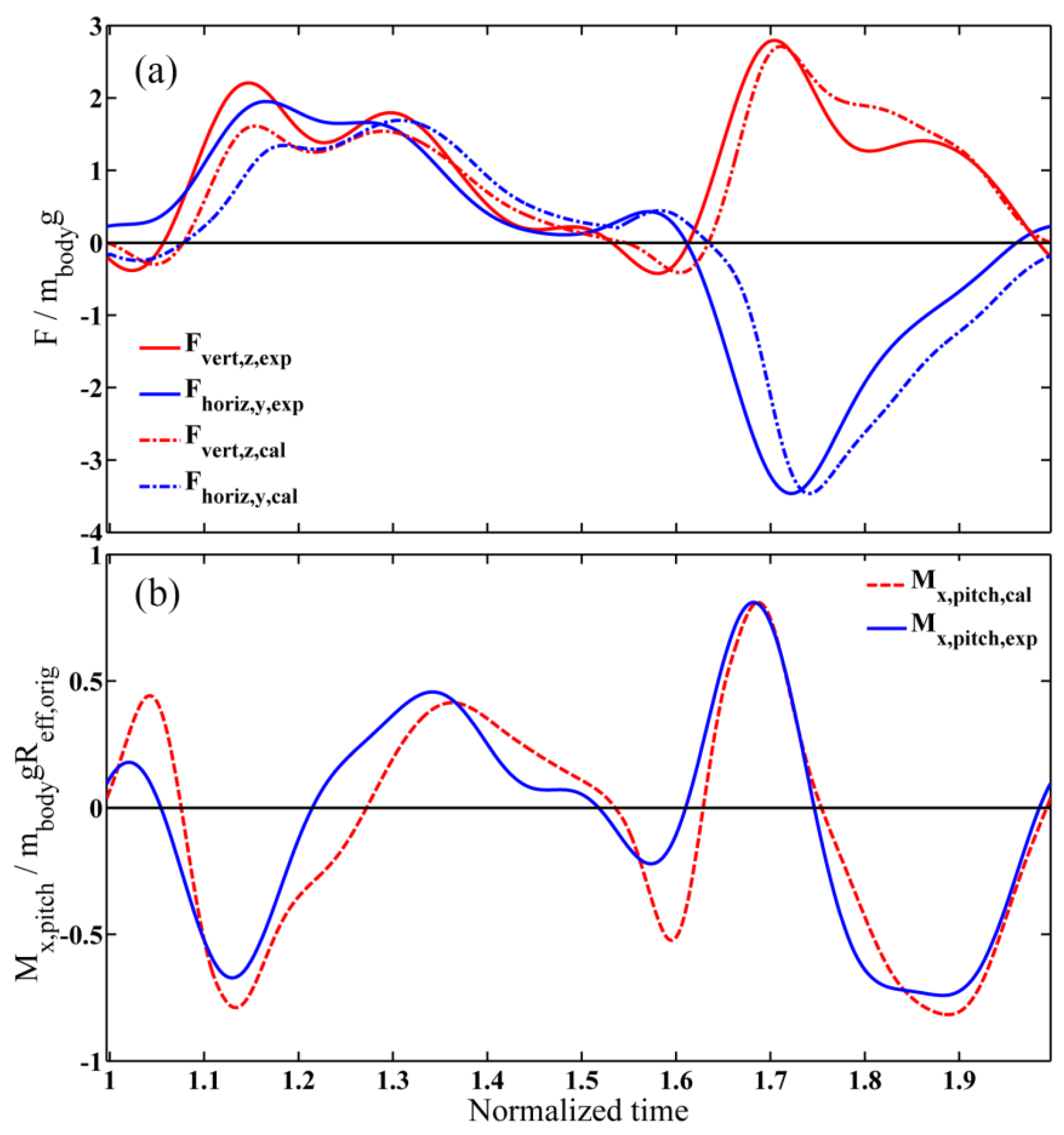
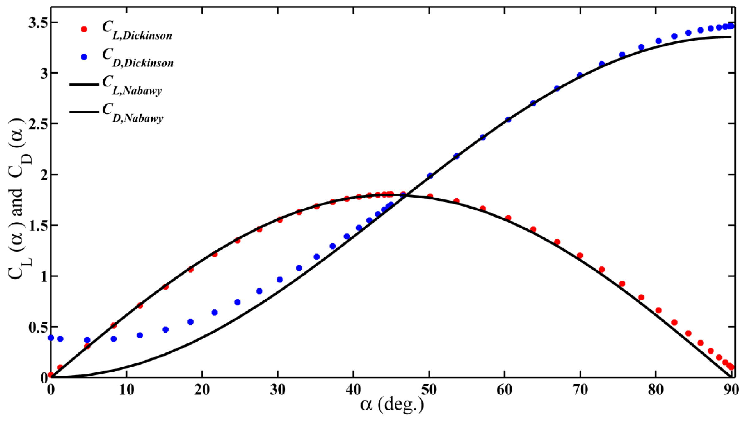
4.5. Verification and Validation

Frankly speaking, the extended quasi-steady aerodynamic model evolved from the work of Sane et al. [32,35,54] and Whitney and Wood [25] has, in some extent, been verified by their works, where the complete experiments were made by them to confirm its applicability. However, part of the viscous dissipative damping arisen from the velocity gradient of differential rotation for chordwise infinitesimal elements was ignored by them. In spite of this, before the development of the optimization problem, the compatibility of current extended quasi-steady aerodynamic model with experimentally measured results of dynamically scaled robotic fruit fly wing, which replayed the steady hovering wingbeat kinematics [27], needs to be validated.

In order to preferably make a comparison with experimental results, the morphological parameters of wing planform (Table S1), and actual leading-edge profiles (z_le(r)) and trailing-edge profiles (z_tr(r)) for right wing of fruit fly (Table S2) are used to calculate non-dimensional aerodynamic forces and moments parameters. The wing motion inputs are given by steady hovering wingbeat kinematics formulas with Fourier form extracted from the Supplementary Materials [27], without involving deviation angle. Here, for comparison with the experimental results, the vertical and horizontal forces (${}^{rr}F_{\mathrm{horizontal},y}$ and ${}^{rr}F_{\mathrm{vertical},z}$ from (37) and pitch torque (${}^{rr}M_{\mathrm{pitch},x}$, which is equal to ${}^{rr}M_x$ from (40) for two wing planforms in the inertial frame are adopted. The comparisons for yaw and roll torque are neglected. Because they are from the contribution of each wing with an opposite sense of direction, both of their eventual summations are equal to zero at each point during the whole stroke period for bilaterally symmetric wing motions [54].

As shown in Figure 6, the magnitude and trends of calculated instantaneous force and pitch torque have a good agreement with the experimental results [27]. However, see Figure 6a,b carefully, the peak value of calculated vertical force and horizontal force is a little lower than the measured ones, while the peak value of calculated pitch moment is a little higher than the measured one, which might result from the absence of deviation angle, after all the experimental measure replays three DOF wing motions [27,52,53]. What is more, some unsteady aerodynamic mechanism mentioned above might also confirm the inability of the current extended quasi-steady aerodynamic model. The experiments that can explicitly determine the coefficients for rotational aerodynamic force and added-mass force, and chordwise location of COP for various kinds of aerodynamic moments need to be done to better estimate these exceptions.

5. Optimization Problem’s Modeling and Formulation

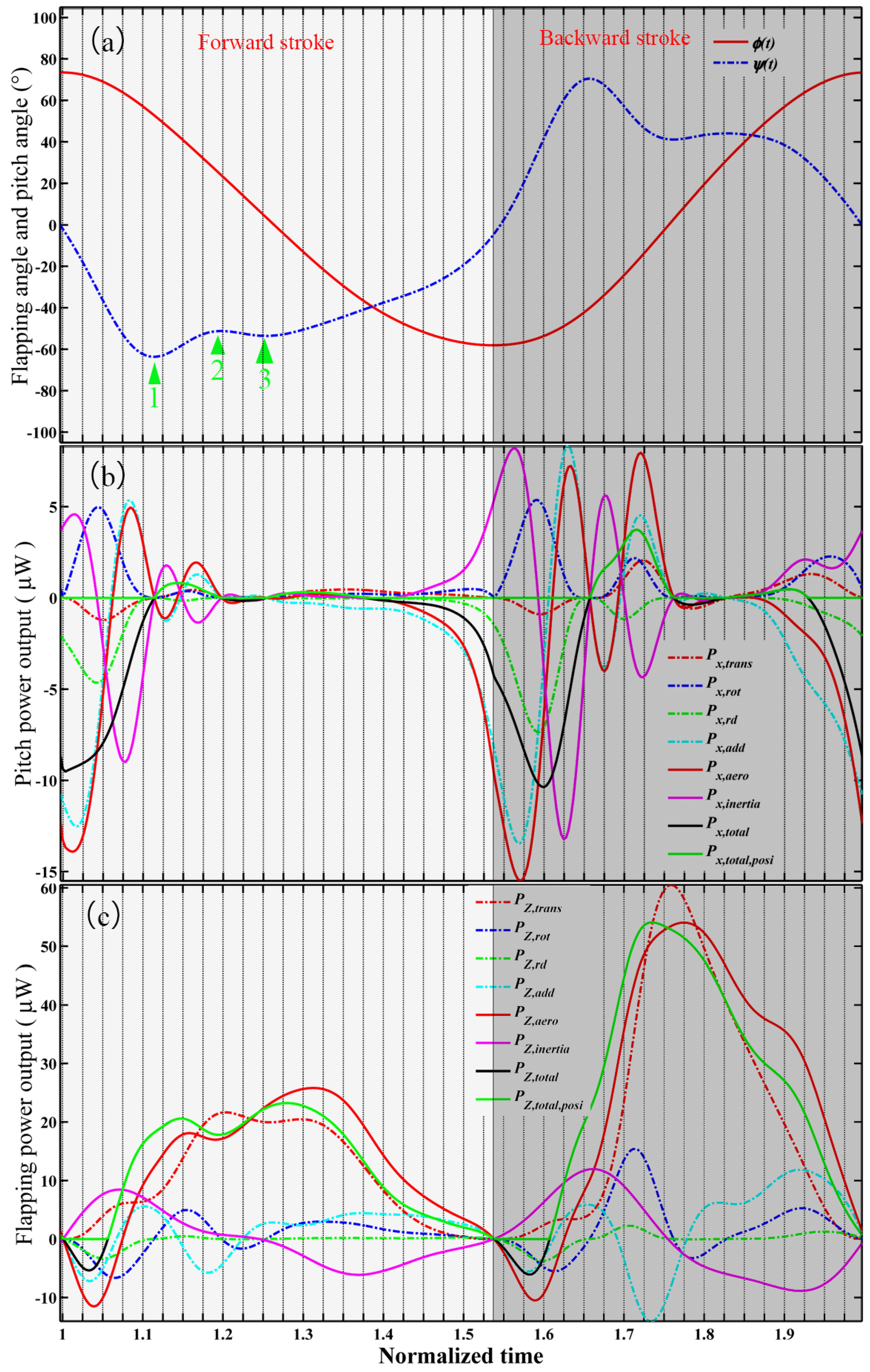
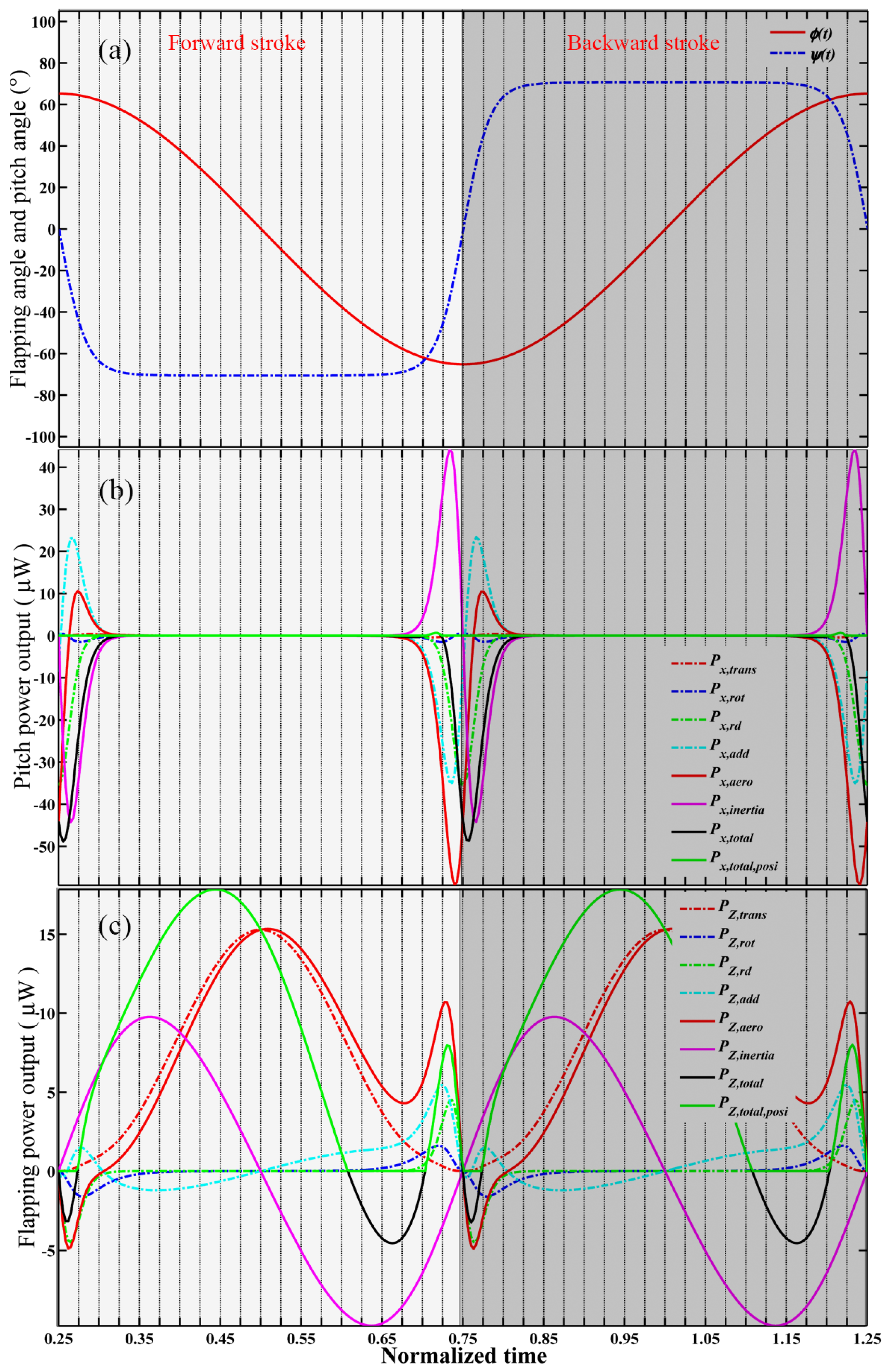
5.1. Power Density Model

Before the development of optimization analysis, three assumptions are made for the power density model [8]. Firstly, the energetic cost consumed by hovering insect only considers the time-averaged positive mechanical power output used to overcome aerodynamic damping and inertial power [54,55,56]. Secondly, the elastic storage can be recovered completely and thus be treated as a part of the negative power of the system [55,56,57]. Thirdly, the wing motions are powered by actuators located at the wing shoulder. Based on these assumptions and Euler equations of a rigid body, the power output from two DOF wing motions about angle i can be written as

$$P_i\left(t\right)=\Xi \left\{{\mathsf{\Omega }}_i\left[I_i{\dot{\mathsf{\Omega }}}_i-M_i^{\mathrm{aero}}\right]\right\},$$

(41)

where [i, j] is a sequence of [ϕ, ψ], I_i and Ω_i are moment of inertia and angular velocity when rotating in angle of i, respectively. The moments of inertia of dynamically scaled wing planform have been expressed in Section 2.3. $\Xi \{·\}$ is a predefined function with the value of 1 for positive internal variable and with the value of 0 for non-positive ones, which is adopted to harness the assumption for completely positive power consumption by taking no account of negative power stored in the system and recovered in the later stroke. $M_i^{\mathrm{aero}}$, which is the component of aerodynamic moment in $\widehat{\varphi }$- or $\widehat{\psi }$-directions, is defined as

$$M_i^{\mathrm{aero}}=\{\begin{array}{cc}{}^{3}M_{\mathrm{total},x}^{\mathrm{pitch}}& i=\psi \\ {}^{1}M_z^{\mathrm{stroke}}& i=\varphi \end{array}.$$

(42)

The inertial power is also included in the later optimization problem [58]. Similarly, take the consistency with much of reported literatures and convenience of measuring optimization objective into consideration [8,34,54,56], we present specific total power P*, i.e., power normalized to mass of insect body:

$$P^{*}=\frac{\Xi \left({\overline{P}}_{\varphi }+{\overline{P}}_{\psi }\right)}{M_{\mathrm{insect}}},$$

(43)

where ${\overline{P}}_{\varphi }$ and ${\overline{P}}_{\psi }$ separately include the aerodynamic power and inertial power (their derivation are detailed in Appendix A, Appendix B and Appendix C, respectively). Here, M_insect is not limited to the body mass of the fruit fly (Table S1), and some other mass arguments can be chosen for the particular design of hovering FWMAV with demand of minimum energy consumption.

5.2. Formulation of the Optimization Problem

The optimization problem is to search for optimal WGP and WKP to minimize the specific power output of hovering insect (LtoW ≥ 1) under different given conditions, such as prescribing wing kinematic pattern and fixed WGP (

Table 3. Original WGP and WKP of hovering fruit fly and optimal WGP and WKP.

Variables	Original WGP and WKP	Optimal WGP with 2D (Left) and 3D (Right) CF,trans (α) b		Optimal WKP	Combined Optimal WGP and WKP with 2D (Left) and 3D (Right) CF,trans (α) b
$R_{\mathrm{eff},\mathrm{vari}}$ (mm)	3.004 a	2.4370	2.6843	3.004 a	3.9813	4.000
$C_{\mathrm{aver},\mathrm{vari}}$ (mm)	0.8854 a	0.9626	0.9882	0.8854 a	1.9600	1.9111
$x_{\mathrm{r},\mathrm{vari}}$ (mm)	0.3289 a	0.3574	0.2315	0.3289 a	1.7845	1.8118
${\widehat{x}}_{0,\mathrm{vari}}$	0.36 a	0	0.1443	0.36 a	0.0001	0.0020
f (Hz)	188.7 a	188.7 a	188.7 a	189.1094	46.6104	60.7851
ϕm	1.1488 a	1.1488 a	1.1488 a	1.1386	1.3076	1.3022
$K_{\varphi }$	null	null	null	0.3733	0.1891	0.1170
ψm (rad)	1.0157 a	1.0157 a	1.0157 a	1.2324	1.2715	1.2287
$C_{\psi }$	null	null	null	4.8336	2.5103	2.5887
ζ (rad)	null	null	null	−1.5708	-1.5169	−1.5391

^a is original data from fruit fly [27]; ^b C_F,trans (α) are 2D or 3D translational aerodynamic coefficients, respectively.

) and constraining AR and Re as follows. Here, AR is introduced as a linear constraint because of its role in mediating stability of LEV. According to the result of statistic analysis over 300 insects, AR of single wing termed Rossby number has an average value near to 3 [59,60]. Here, taking the extension of optimal analysis and feasibility of design in engineering into consideration, we limit the range of AR as

$$2.9\le AR=\frac{R_{\mathrm{eff},\mathrm{vari}}+x_{\mathrm{r},\mathrm{vari}}}{C_{\mathrm{aver},\mathrm{vari}}}\le 4.$$

(44)

The lower bound of AR is an average value for fruit flies [60], and the upper bound refers to the average value of 65 hummingbirds [61]. Moreover, Re as a nonlinear constraint is also introduced to consider the scope of application of quasi-steady aerodynamic model, which has been probed by some researchers [36,62]. Here, by referring to the review of Sun [37], the range of Re is limited as

$$100\le Re=\frac{4{\varphi }_{m}f{R}_{\mathrm{eff},\mathrm{vari}}{C}_{\mathrm{aver},\mathrm{vari}}}{\nu }\le 3000.$$

(45)

So, the optimization problem, which subjects to some tricky nonlinear constraints of Re and LtoW ≥ 1, can be written as:

$$\{\begin{array}{ll}\mathrm{find}& \mathit{x}\\ \min & f\left(\mathit{x}\right)=P^{*}\left(\mathit{x}\right)\\ s.t.& LtoW\left(\mathit{x}\right)=1\\ & {\mathit{x}}_{\min }\le \mathit{x}\le {\mathit{x}}_{\max }\\ & R_{\mathrm{eff},\mathrm{vari}}-4*C_{\mathrm{aver},\mathrm{vari}}\le 0\\ & -R_{\mathrm{eff},\mathrm{vari}}+2.9*C_{\mathrm{aver},\mathrm{vari}}\le 0\\ & 100\nu -4{\varphi }_{m}f{R}_{\mathrm{eff},\mathrm{vari}}{C}_{\mathrm{aver},\mathrm{vari}}\le 0\\ & -3000\nu +4{\varphi }_{m}f{R}_{\mathrm{eff},\mathrm{vari}}{C}_{\mathrm{aver},\mathrm{vari}}\le 0\end{array},$$

(46)

where x is design variables with bound of x_min and x_max, and f(x) is objective function for average positive power density output (P*(x)). AR is the linear equality constraint, and ratio of lift-to-weight (LtoW) and Re are nonlinear inequality constraints. In order to conveniently realize optimization, we convert the constrained optimization into a single objective function with some penalty functions formed by boundary constraints, linear constraints and nonlinear constraints [8]. The single objective function is termed fitness, F(x), which subject to optimized parameter space (ϓ) corresponding to the optimization problem,

$$\min F\left(\mathbf{x}\right)=P^{*}\left(\mathbf{x}\right)+r\Theta \left(1-LtoW\left(\mathbf{x}\right)\right)+s{\displaystyle \sum _{j\in \Upsilon }\frac{\left|{\zeta }_j\right|}{Ma{x}_j-Mi{n}_j}}+\lambda \Theta \left(\left\{Con\right\}\right),$$

(47)

here the nonlinear equality constraint (LtoW ≥ 1) is penalized to be infinitesimally approximate to equality constraint (LtoW ≡ 1) with relative toleration of 10⁻⁸ [8]. $\Theta \left(x\right)$ is set as the Heaviside step function about lift-to-weight’s equality constraint (LtoW = 1) with a positive real penalty factor of r ahead. ζ_j is the distance corresponding to the parameter j outside the range specified by its upper and lower bounds (Max_j and Min_j given in Table 1). Thus, the third item of (47) forms the penalty function about the boundary constraint with a positive real penalty factor of s ahead. Here, $\Theta \left(\left\{Con\right\}\right)$ is also a Heaviside function expression about AR and Re with a positive real penalty factor λ ahead. For the following linear constraint of AR and nonlinear constraint of Re, and $\Theta \left(\left\{Con\right\}\right)$ is constructed by

$$\Theta \left(\left\{Con\right\}\right)=\{\begin{array}{ll}1,\hfill & \mathrm{if}\left(l{c}_1>0\mathrm{or}l{c}_2>0\mathrm{or}nl{c}_3>0\mathrm{or}nl{c}_4>0\right)\\ 0,\hfill & \mathrm{else}\left(l{c}_1\le 0\mathrm{and}l{c}_2\le 0\mathrm{and}nl{c}_3\le 0\mathrm{and}nl{c}_4\le 0\right)\end{array},$$

(48)

where the linear and nonlinear constraints expressions are organized as

$$\{\begin{array}{l}l{c}_1=R_{\mathrm{eff},\mathrm{vari}}-4*C_{\mathrm{aver},\mathrm{vari}}\hfill \\ l{c}_2=-R_{\mathrm{eff},\mathrm{vari}}+2.9*C_{\mathrm{aver},\mathrm{vari}}\hfill \\ nl{c}_3=100\nu -4{\varphi }_{\mathrm{m}}f{R}_{\mathrm{eff},\mathrm{vari}}{C}_{\mathrm{aver},\mathrm{vari}}\hfill \\ nl{c}_4=-3000\nu +4{\varphi }_{\mathrm{m}}f{R}_{\mathrm{eff},\mathrm{vari}}{C}_{\mathrm{aver},\mathrm{vari}}\hfill \end{array},$$

(49)

these expressions are constructed by considering the range of AR and Re, which is necessary for successfully realizing the combined optimization of WGP and WKP.

Here, a hybrid scheme of Genetic Algorithm (GA) and Nelder–Mead simplex algorithm from MATLAB R2011b [63] is adopted to minimize the objective function (F). Firstly, GA for 350 generations with numbers of individuals corresponding to optimized parameters and population size of 100 at each generation is used to approach the global minimal basin. After evolving the population sufficiently to stop according to the stall limit set of generations, then the final best parameter set from GA is taken as initial point for solver of simplex search algorithm, which can efficiently search for the local optimum of the global minimal basin by relaxing each of the parameter sets obtained by GA. In the iterations of the simplex search algorithm, relative tolerances of 10⁻⁸ for fitness function and all constraint parameters are set as stall limits of convergence for the final solution by considering computation cost. Here, all of the values of r, s and λ are chosen to be 2000 [8].

6. Optimization Results and Analysis

6.1. WGP Optimization Results

Firstly, the sole optimization of WGP with 3D translational aerodynamic coefficients is executed to minimize the hovering specific power output. Here, the WKP are unchanged and completely equal to the data from approximately steady hovering fruit fly (Table 3, as illustrated in Figure 7a). The optimal results are listed in Table 3 and

Table 4. The estimated values of hovering fruit fly and optimization results.

	For Original WGP and WKP	For Optimal WGP with 2D (Left) and 3D (Right) CF,trans (α)		For Optimal of WKP	For Combined Optimal WGP and WKP with 2D (Left) and 3D (Right) CF,trans (α)
AR	3.7643 a	2.9029	2.9506	3.7643 a	2.9417	3.0411
Re	172.8926 a	157.6046	168.8122	171.7340	186.1461	237.6147
LtoW-1	0.2890	3.7 × 10−8	5.2 × 10−8	1.6 × 10−8	3.0 × 10−8	1.9 × 10−8
${\langle {}^{1}F_{\mathrm{vert},\mathrm{z}}\rangle /\langle {}^{1}F_{\mathrm{horiz},\mathrm{x}}\rangle }_{\mathrm{rms}}$	0.8834	0.8855	0.8960	1.1241	1.1089	1.0173
$\langle P^{\mathrm{aero}}\rangle /\langle P^{\mathrm{inertial}}\rangle$	8.4327	5.8237	5.7343	1.4711	3.7811	2.4905
P* (Wkg−1)	33.0097 b	20.4839 b	21.1160 b	9.1074	4.7867	6.7156

^a Here, AR and Re are obtained by known WGP and WKP of hovering fruit fly; ^b The value of P* is approximate to the reported one [8,30,68].

. Then the pitch power output and flapping power output of a single wing planform separately along the pitch axis of wing planform and flapping axis of the right wing root frame are estimated again in terms of (41) with the optimal WGP and known WKP (as illustrated in Figure 7b,c). Both the pitch power output and flapping power output include aerodynamic power and inertial power, respectively. The aerodynamic power consists of four components, which are from translational circulation effect, rotational circulation effect, rotational damping, and added-mass effect. In addition, the positive mechanical pitch and flapping power output utilized to estimate time-averaged power density in optimization model (41) and (43) are also shown (Figure 7b,c). Here, it is not difficult find that pitch power consumption mainly distributes around the pitch reversal while flapping power consumption distributes during the large range of the midstroke and peaks near to the midstroke.

For pitch aerodynamic power (P_x,total) during the forward stroke (Figure 7b), the added-mass power (P_x,add) dominates other three terms, the subdominant term belongs to rotational circulation power (P_x,rot), and the third one is rotational damping power (P_x,rd), while the translational circulation power (P_x,trans) has the minimum contribution to pitch power consumption. Their synergistic effect spans a rapidly varying pitch interval composed of three pitch reversal segments, and two positive peaks of pitch aerodynamic power distribute at previous instant of the first and second pitch reversal points, where the pitch velocity or slope of wing pitch angle is maximum (Figure 7a,b). The pitch inertial power (P_x,inert) is reverse to the pitch aerodynamic power; their mutual subtraction results in a positive peak of total pitch mechanical power output (P_x,total,posi) around the middle of the first and the second pitch reversal points. For the backward stoke, a similar trend of pitch power distribution can be observed, although with some differences in amplitude. Namely, the amplitudes are larger than those for forward stroke. This is due to a faster stroke being completed in the backward stroke (Figure 7a,b).

For flapping aerodynamic power (P_Z,total) during the forward stroke (Figure 7c), the translational circulation power (P_Z,trans) dominates the other three terms, the subdominant term belongs to added-mass power (P_Z,add), and the third one is rotational circulation power (P_Z,rot), while the rotational damping power (P_Z,rd) has a minimum contribution to flapping power. The flapping inertial power (P_Z,inert) is positive during translation acceleration and negative during translation deceleration. Their synergistic effect results in two positive peaks of total flapping mechanical power output (P_Z,total,posi) occurring around the middle of the forward stroke, which is different from the situation for the backward stroke. In the backward stroke, there is only one positive peak because a faster backward stroke leads to a larger translational aerodynamic power output than inertial power. Eventually, the positive total flapping mechanical power output is nearly consumed during the whole stroke except at the interval of stroke reversal where a minor negative P_Z,add might be stored in elastic joint or dissipated.

It is worth noting that the asymmetries of amplitudes for pitch power output and flapping power output are observed in Figure 7b,c, which must result from the fact that different split time are consumed by the forward stroke and backward stroke for hovering steady wingbeat motion of fruit fly.

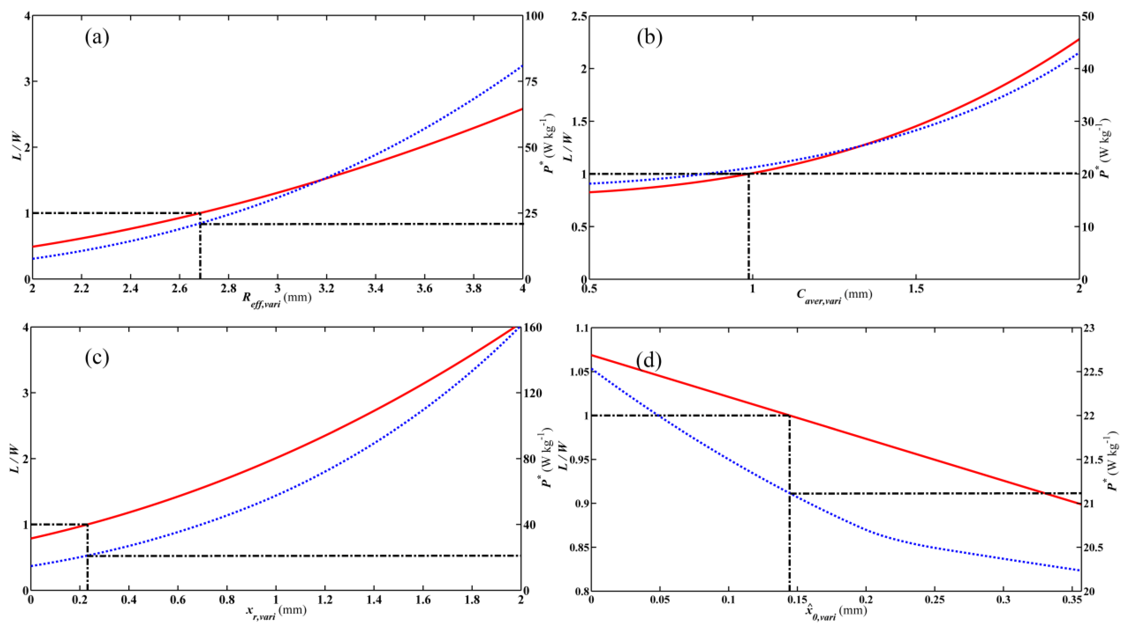
6.2. Sensitivity Analysis for Optimal WGP

Given the optimized WGP listed in Table 3, the effect of a perturbing single parameter on lift-to-weight ratio and power density is analyzed to gain insight of the reason why the optimized WGP can produce power-efficient lift to maintain the insect’s aloft hovering. It is necessary to dissect how the most power-efficient lift-to-weight ratio changes with one parameter of WGP while keeping other parameters unchanged and equal to their optimal values. As shown in Figure 8a–c, the lift-to-weight ratio and power density consistently and monotonically increase with wing length ($R_{\mathrm{eff},\mathrm{vari}}$), average chord ($C_{\mathrm{aver},\mathrm{vari}}$) and wing-root offset ($x_{\mathrm{r},\mathrm{vari}}$), although there is an interplay between WGP via AR except for the parameter for non-dimensional location of pitch axis (${\widehat{x}}_{0,\mathrm{vari}}$). This indicates that the conflict between lift-to-weight ratio and power density is unavoidable because additional lift production must result in an increase of power consumption. Thus, the optimal values for these parameters, which are loosely restricted by approximate nonlinear equality constraint (LtoW ≡ 1), were found by the resulting simplex algorithm. The lift-to-weight ratio and power density consistently and monotonically decrease with ${\widehat{x}}_{0,\mathrm{vari}}$ (Figure 8d), which arises from the fact that lift changes with ${\widehat{x}}_{0,\mathrm{vari}}$ due to variation of rotational circulation coefficient (C_R ) with ${\widehat{x}}_{0,\mathrm{vari}}$ [32,64] although the inertial power shall reduce with the pitch axis shifting to trailing edge. Thus, the optimal value of ${\widehat{x}}_{0,\mathrm{vari}}$ with maximum rotational circulation coefficient is a reasonable value under primary condition of lift balancing weight.

Furthermore, the sole optimization results of WGP for 2D translational aerodynamic coefficients (Table 3) are also used to plot instantaneous power output (as seen in Figure S1 of Supplementary Materials for compactness). The sensitivity analysis of the single parameter is shown in Figure S2. No obvious distinction is observed in the visualization results involving 3D and 2D translational aerodynamic coefficients although there is a small difference in amplitude, which directly indicates that the adopted 3D translational aerodynamic force coefficients have little effect on the eventual optimization results of WGP and indirectly shows that the variation of wing shape only brings little influence on lift and power density by probable way of influencing translational aerodynamic coefficients.

6.3. WKP optimization Results

As for WKP optimization, the sole optimization of WKP is performed to minimize the specific power output of a hovering insect by using 2D translational aerodynamic coefficients, which is also formulated as Equation (47) but does not involve linear equation constraints for AR. For this optimization problem, the WGP are unchanged and they are taken from the actual morphological parameters of fruit fly (as listed in Table S1 and S2). The optimal results are also listed in Table 3 and Table 4. The optimal wing kinematic pattern is characterized by round trapezoidal profile for pitch angle, and harmonic shape profile for flapping angle (Figure 9a). The round trapezoidal pitch angle signifies the pitch reversal of wing must be completed at certain faster time scale regulated by C_ψ. Moreover, the geometry angle of attack needs to be kept constant during the large range of the midstroke. Here, the optimal harmonic shape flapping angle profile is different from those reported by Nabawy and Corwther and Taha et al. [12,42], who acquired the triangular flapping angle profile. This must be attributed to the fact that the effect of rotational circulation mechanism and added-mass effect on lift and power consumption has been neglected in their power consumption estimating model.

Similarly, once acquiring optimal WKP, the pitch power output and flapping power output of a single wing planform can be estimated again with given fixed WGP of fruit fly (Table 3) and illustrated in Figure 9b,c. Likewise, the pitch power consumption mainly distributes around the pitch reversal while flapping power consumption distributes during the large range of the midstroke, and peaks before the middle of the half stroke due to the peak of flapping inertial power before half of the forward stroke.

For pitch aerodynamic power (P_x,total) during the forward stroke (Figure 9b), the added-mass power (P_x,add) has a nearly equivalent peak to the rotational damping power (P_x,rd), which arises from the larger pitch velocity and acceleration induced by faster time scale of pitch angle during pitch reversal. The translational circulation power (P_x,trans) and rotational circulation power (P_x,rot) make minimum contribution to pitch power consumption. Their synergistic effect spans the interval of pitch reversal, and one positive peak of pitch aerodynamic power occurs at the end of the pitch reversal, which is mainly contributed by P_x,add (Figure 9b). The pitch inertial power (P_x,inert) is likewise reverse to the pitch aerodynamic power, their mutual subtraction results in a minor positive peak of total pitch mechanical power output (P_x,total,posi) around the pitch starting point (Figure 9b). For the backward stoke, a completely equivalent trend of pitch power distribution can be observed without any asymmetrical amplitude distribution like the situation in Figure 7b.

For flapping aerodynamic power (P_Z,total) during the forward stroke (Figure 9c), the translational circulation power (P_Z,trans) dominates the other three terms, the subdominant term belongs to added-mass power (P_Z,add), and the third one is rotational damping power (P_Z,rd), while the rotational circulation power (P_Z,rot) has minimum contribution to flapping power consumption. The flapping inertial power (P_Z,inert) is likewise positive during the translation acceleration and negative during the translation deceleration. Their synergistic effect results in two positive peaks of total flapping mechanical power output occurring before the middle of forward stroke and at the middle of accelerating pitch interval, respectively. The former main peak should be attributed to the influence of peak of flapping inertial power before half of forward stroke. The latter subordinate peak is contributed by peak distribution of P_Z,add, P_Z,rd, and P_Z,rot, all of them have peak amplitude around the point locked by the maximum slope of pitch angle. Eventually, the positive total flapping mechanical power output (P_Z,total,posi) is nearly consumed during large part of the whole stroke except at the interval before the starting of pitch reversal and short interval of starting of next half stroke. In these two intervals, the flapping inertial power and added-mass power term are negative and might be stored in elastic joint or dissipated. A completely equivalent trend of flapping power distribution is observed for backward stoke. Here, the pitch power and flapping power output distribution is different from the situation in Figure 7b,c because of the completely different wing kinematic profile adopted.

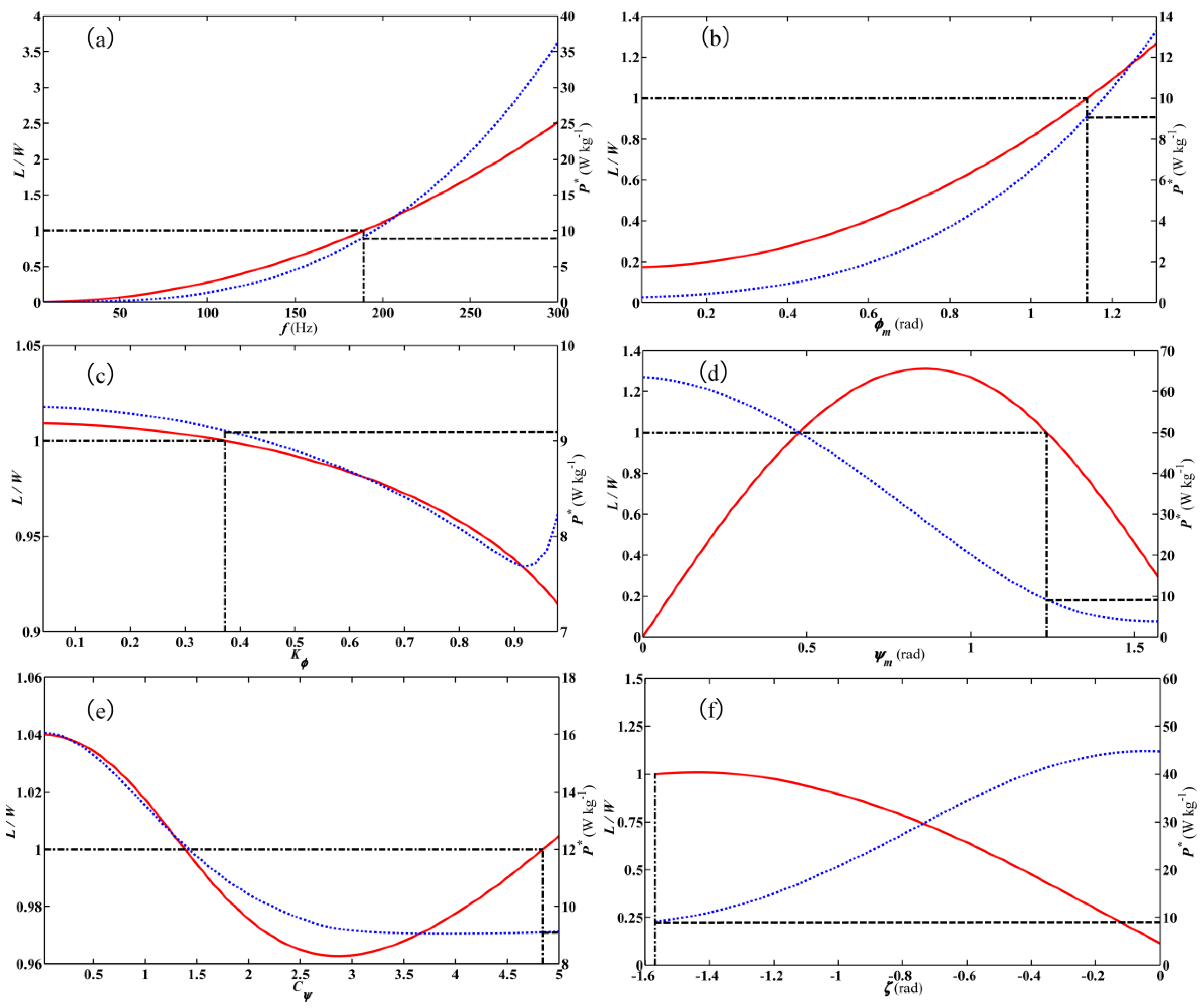
6.4. Sensitivity Analysis for Optimal WKP

Similarly, given optimized WKP listed in Table 3, the effect of perturbing single parameter on lift-to-weight ratio and power density is analyzed while keeping other parameters unchanged (Figure 10). Obviously, there is a sound interplay between some WKP due to the nonlinear constraint of Re formed by frequency, flapping amplitude and part of the fixed WGP.

The lift-to-weight ratio and power density consistently and monotonically increase with flapping frequency and amplitude of flapping angle (ϕ_m) (Figure 10a,b). Similarly, this indicates that the conflict between lift-to-weight ratio and power density also occurs. For the regulating parameter of flapping angle (K_ϕ), both of lift and power decrease monotonically during large part of the interval of variable K_ϕ. The optimal value of K_ϕ determines the profile of the flapping angle approaching the harmonic shape such that the lift constraint is met although the power density does not achieve its minimum value (Figure 10c).

The amplitude of the pitch angle (here, ϕ_m = 70.6 deg, Table 3) corresponds to the mid-stroke value of the angles of attack (α = 19.4 deg), which is an optimal value of aerodynamic efficiency for translational aerodynamic lift and drag coefficients. This proximate value has been reported in sole WKP optimization [8,13]. After this optimal value (Figure 10d), the lift constraint cannot be met although the power density decreases further. The regulating parameter of pitch angle (C_ψ), which strictly controls the variable time scale of pitch reversal, indirectly affects lift and power density through added-mass force, rotational circulation force and damping force during pitch reversal interval. The lift firstly decreases monotonically with C_ψ during the first approximate half of the variable interval and then increases monotonically during the second half of the variable interval (Figure 10e). The power density decreases monotonically with C_ψ until it reaches a constant value (Figure 10e). The optimal value (C_ψ = 4.8, Table 3) approaches the prescribed upper bound of C_ψ (Table 1), which determines the pitch angle featuring the round trapezoidal profile. Lastly, the pitch phase offset relative to the flapping angle (ζ), which affects rotational circulation effect and unsteady wake capture [34], targets an optimal value of −π/2 for current power density optimization model. Any deviation from this value will dissatisfy the lift constraint when other optimal parameters are fixed (Figure 10d).

6.5. Combined Optimization Results for WGP and WKP

Lastly, for the combined optimization of WGP and WKP, the single objection function including nonlinear penalty for lift-to-weight constraint, penalty of boundary constraints, linear penalty of AR constraint, and nonlinear penalty of Re constraint is performed to minimize specific power output by using 3D translational aerodynamic coefficients (refer to Equation (47)). Here, both WGP and WKP are variable and constrained in particular boundary listed in Table 1. As seen from the optimal results listed in Table 3 and Table 4, the pitch angle is also characterized by round trapezoidal profile but with lower flapping frequency and shorter pitch time scale controlled by C_ψ than for those for sole WKP optimization, and the flapping angle also varies with harmonic shape profile (Figure 11a). Here, it is worth noting that the trapezoidal pitch angle profile might not be an optimal solution in engineering. Since this profile is not easy to be realized on account of the actuator mode selection for the wingbeat motion of FWMAV [13]. Thus, the dynamics problem for this kind of pitch motion needs to be probed deeply in theory, and the feasible design for FWMAV with active or passive pitch motion may require a large amount of elaborate redesign and experiments with or without torsional hinge or/and actuator along the pitch axis [2,5,33,65,66].

The pitch angle amplitude determines the geometric angle of attack at the midstroke. Thus, it is always expected for flapping flight that the optimal angle of attack will bring about the most efficient translational lift and drag coefficient to minimize power consumption. In this study, the optimal pitch angle amplitude from the results of sole WKP optimization (ψ_m = 70.6 deg) and combined optimal WGP and WKP (ψ_m = 70.4 or 72.9 deg) is nearly equivalent (Table 3), both of them are approximately equal to the reported value (ψ_m = 72.7 deg for fruit fly) [8].

The pitch phase offset mainly influences rotational circulation force and wake capture [34]. Because the current power density model, which is based on extended quasi-steady aerodynamic model with the absence of some other unsteady lift effect (such as wake capture), is set to achieve the minimization of power consumption but not the maximum of lift, thus the symmetry pattern between flapping angle and pitch angle is dug out when the zero pitch angle crosses to the stroke reversal point. Here, the optimal values of pitch phase offset from the results of sole WKP optimization and combined optimal WGP and WKP is approximate to −π/2 (Table 3), and both of them are similar to the reported value [8]. Moreover, all of the WGPs approach their upper bounds except the non-dimensional location of the pitch axis, which is near to zero. The combined optimal result with the feature of larger WGP and lower frequency arises from the fact that the strong linear and nonlinear coupling relationships between WGP and WKP via AR and Re have an intense effect on the optimization procedure.

Likewise, for the combined optimal WGP and WKP, the pitch power output and flapping power output of a single wing planform are estimated again and illustrated in Figure 11b,c. The time histories of those power outputs have similar trend to those from sole WKP optimization but with different amplitude distribution due to different optimal WGP and WKP adopted (Table 3, Figure 9b,c and Figure 11b,c). For pitch aerodynamic power (P_x,total) during forward or backward stroke (Figure 11b), the added-mass power (P_x,add) dominates the other three terms, the subdominant term belongs to the rotational damping power (P_x,rd), and the third one is rotational circulation power (P_x,rot), while the translational circulation power (P_x,trans) makes minimum contribution to pitch power consumption. The pitch inertial power (P_x,inert) is reverse to P_x,add but with nearly equivalent amplitude, their mutual subtraction leads the positive peak of total pitch mechanical power output (P_x,total,posi) near to zero during the whole stroke (Figure 11b), which is not observed in the results from sole WGP or WKP optimization. Moreover, the main time interval of pitch reversal occupied by pitch power consumption is wider than that for sole WKP optimization, which results from the fact that the pitch regulating parameter of C_ψ is smaller than the latter one, thus the pitch reversal completes slowly. For flapping aerodynamic power (P_Z,total) during the forward or backward stroke (Figure 11c), the translational circulation power (P_Z,trans) dominates the other three terms, the subdominant term belongs to added-mass power (P_Z,add), and the third one is rotational circulation power (P_Z,rot), while the rotational damping power (P_Z,rd) has minimum contribution to flapping power consumption. All of them may be synergistically generated from lower frequency, larger flapping amplitude, shorter pitch time scale (C_ψ) and larger WGP except non-dimensional location of the pitch axis in comparison to the situation of sole WKP optimization (Table 3, Figure 9a and Figure 11a). The flapping inertial power (P_Z,inert) is likewise positive during the translation acceleration and negative during the translation deceleration but with relatively lower amplitude than that for sole WKP optimization. Their synergistic effect results in two positive peaks of total flapping mechanical power output occurring before the middle of half stroke and at the middle of the accelerating pitch interval, respectively. The reason why these positive peaks occurred at these locations is very similar to that analyzed for sole WKP optimization. The positive value of the total flapping mechanical power output (P_Z,total,posi) nearly spans the whole stroke except at the short interval of starting of next half stroke where P_Z,rot and P_Z,rd are negative and might be stored in elastic joint or dissipated.

6.6. Sensitivity Analysis for Combined Optimal WGP and WKP

Similarly, given the combined optimal WGP and WKP listed in Table 3, the effect of perturbing single parameter on lift-to-weight ratio and power density is also analyzed. As seen in Figure 12, the distribution feature of some of optimal values in their own constraint boundary is completely similar to those for sole WGP or WKP optimization although with different peak or amplitude difference of power density, such as the effective variable wing length ($R_{\mathrm{eff},\mathrm{vari}}$), variable average chord ($C_{\mathrm{aver},\mathrm{vari}}$), wing-root offset ($x_{\mathrm{r},\mathrm{vari}}$), and non-dimensional location of pitch axis (${\widehat{x}}_{0,\mathrm{vari}}$) for WGP (Figure 8 and Figure 12a–d), and flapping frequency, amplitude of flapping angle (ϕ_m), amplitude of pitch angle (ψ_m) and pitch phase offset (ζ) for WKP (Figure 10a,b,d,f and Figure 12e,f,h,j). Here, the optimal values for non-dimensional location of the pitch axis, which consistently approach the leading edge for the optimization involving WGP (Table 3), is only the numerical solution but not reflect the real situation since the pitch axis might be not a straight line. In engineering design, the location of pitch axis needs to be determined by experimentally measuring the optimal angle of attack [57]. In order to survive in a complex environment such as predation or evading maneuverability with limited energy, fruit fly might evolve to have pony-size WGP adaptive to its body size in millimeter scale but high flapping frequency and large flapping amplitude under the strategy of minimum power consumption. For the design of FWMAV, high frequency will lead to the dilemma of designing actuator and avionics system. Thus, the optimal large-sized wing length and average chord might be favorable to lower flapping frequency with minimum power consumption.

Moreover, the flapping frequency and flapping amplitude are two competitive parameters to realize the production of high lift and minimum power consumption. The flapping amplitude determines the travel distance of chordwise section of wing planform, and thus the vortex dynamical evolutionary process. While high flapping frequency means high frequency evolution of highly unsteady flow field, namely, the starting vortex, LEV, trailing edge vortex, wing tip vortex, downwash vortex and wake vortex are interwoven and interact at different instants thus influence the aerodynamic performance of wing planform [62,67]. As mentioned above, lower flapping frequency and appropriate flapping amplitude is expected for the designer to successfully solve the engineering problem of Bio-FWMAV although simultaneously compromising high maneuverability yielded by high lift from unsteady mechanism.

The distinction of sensitivity trend for optimal regulating parameter of flapping angle (K_ϕ) and pitch angle (C_ψ) can be observed between Figure 12g,i and Figure 10c,e for sole WKP optimization. In Figure 12g, the lift decreases monotonically with K_ϕ during the whole variable interval, but the power density nearly maintains constant during the approximate front half of variable interval, and then monotonically increases during the second half of variable interval. The sensitivity trend of power density about K_ϕ is different from the situation shown in Figure 10c, which might arise from the effect of the strong coupling relationship between WGP and WKP via AR and Re when acquiring the sensitivity data of power density about K_ϕ with other optimal WGP and WKP unchanged. However, the flapping angle still manifests harmonic shape profile with an optimal value (K_ϕ = 0.189, Table 3) such that the lift constraint is met while the power density achieves the minimum. In Figure 12i, the lift decreases slowly during approximate front half of variable interval, then increases monotonically with C_ψ during the second half of variable interval, while the power density nearly monotonically decreases with C_ψ. The sensitivity trend of lift and power density about C_ψ is also different from the situation shown in Figure 10e, which might likewise arise from the effect of strong coupling relationship between WGP and WKP. When the lift constraint is met, the optimal value C_ψ is equal to 2.51 (Table 3), which also determines round trapezoidal pitch angle profile with slower time scale during the pitch reversal than the one for sole WKP optimization.

Likewise, the combined optimal WGP and WKP for the 2D translational aerodynamic coefficients (Table 3 and Table 4) are also used to plot the instantaneous power output (as seen in Figure S3 of Supplementary Materials). The sensitivity analysis of a single parameter is shown in Figure S4. The qualitative similarity of the visualization results involving 3D and 2D translational aerodynamic coefficients is also observed although with little difference of amplitude.

7. Discussion

Due to the synergistic influence of WGP and WKP on the aerodynamic performance of wing planform of hovering insect and thus eventual power consumption in linear or nonlinear coupled way by AR and Re, any parameter set obtained by sole WGP or WKP optimization is not the global optimal one in global design variable space. This has been verified by the results listed in Table 4.

The values listed in Table 4 are acquired by substituting the original WGP and WKP of hovering fruit fly and optimized parameters from five cases of optimization into the power density model without embedding hybrid-GA. It is interesting to find that the linear constraints (AR) and nonlinear constraints (Re) for five cases of optimization do not manifest substantial variation. The power density obtained by combined optimal WGP and WKP is lower than that from sole WGP or WKP optimization, which may be due to the influence of strong coupling constraint of AR and Re on global optimal parameters. Moreover, the value of power density obtained by solely optimal WKP is less than the one reported by Berman and Wang [8], which might be due to two factors. The first one is that the stroke plane deviation angle has been ignored here. The second factor must be the crucial one to improve the estimation of power density. That is a much more reasonable assumption about non-dimensional chordwise distribution of COP for translational and rotational circulation force introduced into current extended quasi-steady aerodynamic model to estimate the rotational circulation power consumption. This assumption is different from the one made by Berman and Wang. In their work, they also assume that the translational and rotational circulation forces have a similar chordwise distribution of COP, but the chordwise location was assumed to be fixed at the middle point of each strip element. This does not conform to the empirical formula fitted from experimentally measured data [47,48]. Thus, their result about the power density might be over-estimated except including the power consumption from stroke plane deviation motion. All of the power density values for optimzation of WGP or/and WKP are much lower than the estimating value of approximate steady hovering flight of fruit fly (Table 4). It is worth noting that the difference value between the ratio of lift-to-weight and one (LtoW-1) is limited by relative toleration of 10⁻⁸ (Table 4), which is larger than the one used by Berman and Wang [8]. We choose this larger relative toleration just by considering the calculation cost. Frankly speaking, the lower this difference value is prescribed, the better the condition of nonlinear equality constraint is satisfied.

Moreover, the ratio of vertical force and horizontal force for combined optimal WGP and WKP is approximate to the one for sole WKP optimization and larger than the one for sole WGP optimization. This should be attributed to the optimal WKP producing an efficiency wing motion pattern, which is characterized by the relatively lower geometric angle of attack. Since much more appropriate translational lift coefficient and lower drag coefficient will be yielded at lower geometric angle of attack in comparison with the situation of larger geometric angle of attack.

The ratio between aerodynamic power including added-mass component and inertial power derived from moments of inertia of wing planform for sole WGP optimization is lower than the original one. This arises from an increase of inertial power induced by the shift of variable non-dimensional location of pitch axis (${\widehat{x}}_{0,\mathrm{vari}}$) towards the leading edge, which possesses relatively shorter wing length and wider average chord length in comparison to the original ones (Figure 13, Table 3 and Table 4). In Figure 13, the original fruit fly wing planform outline is plotted with a black crude solid line, the dynamically scaled wing planforms for optimal WGP optimized with 2D or 3D translational aerodynamic coefficients (illustrated by blue and green crude solid line, respectively, ‘wo’ denotes WGP optimization) and for combined optimal WGP and WKP optimized by the 2D or 3D translational aerodynamic coefficients (illustrated by red and cyan crude solid line, respectively, ‘co’ denotes combined optimization) are also illustrated for comparison. The frame of X_sO_sZ_s, wing roots, COM and variable pitch axis for two wing planforms are also included. As seen in Figure 13, for dynamically scaled wing with non-dimensional conformal feature of fruit fly wing, there is a relatively diminutive difference between the optimized 2D wing outline and 3D wing outline. Likewise, this little difference directly indicates that the adopted 3D translational aerodynamic force coefficients have little effect on the eventual optimization results of WGP (Table 4). And it in turn indirectly shows that the variation of wing shape only brings little influence on lift and power density by probable way of influencing translational aerodynamic coefficients. After all, the LEV for translational circulation aerodynamic force may be maintained and attached even on dynamical scaled insect wings with lower Re and AR (Table 4) due to the attenuating effect of the downwash induced by the tip vortex and wake vorticity.

Moreover, the ratio of aerodynamic power and inertial power for combined optimal WGP and WKP is lower than the one for original and optimal WGP, which should result from an increase of inertial power with larger WGP except the value of ${\widehat{x}}_{0,\mathrm{vari}}$. Moreover, lower flapping frequency and faster pitch reversal regulated by C_ψ also induced higher inertial power (Figure 13, Table 3 and Table 4). While the ratio of aerodynamic power and inertial power for solely optimal WKP is much lower than that for combined optimal WGP and WKP in spite of WGP fixed during the optimization of WKP. This could be mainly attributed to a larger pitch regulating parameter (C_ψ) inducing much higher inertial power (Table 3 and Table 4).

8. Conclusions

In this paper, the separate or combined optimizations of wing geometry parameters or/and wing kinematic parameters are systematically performed to minimize the energy of flapping wing hovering flight, firstly on the basis of extended quasi-steady aerodynamic model by using hybrid-GA. Before the elaboration of the optimization problem, the parametrization description of dynamically scaled wing with non-dimensional conformal feature of insect-scale rigid wing is firstly proposed. This parametrization method provides an effective simplifying method for aerodynamic analysis based on insect-scale rigid wings’ non-dimensional outline, and thus the feasibility for optimization involving WGP. Then, the extended quasi-steady aerodynamic model is derived on basis of previous quasi-steady aerodynamic model by using 2D or/and 3D translational lift and drag coefficients with consideration of the possible effect of any variation of wing shape on the aerodynamic coefficients. Further, the objective function of optimization is formed by hovering flight power density with additional penalty items for lift-to-weight ratio, boundary constraints, linear constraint of AR and nonlinear constraint of Re.

For five cases of separate or combined optimization for WGP or/and WKP, given unchanged wing kinematics pattern or WGP or no arguments input, we performed the optimizations of WGP or/and WKP to minimize the energy of flapping wing hovering flight by using hybrid-GA formed by the GA and Nelder–Mead simplex algorithm. The optimization results show that the combined optimization of wing geometry and kinematic parameters can obtain lower flapping frequency, larger wing geometry parameters and lower power density in comparison with those from other cases of optimization. The amplitude of flapping angle for the optimization involving WKP is close to their prescribed upper bound. All of these results arise from the effect of strong coupling relationship between WGP and WKP via AR and Re when the minimum power density is obtained under the constraint of lift balancing weight. Moreover, the flapping angle for the solely optimal WKP and combined optimal WGP and WKP manifests harmonic shape profile, and the pitch angle possesses round trapezoidal profile with certain faster time scale of pitch reversal controlled by its regulating parameter. The dynamics problem for flapping motion with or without resonant frequency to the drivetrain and pitch motion with constant angle of attack around midstroke needs to be studied deeply in theory, and in the bio-design of FWMAV with active or passive pitch motion through including or excluding the torsional hinge or/and actuator along pitch axis. In addition, no obvious distinction is observed in the optimal visualization results involving WGP for the case of 3D and 2D translational aerodynamic coefficients although there is little difference in amplitude, which directly indicates that the adopted 3D translational aerodynamic force coefficients have little effect on eventual optimization results involving WGP and indirectly shows that the variation of wing shape only brings little influence on lift and power density by probable way of influencing translational aerodynamic coefficients.

The advantage of currently proposed combined optimization framework is obvious: it can drastically reduce the computational cost for current complicated optimization problem and quickly provide the fundamental optimized parameters of biomimetic flapping wing micro aerial vehicle at the stage of conceptual design. However, there are two limitations worthy of being noted. Firstly, the extended quasi-steady aerodynamic model presented is unable to take some feeble unsteady effect mentioned above into consideration, thus a much higher fidelity model or efficiency numerical method, such as CFD, need to be set up to perform the combined optimization with higher computation accuracy. Secondly, the parametrization description of dynamically scaled wing with non-dimensional conformal feature of smaller insect-scale wing is based on the assumption of rigid wing, which is characterized by smaller wing effective length and average chord length, thus lower inertial mass property relative to the larger wing planform, such as the hawkmoth wing. Thus, the aeroelastic coupling effect of wing planform under the external acting force from the aerodynamic force and inertial force of wing planform itself cannot be considered. After all, every kind of material will have a slight deformation even at a lower external applied load. So once the designers are in pursuit of combined optimization results with much higher fidelity and accuracy, the aeroelastic problem needs to be solved during the aerodynamic model. It is well known that the larger the feature size of wing planform is, the larger the inertial force the wing planform itself will be applied, so the larger wing planform is more apt to deform. However, in current research for dynamical scaled fruit fly wing planform with smaller feature size and lower inertial mass property, its upper boundary of spanwise length shall not exceed four millimeters, thus, the assumption of rigid wing planform is feasible for the little scale rigid wing planform, which has been confirmed by much previous literatures. In short, the currently proposed combined optimization framework on the basis of extended quasi-steady aerodynamic model is more applicable to the situation of predication and optimization of aerodynamic performance and efficiency of bio-insect scaled flapping wing micro aerial vehicles assembled with rigid wing planform, which possesses smaller feature size.

From the aspects of theory and experiment, ensuing studies for bio-design of FWMAV should focus on the optimization involving wing morphology with different outlines of leading edge and trailing edge bio-inspired by other insect wings or artificial wings with regular shape and broader wing kinematics pattern. What is more, the problem of energy minimum pertinent to forward flight and other maneuvering flight need to be probed, although a much more complicated power model will emerge, since the demand of power-efficient and agile flight is expected for the bio-inspired design of FWMAV.

References

1. Wood, R.J.; Finio, B.; Karpelson, M.; Ma, K.; Pérez-arancibia, N.O.; Sreetharan, P.S.; Tanaka, H.; Whitney, J.P. Progress on ‘pico’ air vehicles. Int. J. Robot. Res. 2012, 31, 1292–1302. [Google Scholar] [CrossRef]
2. Ma, K.Y.; Chirarattananon, P.; Fuller, S.B.; Wood, R.J. Controlled flight of a biologically inspired, insect-scale robot. Science 2013, 340, 603–607. [Google Scholar] [CrossRef] [PubMed]
3. Chirarattananon, P.; Ma, K.Y.; Wood, R.J. Adaptive control of a millimeter-scale flapping-wing robot. Bioinspir. Biomim. 2014, 9, 025004. [Google Scholar] [CrossRef] [PubMed]
4. Hines, L.; Campolo, D.; Sitti, M. Liftoff of a motor-driven, flapping-wing microaerial vehicle capable of resonance. IEEE Trans. Robot. 2014, 30, 220–232. [Google Scholar] [CrossRef]
5. Roll, J.A.; Cheng, B.; Deng, X. An electromagnetic actuator for high-frequency flapping-wing microair vehicles. IEEE Trans. Robot. 2015, 31, 400–414. [Google Scholar] [CrossRef]
6. Hedrick, T.L.; Daniel, T.L. Flight control in the hawkmoth manduca sexta: The inverse problem of hovering. J. Exp. Biol. 2006, 209, 3114–3130. [Google Scholar] [CrossRef] [PubMed]
7. Rakotomamonjy, T.; Ouladsine, M.; Moing, T.L. Modelization and kinematics optimization for a flapping-wing microair vehicle. J. Aircr. 2007, 44, 217–231. [Google Scholar] [CrossRef]
8. Berman, G.J.; Wang, Z.J. Energy-minimizing kinematics in hovering insect flight. J. Fluid Mech. 2007, 582, 153–168. [Google Scholar] [CrossRef]
9. Wang, Z.J. Aerodynamic efficiency of flapping flight: Analysis of a two-stroke model. J. Exp. Biol. 2008, 211, 234–238. [Google Scholar] [CrossRef] [PubMed]
10. Pesavento, U.; Wang, Z.J. Flapping wing flight can save aerodynamic power compared to steady flight. Phys. Rev. Lett. 2009, 103, 118102. [Google Scholar] [CrossRef] [PubMed]
11. Kurdi, M.; Bret, S.; Philip, B. Kinematic optimization of insect flight for minimum mechanical power. In Proceedings of the 48th AIAA Aerospace Sciences Meeting Including the New Horizons Forum and Aerospace Exposition, Orlando, FL, USA, 4–7 January 2010; AIAA: Reston, VA, USA, 2010. [Google Scholar]
12. Taha, H.E.; Hajj, M.R.; Nayfeh, A.H. Wing kinematics optimization for hovering micro air vehicles using calculus of variation. J. Aircr. 2013, 50, 610–614. [Google Scholar] [CrossRef]
13. Nabawy, M.R.A.; Crowther, W.J. Aero-optimum hovering kinematics. Bioinspir. Biomim. 2015, 10, 44002. [Google Scholar] [CrossRef] [PubMed]
14. Jones, M.; Yamaleev, N.K. Adjoint-based optimization of three-dimensional flapping-wing flows. AIAA J. 2015, 53, 934–947. [Google Scholar] [CrossRef]
15. Lantman, M.P.V.S.; Fidkowski, K.J. Adjoint-based optimization of flapping kinematics in viscous flows. In Proceedings of the 21st AIAA Computational Fluid Dynamics Conference on Fluid Dynamics and Co-located Conferences, San Diego, CA, USA, 24–27 June 2013; AIAA: Reston, VA, USA, 2013. [Google Scholar]
16. Nielsen, E.J.; Diskin, B. Discrete adjoint-based design for unsteady turbulent flows on dynamic overset unstructured grids. AIAA J. 2013, 51, 1355–1373. [Google Scholar] [CrossRef]
17. Tuncer, I.H.; Kaya, M. Optimization of flapping airfoils for maximum thrust. AIAA J. 2005, 43, 2329–2336. [Google Scholar] [CrossRef]
18. Stanford, B.K.; Beran, P.S. Analytical sensitivity analysis of an unsteady vortex-lattice method for flapping-wing optimization. J. Aircr. 2010, 47, 647–662. [Google Scholar] [CrossRef]
19. Culbreth, M.; Allaneau, Y.; Jameson, A. High-fidelity optimization of flapping airfoils and wings. In Proceedings of the 29th AIAA Applied Aerodynamics Conference, Honolulu, HI, USA, 27–30 June 2011; AIAA: Reston, VA, USA, 2011. [Google Scholar]
20. Soueid, H.; Guglielmini, L.; Airiau, C.; Bottaro, A. Optimization of the motion of a flapping airfoil using sensitivity functions. Comput. Fluids 2009, 38, 861–874. [Google Scholar] [CrossRef]
21. Gogulapati, A.; Friedmann, P.P.; Martins, J.R.R.A. Optimization of flexible flapping-wing kinematics in hover. AIAA J. 2014, 52, 2342–2354. [Google Scholar] [CrossRef]
22. Milano, M.; Gharib, M. Uncovering the physics of flapping flat plates with artificial evolution. J. Fluid Mech. 2005, 534, 403–409. [Google Scholar] [CrossRef]
23. Khan, Z.A.; Agrawal, S.K. Design and optimization of a biologically inspired flapping mechanism for flapping wing micro air vehicles. In Proceedings of the IEEE International Conference on Robotics and Automation, Roma, Italy, 10–14 April 2007; IEEE: New York, NY, USA, 2007; pp. 373–378. [Google Scholar]
24. Khan, Z.A.; Agrawal, S.K. Optimal hovering kinematics of flapping wings for micro air vehicles. AIAA J. 2011, 49, 257–268. [Google Scholar] [CrossRef]
25. Whitney, J.P.; Wood, R.J. Aeromechanics of passive rotation in flapping flight. J. Fluid Mech. 2010, 660, 197–220. [Google Scholar] [CrossRef]
26. Wood, R.J.; Whitney, J.P.; Finio, B.M. Mechanics and actuation for flapping-wing robotic insects. In Encyclopedia of Aerospace Engineering; Blockley, R., Shyy, W., Eds.; John Wiley & Sons, Ltd.: Chichester, UK, 2010; pp. 1–14. [Google Scholar]
27. Muijres, F.T.; Elzinga, M.J.; Melis, J.M.; Dickinson, M.H. Flies evade looming targets by executing rapid visually directed banked turns. Science 2014, 344, 172–177. [Google Scholar] [CrossRef] [PubMed]
28. Whitney, J.P.; Wood, R.J. Conceptual design of flapping-wing micro air vehicles. Bioinspir. Biomim. 2012, 10, 036001. [Google Scholar] [CrossRef] [PubMed]
29. Ansari, S.A.; Knowles, K.; Żbikowski, R. Insectlike flapping wings in the hover part 2: Effect of wing geometry. J. Aircr. 2008, 45, 1976–1990. [Google Scholar] [CrossRef]
30. Nabawy, M.R.A.; Crowther, W.J. On the quasi-steady aerodynamics of normal hovering flight part II: Model implementation and evaluation. J. R. Soc. Interface 2014, 11, 20131197. [Google Scholar] [CrossRef] [PubMed]
31. Ellington, C.P. The aerodynamics of hovering insect flight. II. Morphological parameters. Philos. Trans. R. Soc. Lond. B 1984, 305, 17–40. [Google Scholar] [CrossRef]
32. Sane, S.P.; Dickinson, M.H. The aerodynamic effects of wing rotation and a revised quasi-steady model of flapping flight. J. Exp. Biol. 2002, 205, 1087–1096. [Google Scholar] [PubMed]
33. Wood, R.J. The first takeoff of a biologically inspired at-scale robotic insect. IEEE Trans. Robot. 2008, 24, 341–347. [Google Scholar] [CrossRef]
34. Dickinson, M.H.; Lehmann, F.-O.; Sane, S.P. Wing rotation and the aerodynamic basis of insect flight. Science 1999, 284, 1954–1960. [Google Scholar] [CrossRef] [PubMed]
35. Sane, S.P.; Dickinson, M.H. The control of flight force by a flapping wing: Lift and drag production. J. Exp. Biol. 2001, 204, 2607–2626. [Google Scholar] [PubMed]
36. Birch, J.M.; Dickson, W.B.; Dickinson, M.H. Force production and flow structure of the leading edge vortex on flapping wings at high and low reynolds numbers. J. Exp. Biol. 2004, 207, 1063–1072. [Google Scholar] [CrossRef] [PubMed]
37. Sun, M. Insect flight dynamics: Stability and control. Rev. Mod. Phys. 2014, 86, 615–646. [Google Scholar] [CrossRef]
38. Andersen, A.; Pesavento, U.; Wang, Z.J. Unsteady aerodynamics of fluttering and tumbling plates. J. Fluid Mech. 2005, 541, 65–90. [Google Scholar] [CrossRef]
39. Andersen, A.; Pesavento, U.; Wang, Z.J. Analysis of transitions between fluttering, tumbling and steady descent of falling cards. J. Fluid Mech. 2005, 541, 91–104. [Google Scholar] [CrossRef]
40. Bergou, A.J.; Sheng, X.; Wang, Z.J. Passive wing pitch reversal in insect flight. J. Fluid Mech. 2007, 591, 321–337. [Google Scholar] [CrossRef]
41. Deng, X.; Schenato, L.; Wu, W.C.; Sastry, S.S. Flapping flight for biomimetic robotic insects: Part i system modeling. IEEE Trans. Robot. 2006, 22, 776–788. [Google Scholar] [CrossRef]
42. Nabawy, M.R.A.; Crowther, W.J. Aero-optimum hovering kinematics. Bioinspir. Biomim. 2015, 10, 44002. [Google Scholar] [CrossRef] [PubMed]
43. Birch, J.M.; Dickinson, M.H. Spanwise flow and the attachment of the leading-edge vortex on insect wings. Nature 2001, 412, 729–733. [Google Scholar] [CrossRef] [PubMed]
44. Taha, H.E.; Hajj, M.R.; Beran, P.S. State-space representation of the unsteady aerodynamics of flapping flight. Aerosp. Sci. Technol. 2014, 34, 1–11. [Google Scholar] [CrossRef]
45. Walker, J.A. Rotational lift: Something different or more of the same? J. Exp. Biol. 2002, 205, 3783–3792. [Google Scholar] [PubMed]
46. Wang, W.B.; Hu, R.F.; Xu, S.J.; Wu, Z.N. Influence of aspect ratio on tumbling plates. J. Fluid Mech. 2013, 733, 650–679. [Google Scholar] [CrossRef]
47. Dickson, W.B.; Straw, A.D.; Poelma, C.; Dickinson, M.H. An integrative model of insect flight control. In Proceedings of the 44th AIAA Aerospace Sciences Meeting and Exhibit, Reno, NV, USA, 9–12 Junary 2006; AIAA: Reston, VA, USA, 2006; Volume 34, pp. 1–19. [Google Scholar]
48. Dickson, W.B.; Straw, A.D.; Dickinson, M.H. Integrative model of drosophila flight. AIAA J. 2008, 46, 2150–2164. [Google Scholar] [CrossRef]
49. Fry, S.N.; Sayaman, R.; Dickinson, M.H. The aerodynamics of free-flight maneuvers in drosophila. Science 2003, 300, 495–498. [Google Scholar] [CrossRef] [PubMed]
50. Wang, Z.J. Vortex shedding and frequency selection in flapping flight. J. Fluid Mech. 2000, 410, 323–341. [Google Scholar] [CrossRef]
51. Nabawy, M.R.A.; Crowther, W.J. On the quasi-steady aerodynamics of normal hovering flight part I: The induced power factor. J. R. Soc. Interface 2014, 11, 20131196. [Google Scholar] [CrossRef] [PubMed]
52. Dickson, W.B.; Polidoro, P.; Tanner, M.M.; Dickinson, M.H. A linear systems analysis of the yaw dynamics of a dynamically scaled insect model. J. Exp. Biol. 2010, 213, 3047–3061. [Google Scholar] [CrossRef] [PubMed]
53. Elzinga, M.J.; Dickson, W.B.; Dickinson, M.H. The influence of sensory delay on the yaw dynamics of a flapping insect. J. R. Soc. Interface 2012, 9, 1685–1696. [Google Scholar] [CrossRef] [PubMed]
54. Fry, S.N.; Sayaman, R.; Dickinson, M.H. The aerodynamics of hovering flight in drosophila. J. Exp. Biol. 2005, 208, 2303–2318. [Google Scholar] [CrossRef] [PubMed]
55. Dickinson, M.H.; Lighton, J.R.B. Muscle efficiency and elastic storage in the flight motor of drosophila. Science 1995, 268, 87–90. [Google Scholar] [CrossRef] [PubMed]
56. Lehmann, F.-O.; Dickinson, M.H. The changes in power requirements and muscle efficiency during elevated force production in the fruit fly drosophila melanogaster. J. Exp. Biol. 1997, 200, 1133–1143. [Google Scholar] [PubMed]
57. Lehmann, F.-O.; Gorb, S.; Nasir, N.; Schützner, P. Elastic deformation and energy loss of flapping fly wings. J. Exp. Biol. 2011, 214, 2949–2961. [Google Scholar] [CrossRef] [PubMed]
58. Zakaria, M.Y.; Taha, H.E.; Hajj, M.R. Shape and kinematic design optimization of the pterosaur replica. In Proceedings of the 14th AIAA Aviation Technology, Integration, and Operations Conference, Atlanta, GA, USA, 16–20 June 2014; AIAA: Reston, VA, USA, 2014; Volume 2869, pp. 1–14. [Google Scholar]
59. Lentink, D.; Dickinson, M.H. Biofluiddynamic scaling of flapping, spinning and translating fins and wings. J. Exp. Biol. 2009, 212, 2691–2704. [Google Scholar] [CrossRef] [PubMed]
60. Lentink, D.; Dickinson, M.H. Rotational accelerations stabilize leading edge vortices on revolving fly wings. J. Exp. Biol. 2009, 212, 2705–2719. [Google Scholar] [CrossRef] [PubMed]
61. Kruyt, J.W.; Heijst, G.F.V.; Altshuler, D.L.; Lentink, D. Power reduction and the radial limit of stall delay in revolving wings of different aspect ratio. J. R. Soc. Interface 2015, 12, 20150051. [Google Scholar] [CrossRef] [PubMed]
62. Sane, S.P. The aerodynamics of insect flight. J. Exp. Biol. 2003, 206, 4191–4208. [Google Scholar] [CrossRef] [PubMed]
63. MATLAB. Software Package Ver. R2011b; Mathworks, Inc.: Natick, MA, USA, 2011. [Google Scholar]
64. Ellington, C.P. The aerodynamics of hovering insect flight. IV. Aeorodynamic mechanisms. Philos. Trans. R. Soc. Lond. B 1984, 305, 79–113. [Google Scholar] [CrossRef]
65. Beatus, T.; Cohen, I. Wing-pitch modulation in maneuvering fruit flies is explained by an interplay between aerodynamics and a torsional spring. Phys. Rev. E 2015, 92, 022712. [Google Scholar] [CrossRef] [PubMed]
66. Chen, Y.; Gravish, N.; Desbiens, A.L.; Malka, R.; Wood, R.J. Experimental and computational studies of the aerodynamic performance of a flapping and passively rotating insect wing. J. Fluid Mech. 2016, 791, 1–33. [Google Scholar] [CrossRef]
67. Ansari, S.; Zbikowski, R.; Knowles, K. Aerodynamic modelling of insect-like flapping flight for micro air vehicles. Prog. Aerosp. Sci. 2006, 42, 129–172. [Google Scholar] [CrossRef]
68. Sun, M.D.G. Lift and power requirements of hovering insect flight. Acta Mech. Sin. 2003, 19, 458–469. [Google Scholar]
Figure 1. Definition of wing shoulder frame (XsOsZs) and basic size for fruit fly wing planform.
Applsci 06 00390 g001
Figure 2. The original (red crude solid line) and dynamically scaled wing planform (blue color dashed line) of fruit fly wing.
Applsci 06 00390 g002
Figure 3. Coordinate systems and definition of right wing Euler angles.
Applsci 06 00390 g003
Figure 4. The wing kinematic pattern: (a) flapping angle changed with Kϕ; (b) pitch angle is regulated by with Cψ. ζ is limited in gray region.
Applsci 06 00390 g004
Figure 5. Translational circulations lift and drag coefficients.
Applsci 06 00390 g005
Figure 6. Comparison between calculated results (dash lines) and experimentally measured results (solid lines). Normalized time history of normalized forces (a); and pitch torques (b). The black horizontal lines denote the zero value.
Applsci 06 00390 g006
Figure 7. The approximate hovering steady wingbeat motion (a); pitch and flapping power output of single wing (b,c) for optimal wing geometry parameters (WGP).
Applsci 06 00390 g007
Figure 8. (ad) Single-parameter sensitivity analyses for optimal WGP. The ratio of lift-to-weight (L/W) and power density (P*) as the function of some given WGP are illustrated by red solid lines and blue dashed lines in Figure 8, respectively. The black dot-dash vertical lines indicate the position of optimal value for the parameter in question. The black dot-dash horizontal lines denote the location where L/W = 1. The black dash horizontal lines indicate the corresponding value of power density when L/W = 1.
Applsci 06 00390 g008
Figure 9. Wingbeat motion (a), pitch and flapping power output of single wing (b,c) for optimal WKP.
Applsci 06 00390 g009
Figure 10. (af) Single-parameter sensitivity analyses for optimal wing kinematics parameters (WKP). The layout is identical to Figure 8.
Applsci 06 00390 g010
Figure 11. Wingbeat motion (a), pitch and flapping power output of single wing (b,c) for combined optimal WGP and WKP.
Applsci 06 00390 g011
Figure 12. (aj) Single-parameter sensitivity analyses for combined optimal WGP and WKP. The layout is identical to Figure 8.
Applsci 06 00390 g012
Figure 13. The original and dynamically scaled wing planform of fruit fly.
Applsci 06 00390 g013