Article

Hyperspectral Imaging to Evaluate the Effect of IrrigationWater Salinity in Lettuce

1
LPF-TAGRALIA, Departamento de Ingeniería Agroforestal, E.T.S.I. Agronómica, Alimentaria y de Biosistemas, Universidad Politécnica de Madrid, CEI-Moncloa. Avda. Complutense s/n, Madrid 28040, Spain
2
IRSTEA, 361 Rue Jean-François Breton BP 5095, Montpellier 34196, France
3
CEBAS-CSIC, Research Group on Quality, Safety and Bioactivity of Plant Foods, Department of Food Science and Technology, P.O. Box 164, Espinardo 30100, Spain
*
Author to whom correspondence should be addressed.
Appl. Sci. 2016, 6(12), 412; https://doi.org/10.3390/app6120412
Submission received: 23 October 2016 / Revised: 20 November 2016 / Accepted: 30 November 2016 / Published: 7 December 2016
(This article belongs to the Special Issue Applications of Hyperspectral Imaging for Food and Agriculture)

Abstract

:
Salinity is one of the most important stress factors in crop production, particularly in arid regions. This research focuses on the effect of salinity on the growth of lettuce plants; three solutions with different levels of salinity were considered and compared (S1 = 50, S2 = 100 and S3 = 150 mM NaCl) with a control solution (Ct = 0 mM NaCl). The osmotic potential and water content of the leaves were measured, and hyperspectral images of the surfaces of 40 leaves (10 leaves per treatment) were taken after two weeks of growth. The mean spectra of the leaves (n = 32,000) were pre-processed by means of a Savitzky–Golay algorithm and standard normal variate normalization. Principal component analysis was then performed on a calibration set of 28 mean spectra, yielding an initial model for salinity effect detection. A second model was subsequently proposed based on an index computing an approximation to the second derivative at the red edge region. Both models were applied to all the hyperspectral images to obtain the corresponding artificial images, distinguishing between the 28 that were used to extract the calibration mean spectra and the rest that constituted an external validation. Those virtual images were studied using analysis of variance in order to compare their ability for detecting salinity effects on the leaves. Both models showed significant differences between each salinity level, and the hyperspectral images allowed observations of the distribution of the salinity effects on the leaf surfaces, which were more intense in the areas distant from the veins. However, the index-based model is simpler and easier to apply because it is based solely on the reflectance at three different wavelengths, thus allowing for the implementation of less expensive multispectral devices.

1. Introduction

Soil and irrigation salinity are key factors in the growth of most vegetables and can cause many problems in agriculture, particularly in arid and semi-arid regions [1,2]. Industrial development and population growth have increased the contamination and salinization of surface and underground water and thus of agricultural soils. Saline soils cover a significant area in the southeast of Spain, a major region of horticultural crops, and in many other areas in the world. Lettuce (Lactuca sativa L.) is one of the most important crops in this region, the major producer area in the European Union. This production is primarily employed for the fresh consumption of a ready-to-eat product. Acosta et al. [3] reported some peaks value of 6.4 decisiemens per meter (dS/m) electrical conductivity (EC), which corresponded with 50 mM NaCl. This high electrical conductivity observed in the soils in the southeastern area of Spain is mainly the result of poor quality irrigation water used in agriculture.
Lettuce is moderately sensitive to salinity. When the EC is greater than 1.3 dS/m (nearly 10 mM of NaCl), growth is affected, and its yield decreases by 13% for each unit of EC above that level [4].
Salinity primarily affects crop growth in two ways: (a) by increasing the osmotic potential of the soil, making water less available to plants; and (b) by creating excessive concentrations of specific elements in the plant [5]. Herbaceous crops affected by salinity at moderate levels do not show visible damage in their leaves and appear to be normal, although their growth and yield decrease. They may have deep green and more succulent leaves with more density and thickness [6]. However, when excess salinity induces imbalances in concentrations of certain mineral elements, such as Cl, Na, B or Ca, necrosis, chlorosis and tip burn can appear in the leaves [7,8,9]. Marginal necrosis is a typical foliar symptom in plants suffering from salinity stress [10,11]. In lettuce, tip burn is a physiological disorder displayed as necrosis in the margins of young developing leaves and is commonly observed under saline conditions [9,12].
Hyperspectral imaging has been widely employed to detect salinity levels in soils and canopies through remote sensing, with the development of numerous indexes for estimating saline concentrations in relation to reflectance at different wavelengths [13,14], giving information about spatial distribution with spatial resolutions higher than meters. This remote sensing technique has been applied to many different crops and plants, including sugarcane [14], cotton, corn, cogon grass, reeds, saltcedar, suaeda, and aeluropus [15]. In addition, there are numerous remote sensing and at laboratory level studies that have observed the effects of water stress [16,17,18,19] and nutrient deficiencies [20,21,22]. However, there are not many studies at laboratory level that have been devoted to study changes in the optical behavior of leaf tissues due to alterations in their structure and/or composition when saline concentration increases. This work applies proximal hyperspectral imaging techniques as a non-destructive procedure for early identification of the influence of saline stress on one by one, newly harvested “baby” lettuces, exploring simultaneously the presence of any distribution of the effects on the surface of the leaves. The current work constitutes a proof of concept to the development of a rapid, non-destructive and cheap procedure for the analysis of the symptoms of saline stress in the crops. This procedure could be of application in fields such as precision agriculture, robotic monitoring or physiological and plant breeding research instrumentation.
The first part of this paper explains the materials and methods employed to obtain the hyperspectral images and other analytical measurements; it also outlines the data and processed hyperspectral images used to obtain and evaluate the models and to identify the effects of different saline concentrations on the leaves. The second part of the paper describes the obtained results and the applied models while validating the different leaf samples with an extensive discussion.

2. Materials and Methods

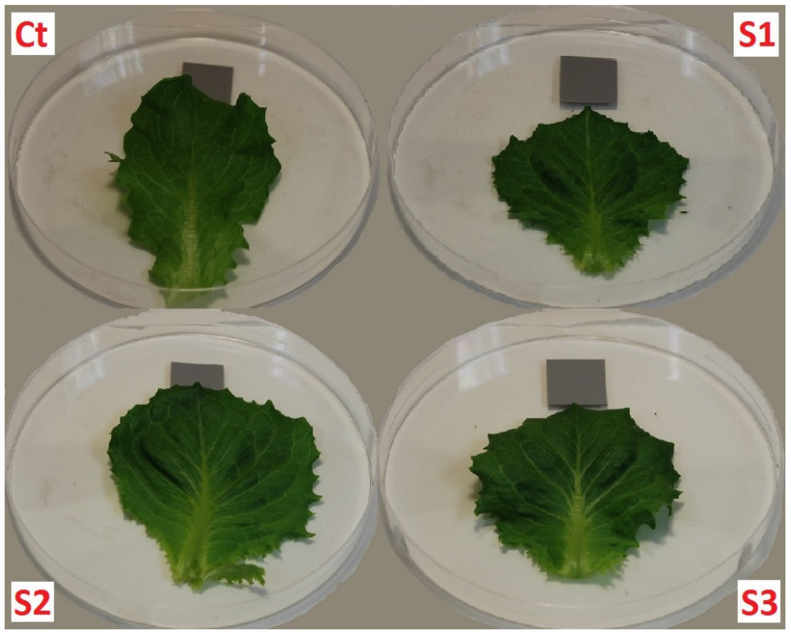
2.1. Materials and Analytical Measurements

The lettuce plants (Lactuca sativa L. var capitata variety “Tempo neutro”) were grown from seeds. The seeds were inserted into polystyrene cylinders that were positioned through holes in the plastic lid of containers with Hoagland´s nutrient solution inside, thus enabling the roots to be in contact with the nutrient solution. The composition of the nutrient solution was 7 mM K+, 4 mM Ca2+, 14 mM NO3, 1 mM Mg2+, 1 mM PO42−, 1 mM SO42−, 20 µM Fe2+, 2.5 µM B3+, 2 µM Mn2+, 2 µM Zn2+, 0.5 µM Cu2+ and 0.5 µM Mo6+; it was maintained between pH levels of 5.5 and 6.5 through routine replacement of the hydroponic solution. After 14 days, plants with similar development were selected and placed in containers (five plants per container) using 15 plants per treatment. Four salt treatments were then applied—a control treatment without NaCl (Ct) and three levels of salt through the addition of different concentrations of NaCl to the nutrient solution: S1 (50 mM NaCl), S2 (100 mM NaCl) and S3 (150 mM NaCl). The application of salt treatments was conducted for a total of 10 days. The average EC of the nutrient solution during the experiments were 1.23 dS/m, 6.09 dS/m, 10.77 dS/m and 14.95 dS/m, for Ct, S1, S2 and S3, respectively. The experiments were performed in a controlled growth chamber with a temperature (T) of 23 °C/18 °C (day/night), a photoperiod of 16 h/8 h (light/darkness) and a photosynthetically active radiation of 400 µmol·m2/s. The leaves were harvested at the end of the experiments and a sample of 10 leaves per treatment, with similar size, was selected for the acquisition of hyperspectral images. Figure 1 shows, as an example, Red-Green-Blue (RGB) images of one leaf per treatment.
After image acquisition, the water content and osmotic potential were determined for the harvested leaves. The leaf water contents were estimated following the method described by [23] with modifications. Twenty grams of leaf pieces per treatment were taken, homogenized with a commercial grinder, and divided into three samples of five grams per treatment. The samples were dried in an oven (Thermocenter T C40/100, Salvis Lab, Rotkreuz, Switzerland), at 65 °C until achieving a constant weight. The water content (WC) was calculated as:
%   W C = Fresh   weight Dry   weight Fresh   weight × 100
For the calculation of the osmotic potential (Ψs), three 5-g samples of leaf pieces per treatment were collected and frozen at −20 °C. The samples were centrifuged at 2800× g (9.8 m/s2) for 15 min (Centronic centrifuge, J.P. Selecta, Barcelona, Spain). The supernatant was analysed with a micro-osmometer (Roebling 13DR, Löser Messtechnik, Berlin, Germany) to determine osmolarity. The osmotic potential was calculated with the Van’t Hoff equation [24]:
Ψs = −R·x·T·x·cs
where R is the ideal gas constant (m3·Pa·mol−1·K−1), T is the temperature (K), and cs is the osmolarity (Osm·m−3).

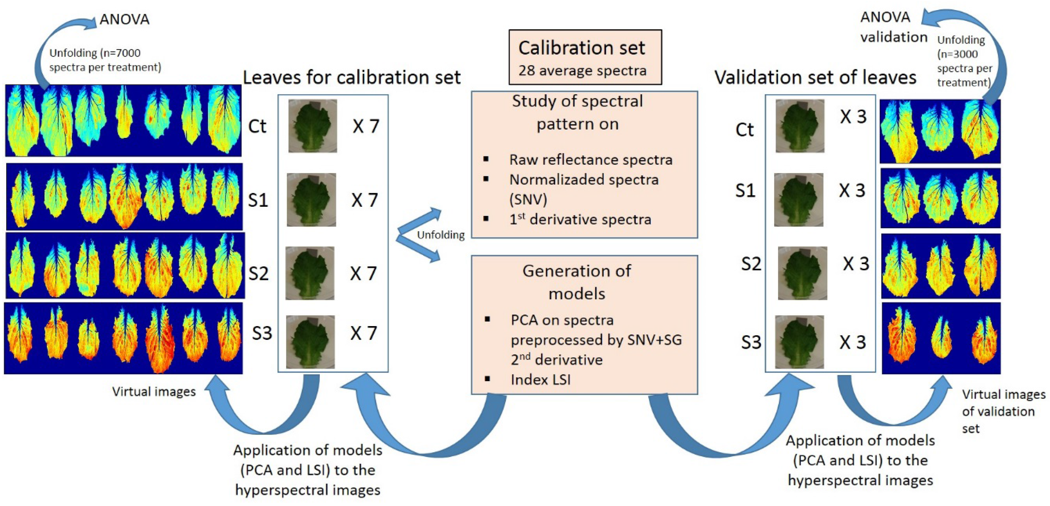
2.2. Hyperspectral Images

Hyperspectral images from the adaxial surfaces of 40 selected leaves were taken with a hyperspectral vision system, consisting of an EMCCD Luca-R camera (Andor™ Technology, Belfast, Northern Ireland) coupled to a VIS-NIR spectrometer (Headwall Photonics Hyperspec-VNIR™, Fitchburg, MA, USA) working in the range of 400–1000 nm. A total of 189 wavelengths were considered along this range, thus obtaining a spectral resolution of 3.2 nm. The spectrometer of the camera was equipped with a progressive line-by-line scan spectrograph with a slit of 25 µm. The spatial resolutions in the line direction and in the scan direction were 0.26 mm/pixel and 0.1 mm/pixel, respectively. A halogen lamp was used for illumination. Headwall Hyperspec™ software (Hyperspec III, Headwall PhotonicsTM, Fitchburg, MA, USA) was used to control the equipment. Samples were scanned by acquiring the entire surface of the leaf (scan length = 100 mm) creating a hypercube dataset. Relative reflectance hyperspectral images were simultaneously computed by the software of the camera. White reference (barium sulfate) and dark current signal (acquired with the objective of the camera covered by a black tap) were acquired before each batch of images. Each line of the image was then corrected pixel by pixel by subtracting the dark current and dividing the result by the white reference minus the dark current.

Data Preprocessing and Processing. Computation of Models

The 40 hyperspectral images of lettuce leaves were randomly divided in two different groups: a calibration set with seven leaves per treatment (28 leaves in total) for generating the models, and a validation set with the three remaining leaves of each treatment (12 leaves in total) for testing the models. Figure 2 shows schematically the procedures carries out for the computation and validation of the models developed.
For each hyperspectral image, the pixels from the green surface of the leaves, eliminating the mid-rib pixels, were considered. The corresponding spectra (a minimum of 32,000 in the smaller leaf) were used to calculate the mean spectrum of each leaf.
The differences on the spectral signature of the spectra was faced analyzing the raw reflectance spectra, the normalized spectra by Standard Normal Variate scaling (SNV) and their corresponding first derivatives, which allow to identify better the displacement left-right of certain bands of the spectrum, such as the red edge area [25,26]. The first derivative of the leaves mean spectra was computed by means of the Savitzky–Golay (SG) algorithm [27]. In the present work, a polynomial of order three was fitted to each spectrum considering 21 wavelengths width to smooth spectra, and then the first derivative function was applied.
For the calibration set, containing the 28 mean spectra, two different preprocessing were applied in order to remove the additive and the multiplicative effect such as it has been previously reported on spinach leaves by [28]. Savitzky–Golay smoothing and differentiation algorithm (SG) was applied to the spectra: a polynomial of order three was fitted considering 21 wavelengths width and the second derivative function was applied to the smoothed spectra (D2). After SG algorithm, the multiplicative effect was corrected by SNV scaling [29]. SNV subtracts to each wavelength of the spectrum (λi) the mean value of this spectrum (λm), and it divides this result by the standard deviation of this spectrum (STD). Therefore resulting spectra have a standard deviation equal to one and a mean equal to zero.
For the set of 28 preprocessed (SG D2 SNV) spectra, a principal component analysis (PCA) was performed in order to obtain an initial model. The loading(s) of the principal component(s) (PC) that showed to be the most sensitive to the effect of the salinity was retained such as the vector of projection (or model) that was applied to the totality of hyperspectral images: those used to compute the average spectra (n = 28 hyperspectral images) of the calibration set, and those that have not been implied at all in the definition of the model and that allow to carry out its external validation (n = 12 hyperspectral images). The hyperspectral images (SG D2 SNV preprocessed) were projected onto the chosen principal component(s) producing the corresponding artificial images of scores.
As a result of these analyses and taken into account the pattern of the loadings obtained in the PCA, an index that computes an approximation to the second derivative at the red edge region was proposed. It was named Level Salinity Index (LSI). This index was also applied to all the hyperspectral images of the leaves (n = 40 hyperspectral images), thus obtaining the corresponding virtual images of the index.
In order to evaluate the ability of the proposed index in comparison to other previously applied, a collection of indexes described in the literature were computed on a representative group of spectra of the calibration set. Only 7000 spectra per treatment (28,000 spectra in total) were considered in order to evaluate the ability of the indexes in a worst scenario, in systems with poorer spatial resolution and consequently lower number of pixels per image. Some of them are specifically related to salinity and others related to water, pigments and chlorophyll content under stress conditions. One-way Analysis of Variance (ANOVA) and Tukey’s least significant difference procedures were carried out for each index comparing the salinity treatments. In addition, scores resulting from PCA of preprocessed spectra was included in such comparison.
Similarly to the procedure followed in the calibration set, in the validation set of virtual images of scores of PCA and of the index proposed in this work, 3000 pixels per treatment were randomly selected and one-way ANOVA’s and Tukey’s least significant difference procedures were applied.
In addition to ANOVA’s, the virtual images (PCA scores and LSI) of the calibration and validation set were also used for comparison, evaluating visually the differences between salinity classes and the spatial distribution of the effects of the salinity on the leaves.
In order to improve the visualization of these virtual images, the pixels of the nerves were not considered. For that a segmentation procedure was applied to the images. Firstly, artificial images were computed based on the combination of planes 730, 680 and 550 nm, where the main differences between nerve and green area were observed. Then the Otsu method was applied to these images to obtain the mask that separated the green areas and the nerves. Finally, these masks were applied onto the scores and index images.

3. Results and Discussion

3.1. Effect of Salinity on Water Content and Osmotic Potential

The water content and osmotic potential data are shown in Table 1. The water content of the leaves decreased when saline concentration increases from 50 mM NaCl to 150 mM NaCl, while similar values were obtained in the control and in the samples subjected to 50 mM NaCl. The same trend can be observed with the osmotic potential of the leaves, but in this parameter distinguishing also between control and 50 mM NaCl, being significantly more negative than control. Salinity increase can induce the accumulation of ions, mainly Na+ and Cl, in the leaves. This fact would be in accordance with the results shown in Table 1, since an accumulation of ions implies a water content reduction and a more negative osmotic potential in the leaves. These results confirm that the salinity levels studied are actually having an effect on the leaves.

3.2. Effect of Salinity on Spectral Features

3.2.1. Non Preprocessed and SNV Reflectance Spectra

The mean spectrum of each saline treatment was computed (calibration set, n = 7 leaves per treatment). The raw spectra and the preprocessed SNV spectra were considered for comparison. Figure 3A shows the mean spectra of each saline treatment. It can be seen that the Ct global reflectance is lower than the others, primarily in the infrared range. This fact can be related to certain physical properties inducing lower scattering in the leaves of the Ct leaf samples.
Crops often have a higher NIR reflectance level under water stress conditions [16,17,18] due to air replacing water between the cells and producing optical discontinuities and scattering. Blum [30] noted that crops under salt stress conditions typically show the same symptoms as under water stress conditions. Salinity affects the osmotic potential of the plants and the water availability of the soil; as such, the water absorption capacity is affected [5]. As shown in Table 1, the osmotic potential and water content in the lettuce leaves decreases when the salinity increases, mainly in S2 and S3 treatments. This fact could induce water stress in the plants that could justify the higher NIR reflectance observed in the leaves of those treatments.
Other effects observed in the crops under saline stress include the loss of growth and turgor, as well as the destruction of cellular membranes [31]. Moreover, an accumulation of salt in the leaves can alter the refractive index of the water. Gitelson et al. [32], the increase in NIR reflectance could be caused by an increase in the thickness and density of the leaves. This fact has been observed in leaves under moderate salinity levels [6]. All of these described effects can affect the scattering process, and this scattering can induce a multiplicative effect on the spectra in the NIR region. This multiplicative effect has been removed applying SNV.
Figure 3B shows the mean spectra of the leaves in each saline treatment corrected with SNV normalization in order to remove the multiplicative effect. Differences among each spectrum can be observed in two areas (Figure 3C): (1) the peak near 550 nm and (2) the valleys near 480 and 680 nm.
The visible region of the spectra depends on the absorbance of the different pigments of the leaves, mainly chlorophyll but also carotenoids and flavonoids. The reflectance peak near 550 nm is due to the significant absorption of chlorophyll in the blue and red regions and the reflection in the green region. The height of the peak of each spectrum can be compared by computing the difference between the reflectance values at 550 and 510 nm. A progressive and systematic decrease in the height of the peak was observed from the Ct to the S3 treatments as the salinity increased. Many authors have related the changes in the visible region of the spectra to the decrease of pigment content in the leaves, primarily of chlorophyll [20,32,33]. When the chlorophyll content decreases, there is an increase of reflectance mainly in the blue and red regions of the spectra. This effect causes the spectra to flatten, resulting in a decrease in the height of the peak near 550 nm. Some research indicates that the total chlorophyll and carotenoid content decreases in plant leaves under salt stress [34]. Gitelson et al. [35] introduced a carotenoid reflectance index (CRI550) (Equation (3)), based on the reflectance values at 510 (R510) and 550 (R550) nm, to follow the evolution of the carotenoid content in the leaves, and that decreases with the decreasing of carotenoids.
CRI550 = (1/R510) − (1/R550)
Applying the CRI550 index to our spectra, a decrease in the carotenoid content could be observed as the salinity increased. The values of CRI were 0.78, 0.74, 0.65 and 0.55, respectively, for our salinity treatments from Ct to S3.
Chlorophyll absorption bands at 480 and 680 nm bands, suffered changes in the reflectance level showing a progressive increase with increasing salt concentrations (Figure 3C). This could indicate a slight loss of chlorophyll in the leaves when the salinity increased.
Different views have been reported regarding the observed changes in the visible range with increasing salinity levels. Some studies related to vegetative growth under salinity conditions showed a decrease in the peak at 550 nm and in the visible region with increased salinity in the plants or soil [14,15], which is consistent with our findings. However, other studies showed either an increase in reflectance in the visible region, primarily near 550 nm [26,36], or no differences in the visible range under salt stress conditions [37].

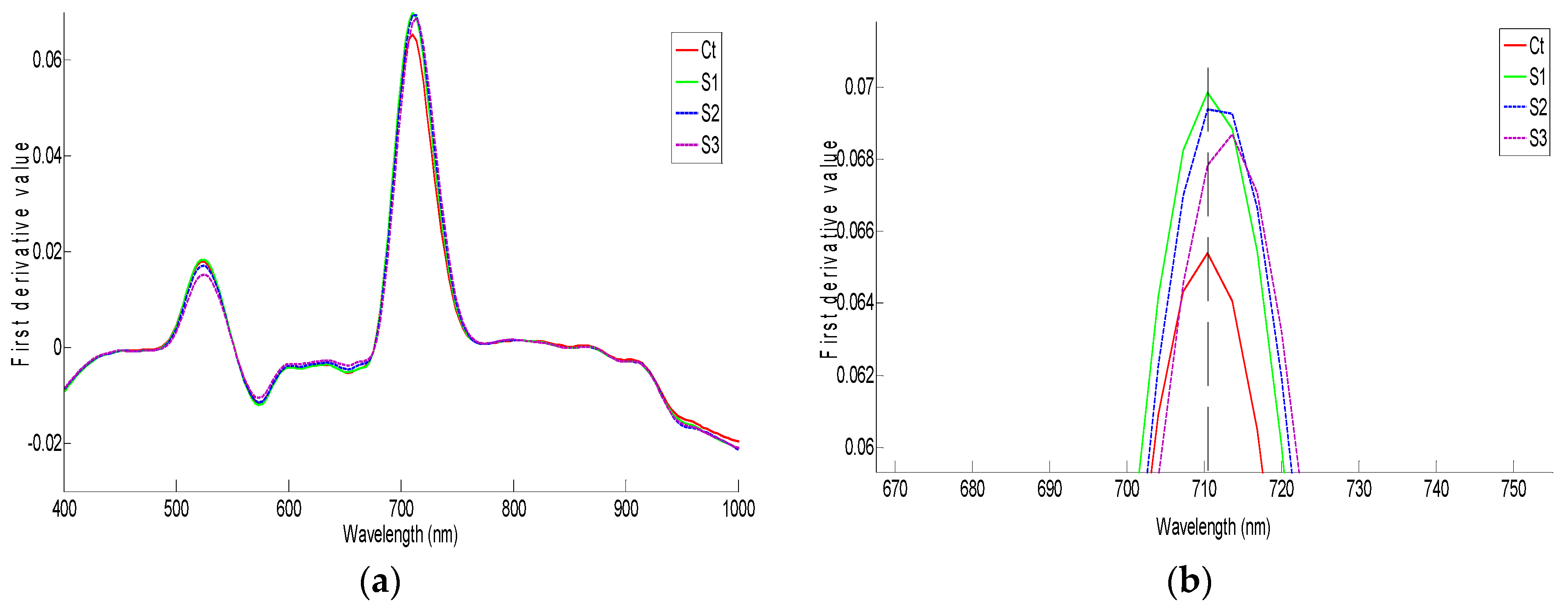
3.2.2. First Derivative of the Spectra

Figure 4A shows the first derivative mean spectra of each saline treatment, where the maximum value corresponds with the red edge. A magnification of the red edge region can be seen in Figure 4B.
A displacement to the right in the peak, though slight and progressive, can be observed in the S3 treatment (Figure 4B). However, numerous authors found that a displacement to the left of the red edge typically occurs when plants suffer environmental conditions of stress (water, nutritive, or salt stress) [21,32,38]. This displacement to the left is typically related to the loss of activity and the degradation of chlorophyll [39]. Lara et al. [28] confirmed this fact in spinach leaves during shelf life and attributed it to aging processes and the loss of cell structure and chlorophyll. However, the effect of aging in harvested leaves over time is not similar to the effect of saline stress in freshly harvested leaves.
Li et al. [26] performed a test with castor bean seedlings under salinity conditions of 0, 100, 200, and 300 mM of NaCl. They observed a displacement to the right of the red edge at 100 mM NaCl and displacements towards the left edge for higher concentrations. This salt concentration (100 mM) is in the range of the highest concentrations of the present research. The salinity may initially cause a displacement of the red edge to the right until reaching a certain level of salt concentration, subsequently shifting to the left when the salinity stress increases; this concurs with [26].
Although it has been reported that an increment in the soil salinity generally tends to induce a decrease in leaf reflectance in the NIR spectral region [40], in this study in that region (800–1000 nm), it can be observed a minimal effect of the salinity. As high near infrared reflectance values are associated with proper development of the plants, it could be interpreted that the levels of salinity applied in the present study are not enough to induce change in the NIR, i.e. are not enough to cause the displacement of the red edge towards lower wavelengths.

3.3. Models and Data Processing

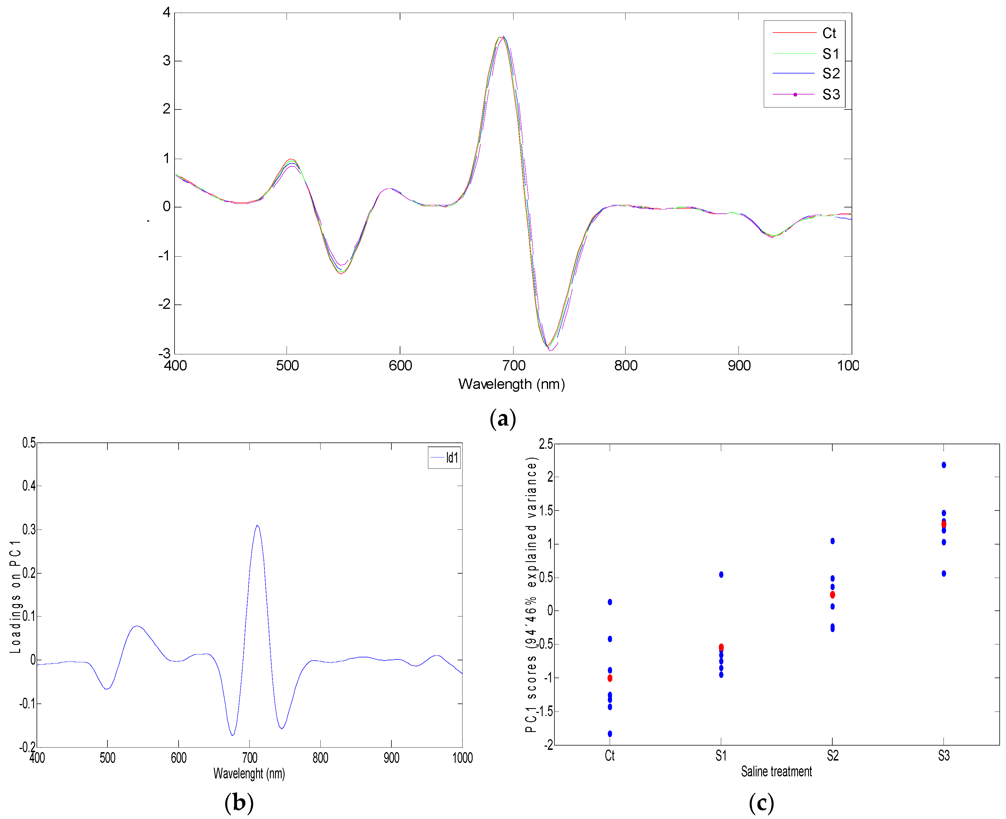
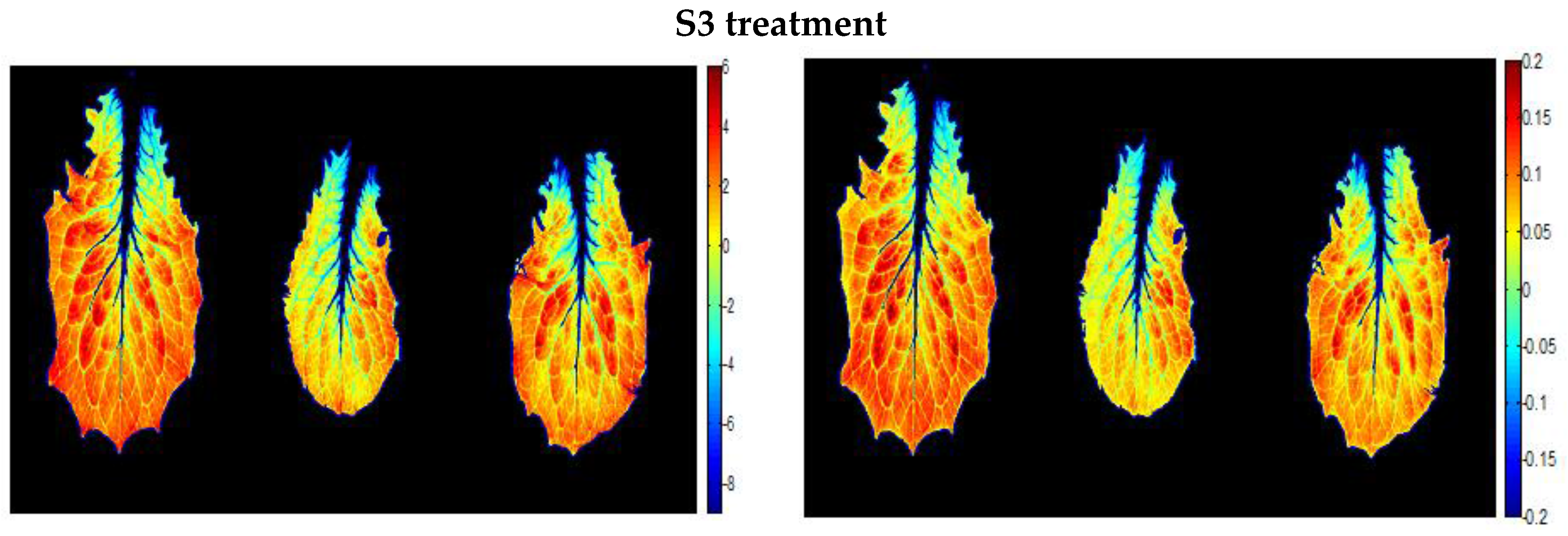
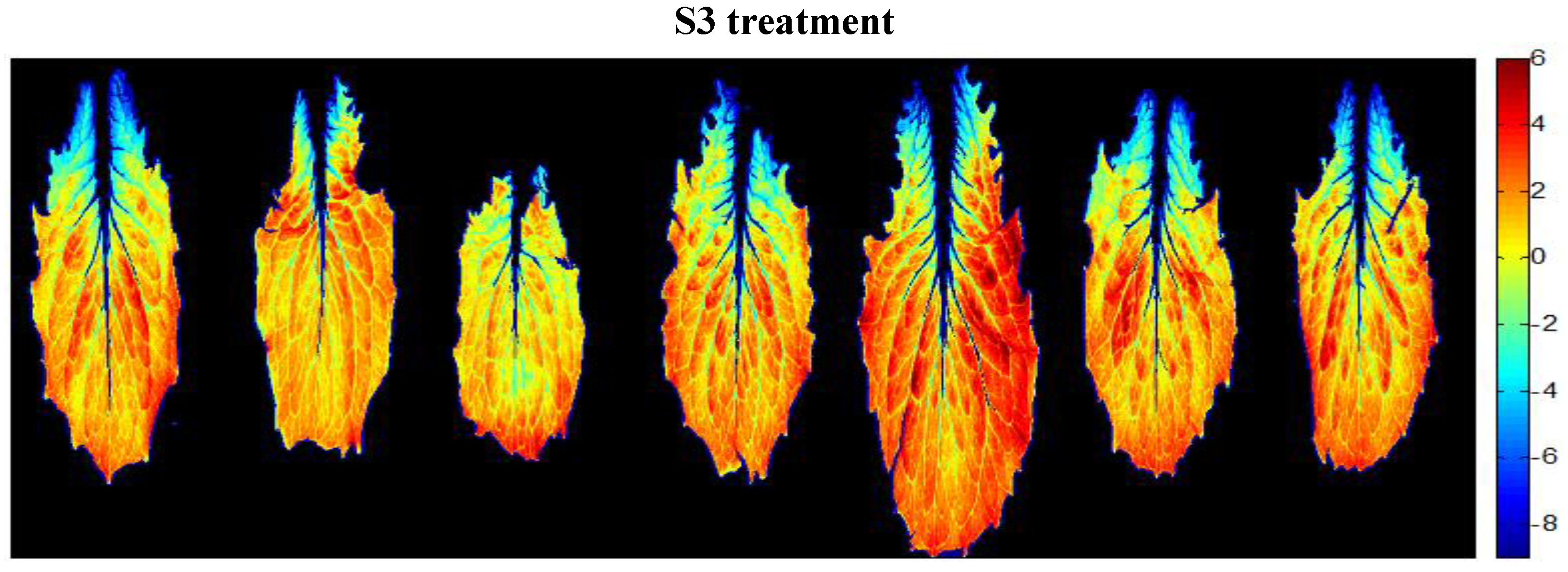
3.3.1. Second Derivative and SNV Normalization: Principal Component Analysis

Figure 5A shows the mean preprocessed spectra (SG D2 SNV) corresponding to the seven leaves from the calibration set for each salt treatment. This preprocessing procedure (SG D2 SNV) showed the best ability for sensing the effect of salinity once PCA was applied, and therefore these spectra were considered for the computation of the PCA model. The second derivative is a measure of the change in the slope of the spectral curve, and therefore it presents a value different from zero when there is a curvature on the spectra. It changes its value if there is a change in the curvature (typically when there is a lateral displacement of the spectra at red-edge area). Just at red edge (maximum slope, inflection point) the curvature is zero, and it becomes different from zero if the spectra move towards the right or towards the left. Peaks at 550 nm and 510 nm in the preprocessed spectra decrease with the salinity level, so the slope of the spectra decrease with increased salinity. This concurs with the previously observed flattening process of the spectra as the salinity level increases.
The first principal component (PC1) from the PCA applied on the SG D2 SNV preprocessed spectra, explaining a 94.46% of variance, was retained as the most related to the changes caused by the salt concentration in the leaves. The PC1 loadings are shown in Figure 5B. The projections of the mean spectra for the PC1 (scores) for each of the four salinity groups are presented in Figure 5C.
Two regions of high loading values can be observed (Figure 5B), corresponding to the major regions with differences in the preprocessed spectra (Figure 5A): one is located at approximately 500–600 nm and the other occurs at the red edge region. The remaining wavelengths have loading values close to zero reflecting no changes in the slope at NIR region, above approximately 780 nm. However, there is an increase of the level of reflectance at this NIR region observed in the raw (without preprocessing) reflectance spectra, Figure 3A. This fact is deeply discussed in Section 3.2.1 and at the end of Section 3.2.2.
The loadings of PC1 around 500–600 nm presents an approximation to the slope between 550 and 510 nm (Figure 5B). Looking to the values (in the loadings of PC1 in the Figure 5B) of “y-axis” at 550 and at 510 nm, it is shown that “y-axis” at 550 is higher and more positive than “y-axis” at 510 (that is negative). Thus, the inner product of PC1 by SG D2 SNV spectra at this region produces an approximation to the slope at this range. As the salinity level increases, the value of the slope (which is negative in this range) increases (because it becomes less negative).
In addition, the SG D2 SNV spectra showed a displacement to the right at the red edge region. PC1 also senses this displacement of the preprocessed spectra at 710 nm. Looking to the PC1 in the region comprises between 675 and 745 nm, the y-axis value at 675 nm and at 745 nm is lower and negative in comparison with y-axis value at 710 nm, which is positive. Therefore, inner product of PC1 by SG D2 SNV spectra at this region produces an approximation to the minus second derivative at 710 (−SD710) [28]:
−SD710 = 2 × R710 − R675 − R745
where −SD710 is related to the curvature at 710 nm: if this wavelength corresponds to the inflection point, the –SD710 is equal to zero; on the contrary, −SD710 will be positive if the preprocessed spectra move towards the right. In the present research the preprocessed spectra at red-edge region moved towards the right, with the increasing levels of salinity, so −SD710 showed increasing values. As a consequence of the above-mentioned facts, the scores of PC1 (i.e., the projection of each spectral signal, in our case the SG D2 SNV spectra, in the PC, obtained multiplying the spectra by the loading) evolved towards higher values showing the behavior described around 500–600 nm and 710 nm.
Scores progressively evolve towards higher values with increasing levels of salinity. Therefore, both previously mentioned regions (500–600 nm and 710 nm) could be related to the salt concentration of the leaves. The analysis of the results of the PCA on the SG D2 SNV spectra allowed identifying similar spectral regions more susceptible to the effect of salinity than the analysis of the SNV spectra and first derivative spectra.
Figure 6 shows the images of scores of the leaves from the calibration set. These images are obtained projecting the hyperspectral images, corrected with SG D2 SNV, on the PC1. The differences between Ct and S3 leaves were clear, evolving from blue pixels (low score value) to orange and red pixels (high score value) when the salinity concentration increased.

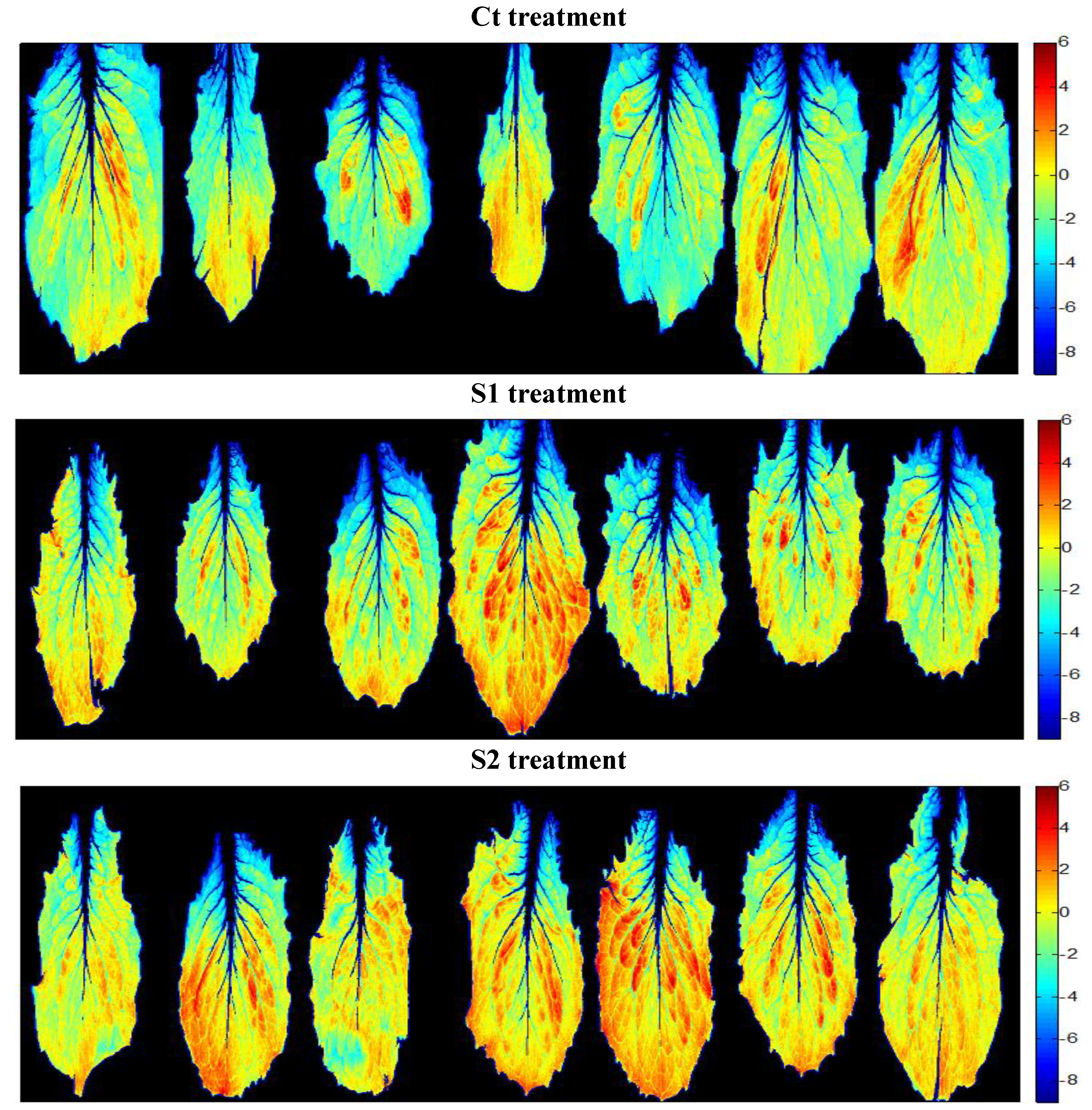
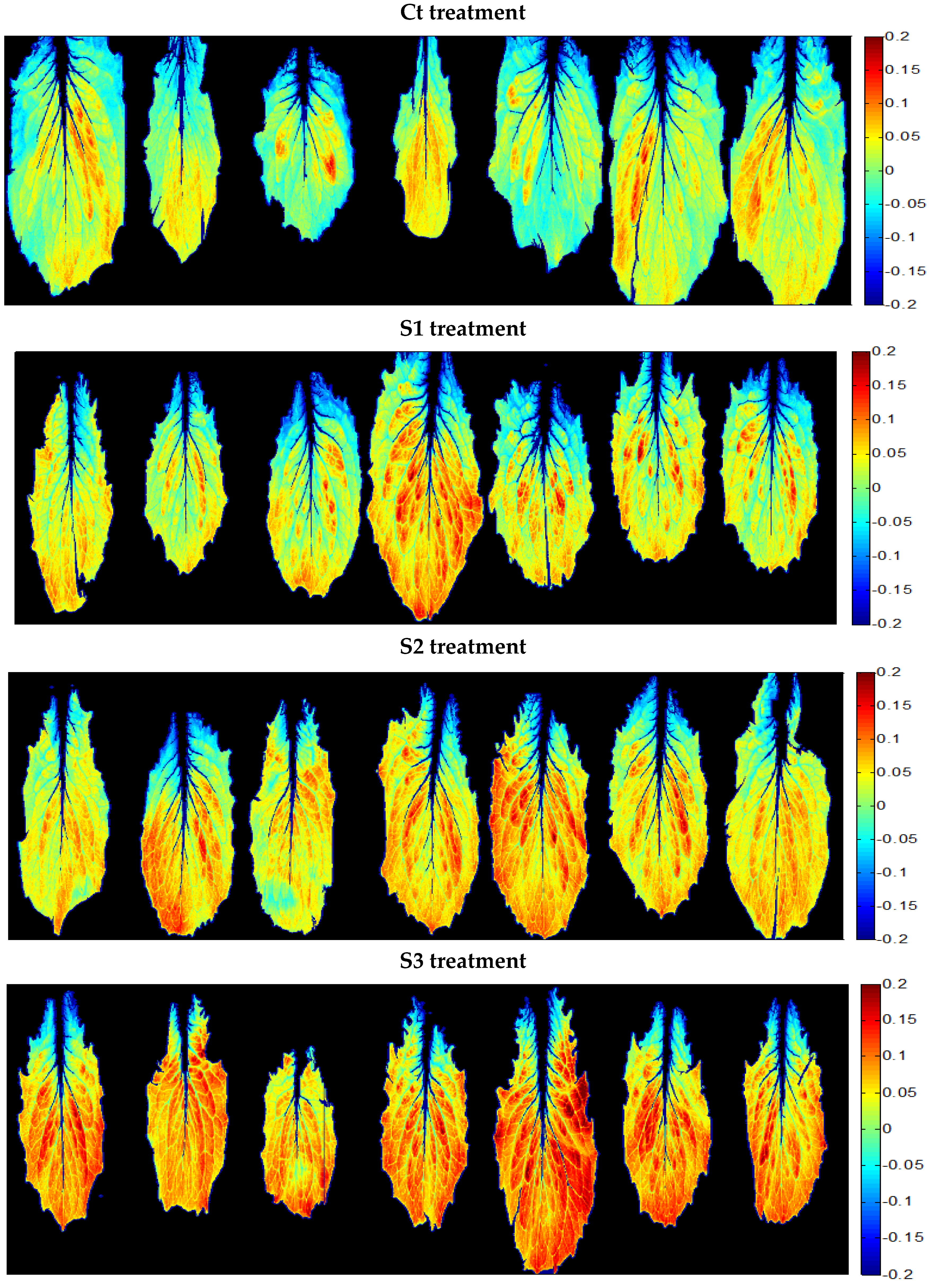
3.3.2. A New Index on the Red Edge Region: Level Salinity Index LSI

A new spectral index (combination of only few wavelengths) was considered for multispectral proposes; they could be cheaper and faster than hyperspectral vision systems. As previously explained, a slight displacement to the right of the red edge region was observed on the first derivative of the spectra of the S3 treatment, which could be related to the moderate increase in the salt concentration of the leaves. On the other hand, the PC1 loading showed the red edge region as the most sensitive area to changes in the spectra induced by salinity. Consequently, an index, Level Salinity Index (LSI), based on the most relevant wavelengths of PC1 loadings (Figure 5B) was proposed.
This LSI index is an approximation to the second derivative at 710 nm (see explanation at Section 3.3.1) and it is a value related to the red edge displacements observed in the SG D2 SNV preprocessed spectra and also in the loadings of PC1. It is also very similar, but not identical, to the proposed by [28]:
LSI = [(R675 + R745)/2] − R710
The LSI was applied to each pixel of the hyperspectral images of the calibration set leaves in order to generate corresponding virtual images and predict the salinity effects on the leaves (Figure 7).
Clear differences between the LSI values from the pixels of the leaves corresponding to the control treatment (Ct) and the pixels of the leaves corresponding to the highest salinity treatment (S3) were observed (Figure 7). The increase in the LSI values noted in the images responds to a lateral displacement of the red edge to the right [28,41], which concurs with the findings obtained from the first derivative spectra analysis.

3.3.3. Comparison between Spectral Indexes

Table 2 presents eleven narrow band indexes that are related to pigment, water content and salinity effects, all of them extracted from a literature review on this topic.
These eleven indexes, along with LSI index and PCA scores, are applied on the spectra of the leaves from the calibration set (n = 1000 spectra per leaf, 7000 spectra per salinity class). Table 3 presents the results of the one-way ANOVA’s and Tukey–Kramer tests performed on these indexes, calculated considering as grouping variable the salinity treatment. LSI (F = 3440.2), Green and Indigo Ratio (GIR) (F = 1340.2), Green region Normalized Difference Vegetation Index (NDVIgreen) (F = 1160.7), Chlred edge (F = 1024.1), NDVI705 (F = 874.2), Chlgreen (F = 737.2), NDVIfar red (F = 702.8) and RPI (F = 686.4) showed consistent trends and all of them were able to distinguish the four groups of salinity treatments. Among these indexes, the three with the highest segregation ability had been specifically defined for sensing salinity effects (LSI, GIR and NDVIgreen). However, Simple Ratio Vegetation Index (SRVI) (F = 119.7), also for salinity detection, together with NDVI (F = 137.3), Plant Senescence Reflectance Index (PSRI) (F = 119.8) and Water Index (WI) (F = 53.4), did not give consistent trend or clear distinction between salinity classes. The scores of PC1 showed similar segregating ability as LSI (F = 2845.88).
Although seven of the eleven indexes reviewed from literature showed good performance for salinity effect detection, the LSI index, specifically defined for images of lettuces acquired under laboratory conditions, exhibited the best behavior, with the highest F-value (Table 3).

3.4. Validation of the Models to Evaluate Salinity Effects

In order to test the performance of the prediction models generated on the calibration set, both models (PC1 on SG D2 SNV spectra and LSI index) were applied to the hyperspectral images of the leaves of the validation set, thus obtaining corresponding virtual images for each case of the two sets. Table 4 presents the results of the one-way ANOVA’s and Tukey–Kramer tests performed on the LSI indexes and PCA scores of n = 1000 spectra from each leaf of the validation set, considering as grouping variable the salinity treatment. Differences between the leaves corresponding to the Ct treatment and the S3 treatment (Figure 8) were observed with both models. It can be seen that the virtual images of both models for the same leaf showed a similar distribution of pixel values. Both types of virtual images were able to sense the effect of salinity in a similar way. However, the LSI-based model was simpler and faster to apply because it is based solely on the reflectance at three different wavelengths.
It can be observed in the images that the pixels from the external parts of the leaves are the most affected by the salinity. The salinity effect is more intense in the areas furthest away from the veins of the leaves. In an intact plant, water is transported to the leaves through the xylem of vascular bundles that branch into a fine network of nerves through the leaf [48]. Salinity restricts water uptake and transpiration and thus reduces water and nutrient uptake and transport to young leaves [49]. This limitation in the xylem transport due to the effect of salinity could explain why the most affected areas of the leaves correspond to areas with thin venation (leaf margin).
As it was introduced, salinity stress can induce marginal necrosis and tip burn in the leaves of lettuce. These symptoms have recently been associated with local oxidative stress in leaf margins that appear before symptom expression [9]. This pattern is coincident with the distribution of the most affected pixels by salinity in our images. Because of this, hyperspectral images could be used to detect symptoms of salt stress in leaves before visible damage expression and thus avoid significant economic losses in crop production.

4. Conclusions

Hyperspectral images were applied in a non-destructive manner to evaluate the effect of salinity on lettuce leaves at harvest. These images were studied in order to determine the best combination of wavelengths for diagnosing the problem of salinity in lettuce leaves.
Based on the spectral features, two models were proposed. The first model was based on a principal component analysis of the second derivative mean spectra of the leaves and normalized with SNV. PC1 was most related to the changes in the leaves induced by salt concentration. By projecting the conveniently processed hyperspectral images on the PC1, the corresponding virtual images of scores showed clear differences among the leaves for each saline treatment.
The second model was based on an LSI index focused on the red edge region. Several indexes from literature exhibited ability to sense the salinity effect on the leaves. However, LSI was the most discriminant index compared to them. This fact could indicate that the detailed interpretation of the spectra behavior could enhance the performance of indexes in each particular cultivar and condition. Once the index is proposed, a less expensive multispectral system could be employed to compute the respective virtual images (only three wavelengths were actually required).
An analysis of variance using only about 1% of pixels extracted at random from the total population of pixels of each leaf showed significant differences between the leaves for each salinity level; in an industrial application, this allows for the implementation of a hyperspectral or multispectral device with smaller spatial resolution. This could simplify the technology, managed data volume and hardware requirements of the system, making it more economical and faster.
Hyperspectral images allow for observations of the distribution of the salinity effects on the surface of the leaves, which are more intense in the areas furthest from the veins. Marginal necrosis appearing in leaves of plants under salinity stress can be detected by the artificial images before the damage is visible.
Further research will be necessary to validate these models with larger data sets and salinity ranges and different varieties and growing conditions than those examined in this study.

Acknowledgments

The funding of this work was supported by the MICINN through projects Multihort (AGL2008-05666-C02-01) and QualityLeaf (AGL2013-48529-R). LPF-TAGRALIA is part of the CEI Moncloa Campus.

Author Contributions

Miguel Ángel Lara, Belén Diezma and Lourdes Lleó conceived and designed the experiments, and wrote the article. Miguel Ángel Lara, Belén Diezma, Lourdes Lleó, Yolanda Garrido and María Isabel Gil performed the experiments. Miguel Ángel Lara analyzed the data. Yolanda Garrido and María Isabel Gil contributed reagents and materials, provided knowledge about plant physiology and reviewed the article. Jean Michel Roger contributed chemometrics tools, provided knowledge in chemometrics and data analysis, and reviewed the article. Margarita Ruiz-Altisent provided scientific knowledge and reviewed the article.

Conflicts of Interest

The authors declare no conflict of interest.

References

  1. Lamsal, K.; Paudyal, G.N.; Saeed, M. Model for assessing impact of salinity on soil water availability and crop yield. Agric. Water Manag. 1999, 41, 57–70. [Google Scholar] [CrossRef]
  2. Shannon, M.C.; Grieve, C.M.; Francois, L.E. Whole-plant response to salinity. In Plant-Environment Interactions; Wilkinson, R.E., Ed.; Marcel Dekker: New York, NY, USA, 1994; pp. 199–244. [Google Scholar]
  3. Acosta, J.A.; Faz, A.; Jansen, B.; Kalbitz, K.; Martínez-Martínez, S. Assessment of salinity status in intensively cultivated soils under semiarid climate, Murcia, SE Spain. J. Arid Environ. 2011, 75, 1056–1066. [Google Scholar] [CrossRef]
  4. Ünlükara, A.; Cemek, B.; Karaman, S.; Erşahin, S. Response of lettuce (Lactuca sativa var. crispa) to salinity of irrigation water. N. Z. J. Crop Horticult. Sci. 2008, 36, 265–273. [Google Scholar]
  5. Yamaguchi, T.; Blumwald, E. Developing salt-tolerant crop plants: Challenges and opportunities. Trends Plant Sci. 2005, 10, 615–620. [Google Scholar] [CrossRef] [PubMed]
  6. Maas, E.V.; Hoffman, G.J. Crop salt tolerance ± current assessment. J. Irrig. Drain. Eng. 1977, 103, 115–134. [Google Scholar]
  7. Bie, Z.; Ito, T.; Shinohara, Y. Effects of sodium sulfate and sodium bicarbonate on the growth, gas exchange and mineral composition of lettuce. Sci. Horticult. 2004, 99, 215–224. [Google Scholar] [CrossRef]
  8. Eraslan, F.; Inal, A.; Savasturk, O.; Gunes, A. Changes in antioxidative system and membrane damage of lettuce in response to salinity and boron toxicity. Sci. Horticult. 2007, 114, 5–10. [Google Scholar] [CrossRef]
  9. Carassay, L.R.; Bustos, D.A.; Golberg, A.D.; Taleisnik, E. Tipburn in salt-affected lettuce (Lactuca sativa L.) plants results from local oxidative stress. J. Plant Physiol. 2012, 169, 285–293. [Google Scholar] [CrossRef] [PubMed]
  10. Winsor, G.; Adams, P. Diagnosis of mineral disorders in plants. In Glasshouse Crops; Robinson, J.B.D., Ed.; Ministry of Agriculture, Fisheries and Food/Agriculture and Fisheries Research Council, HMSO: London, UK, 1987. [Google Scholar]
  11. Poss, J.A.; Grattan, S.R.; Grieve, C.M.; Shannon, M.C. Characterization of leaf boron injury in salt-stressed Eucalyptus by image analysis. Plant Soil 1999, 206, 237–245. [Google Scholar] [CrossRef]
  12. Saure, M.C. Causes of the tipburn disorder in leaves of vegetables. Sci. Horticult. 1998, 76, 131–147. [Google Scholar] [CrossRef]
  13. Poss, J.A.; Russell, W.B.; Grieve, C.M. Estimating yields of salt- and water-stressed forages with remote sensing in the visible and near infrared. J. Environ. Qual. 2006, 35, 1060–1071. [Google Scholar] [CrossRef] [PubMed]
  14. Hamzeh, S.; Naseri, A.A.; AlaviPanah, S.K.; Mojaradi, B.; Bartholomeus, H.M.; Clevers, J.G.P.W.; Behzad, M. Estimating salinity stress in sugarcane fields with spaceborne hyperspectral vegetation indices. Int. J. Appl. Earth Obs. Geoinf. 2013, 21, 282–290. [Google Scholar] [CrossRef]
  15. Zhang, T.; Zeng, S.; Gao, Y.; Ouyang, Z.; Li, B.; Fang, C.; Zhao, B. Using hyperspectral vegetation indices as a proxy to monitor soil salinity. Ecol. Indic. 2011, 11, 1552–1562. [Google Scholar] [CrossRef]
  16. Tucker, C.J. Remote sensing of leaf water content in the near infrared. Remote Sens. Environ. 1980, 10, 23–32. [Google Scholar] [CrossRef]
  17. Harris, A.; Bryant, R.G.; Baird, A.J. Mapping the effects of water stress on Sphagnum: Preliminary observations using airborne remote sensing. Remote Sens. Environ. 2006, 100, 363–378. [Google Scholar] [CrossRef]
  18. Clevers, J.G.P.W.; Kooistra, L.; Schaepman, M.E. Estimating canopy water content using hyperspectral remote sensing data. Int. J. Appl. Earth Obs. Geoinf. 2010, 12, 119–125. [Google Scholar] [CrossRef]
  19. Suárez, L.; Zarco-Tejada, P.J.; González-Dugo, V.; Berni, J.A.J.; Sagardoy, R.; Morales, F.; Fereres, E. Detecting water stress effects on fruit quality in orchards with time-series PRI airborne imagery. Remote Sens. Environ. 2010, 114, 286–298. [Google Scholar] [CrossRef]
  20. Al-Abbas, A.H.; Barr, R.; Hall, J.D.; Crance, F.L.; Baumgardner, M.F. Spectra of normal and nutrient-deficient maize leaves. Agron. J. 1974, 66, 16–20. [Google Scholar] [CrossRef]
  21. Masoni, A.; Ercoli, L.; Mariotti, M. Spectral properties of leaves deficient in iron, sulfur, magnesium, and manganese. Agron. J. 1996, 88, 937–943. [Google Scholar] [CrossRef]
  22. Pacumbaba, R.O., Jr.; Beyl, C.A. Changes in hyperspectral reflectance signatures of lettuce leaves in response to macronutrient deficiencies. Adv. Space Res. 2011, 48, 32–42. [Google Scholar] [CrossRef]
  23. Agüero, M.V.; Ponce, A.G.; Moreira, M.R.; Roura, S.I. Lettuce quality loss under conditions that favor the wilting phenomenon. Postharvest Biol. Technol. 2011, 59, 124–131. [Google Scholar] [CrossRef]
  24. Van’t Hoff, J.H. The role of osmotic pressure in the analogy between solution and gases. Z. Phys. Chem. 1887, 1, 481–508. [Google Scholar] [CrossRef]
  25. Richardson, A.D.; Duigan, S.P.; Berlyn, G.P. An evaluation of noninvasive methods to estimate foliar chlorophyll content. New Phytol. 2002, 153, 185–194. [Google Scholar] [CrossRef]
  26. Li, G.; Wan, S.; Zhou, J.; Yang, Z.; Qin, P. Leaf chlorophyll fluorescence, hyperspectral reflectance, pigments content, malondialdehyde and proline accumulation responses of castor bean (Ricinus communis L.) seedlings to salt stress levels. Ind. Crops Prod. 2010, 31, 13–19. [Google Scholar] [CrossRef]
  27. Savitzky, A.; Golay, M.J.E. Smoothing and differentiation of data by simplified least squares procedures. Anal. Chem. 1964, 36, 1627–1639. [Google Scholar] [CrossRef]
  28. Lara, M.A.; Lleó, L.; Diezma-Iglesias, B.; Roger, J.M.; Ruiz-Altisent, M. Monitoring spinach shelf-life with hyperspectral image through packaging films. J. Food Eng. 2013, 119, 353–361. [Google Scholar] [CrossRef] [Green Version]
  29. Barnes, R.J.; Dhanoa, M.S.; Lister, S.J. Standard normal variate transformation and de-trending of near-infrared diffuse reflectance spectra. Appl. Spectrosc. 1989, 43, 772–777. [Google Scholar] [CrossRef]
  30. Blum, A. Plant Breeding for Stress Environment; CRC Press Inc.: Boca Raton, FL, USA, 1988. [Google Scholar]
  31. Leidi, E.O.; Pardo, J.M. Tolerancia de los cultivos al estrés salino: Qué hay de nuevo. Revista de Investigaciones de la Facultad de Ciencias Agrarias 2002, UNR 2, 70–91. [Google Scholar]
  32. Gitelson, A.; Viña, A.; Arkebauer, T.J.; Rundquist, D.C.; Keydan, G.; Leavitt, B. Remote estimation of leaf area index and green leaf biomass in maize canopies. Geophys. Res. Lett. 2003, 30, 1248. [Google Scholar] [CrossRef]
  33. Knipling, E.B. Physical and physiological basis for the reflectance of visible and near-infrared radiation from vegetation. Remote Sens. Environ. 1970, 1, 155–159. [Google Scholar] [CrossRef]
  34. Parida, A.K.; Das, A.B. Salt tolerance and salinity effects on plants: A review. Ecotoxicol. Environ. Saf. 2005, 60, 324–349. [Google Scholar] [CrossRef] [PubMed]
  35. Gitelson, A.; Zur, Y.; Chivkunova, O.B.; Merzlyak, M.N. Assessing carotenoid content in plant leaves with reflectance spectroscopy. Photochem. Photobiol. 2002, 75, 272–281. [Google Scholar] [CrossRef]
  36. Peñuelas, P.; Isla, R.; Filella, I.; Araus, J.L. Visible and near infrared reflectance assessment of salinity effects on barley. Crop Sci. 1997, 37, 198–202. [Google Scholar] [CrossRef]
  37. Wang, D.; Wilson, C.; Shannon, M.C. Interpretation of salinity and irrigation effects on soybean canopy reflectance in visible and near-infrared spectrum domain. Int. J. Remote Sens. 2002, 23, 811–824. [Google Scholar] [CrossRef]
  38. Mariotti, M.; Ercoli, L.; Masoni, A. Spectral properties of iron deficient corn and sunflower leaves. Remote Sens. Environ. 1996, 58, 282–288. [Google Scholar] [CrossRef]
  39. Ustin, S.L.; Gitelson, A.A.; Jacquemoud, S.; Schaepman, M.; Asner, G.P.; Gamon, J.A.; Zarco-Tejada, P. Retrieval of foliar information about plant pigment systems from high resolution spectroscopy. Remote Sens. Environ. 2009, 113, S67–S77. [Google Scholar] [CrossRef] [Green Version]
  40. Peñuelas, J.; Pinol, J.; Ogaya, R.; Filella, I. Estimation of plant water concentration by the reflectance water index wi (r900/r970). Int. J. Remote Sens. 1997, 18, 2869–2875. [Google Scholar] [CrossRef]
  41. Diezma, B.; Lleó, L.; Roger, J.M.; Herrero-Langreo, A.; Lunadei, L.; Ruiz-Altisent, M. Examination of the quality of spinach leaves using hyperspectral imaging. Postharvest Biol. Technol. 2013, 85, 8–17. [Google Scholar] [CrossRef]
  42. Tucker, C.J. Red and photographic infrared linear combinations for monitoring vegetation. Remote Sens. Environ. 1979, 8, 127–150. [Google Scholar] [CrossRef]
  43. Gitelson, A.; Merzlyak, M.N. Spectral reflectance changes associated with autumn senescence of Aesculus hippocastanum L. and Acer platanoides. Leaves spectal features and relation to chlorophyll estimation. J. Plant Physiol. 1994, 143, 286–292. [Google Scholar] [CrossRef]
  44. Gitelson, A.; Merzlyak, M.N.; Lichtenthaler, H.K. Detection of red edge position and chlorophyll content by reflectance measurements near 700 nm. J. Plant Physiol. 1996, 148, 501–508. [Google Scholar] [CrossRef]
  45. Gitelson, A.A.; Keydan, G.P.; Merzlyak, M.N. Three-Band Model for Non-Invasive Estimation of Chlorophyll Carotenoids and Anthocyanin Contents in Higher Plant Leaves. Papers in Natural Resources. 2006. Paper 258. Available online: http://digitalcommons.unl.edu/natrespapers/258 (accessed on 1 November 2016).
  46. Merzlyak, M.N.; Gitelson, A.A.; Chivkunova, O.B.; Rakitin, V.Y. Non-destructive optical detection of pigment changes during leaf senescence and fruit ripening. Physiol. Plant. 1999, 106, 135–141. [Google Scholar] [CrossRef]
  47. Rud, R.; Shoshany, M.; Alchanatis, V. Spectral indicators for salinity effects in crops: A comparison of a new green indigo ratio with existing indices. Remote Sens. Lett. 2011, 2, 289–298. [Google Scholar] [CrossRef]
  48. Holbrook, N.M. El balance hídrico de las plantas. In Fisología Vegetal; Taiz, L., Zeiger, E., Eds.; Universitat Jaume I: Castelló de la Plana, Spain, 2006; pp. 79–115. [Google Scholar]
  49. Lazof, D.B.; Bernstein, N. Effects of salinization on nutrient transport to lettuce leaves: Consideration of leaf developmental stage. New Phytol. 1999, 144, 85–94. [Google Scholar] [CrossRef]
Figure 1. Red-Green-Blue (RGB) image of one leaf per saline treatment. Apparently, no visible symptoms of stress can be observed.
Applsci 06 00412 g001
Figure 2. Scheme of the methodology followed for the computation and validation of both models developed.
Applsci 06 00412 g002
Figure 3. (a) Mean relative reflectance spectra of the leaves of each saline treatment. Calibration set, n = 28 leaves (4 saline treatments × 7 leaves). (b) Same spectra corrected with Standard Normal Variate (SNV) normalization to eliminate multiplicative effect. (c) Zoom in the visible range of SNV corrected spectra. See Table 1 for abbreviations.
Applsci 06 00412 g003
Figure 4. (a) First derivative mean spectra of the leaves of each saline treatment. Calibration set, n = 28 leaves (4 saline treatments × 7 leaves); (b) zoom on the red edge. See Table 1 for abbreviations.
Applsci 06 00412 g004
Figure 5. (a) Mean Savitzky-Golay algorithm (SG), second derivative (D2) and SNV pre-treated spectra of the leaves of calibration set for each saline treatment; (b) The first principal component (PC1) loadings from principal component analysis (PCA) applied on second derivative and SNV processed spectra; and (c) PC1 scores of mean spectra of the leaves of calibration set for each saline treatment (Ct, S1, S2 and S3 treatments, x-axis), with the mean values of each group are shown in red.
Applsci 06 00412 g005
Figure 6. Virtual images of scores obtained by projection of the hyperspectral images, corrected with second derivative Savitzky–Golay algorithm and SNV normalization, on PC1. Leaves from calibration set. Pixels colored from blue to red are showing increasing levels of salinity affectation.
Applsci 06 00412 g006aApplsci 06 00412 g006b
Figure 7. Virtual images obtained by applying the Level Salinity Index (LSI) on each pixel of the hyperspectral images of lettuce leaves, from calibration set. Pixels colored from blue to red are showing increasing levels of salinity affectation.
Applsci 06 00412 g007
Figure 8. Virtual images obtained by applying both models developed on the hyperspectral images of lettuce leaves, from the validation set. Pixels colored from blue to red are showing increasing levels of salinity affectation. Left: PC1 model. Right: LSI model.
Applsci 06 00412 g008aApplsci 06 00412 g008b
Table 1. Water content and osmotic potential of the lettuce leaves treated without NaCl (Ct) and treated with 50, 100 and 150 mM NaCl (S1, S2 and S3, respectively). Letters indicate the different mean groups according to Tukey’s test for a p level of 0.05.
Saline TreatmentWater Content (%)Osmotic Potential (MPa)
Mean ± STDMean ± STD
Ct94.53 ± 0.09a−0.65 ± 0.04a
S194.54 ± 0.12a−1.08 ± 0.09b
S293.15 ± 0.18b−1.49 ± 0.11c
S392.70 ± 0.07c−2.06 ± 0.09d
Table 2. Indexes used for comparison with Level Salinity Index (LSI) index.
IndexFormula
NDVI, related to chlorophyll content [42]NDVI = (R800 − R670)/(R800 + R670)
NDVI705, related to chlorophyll content [43]NDVI705 = (R750 − R705)/(R750 + R705)
Red Edge Position Index, related to chlorophyll content [44]RPI = (R750/R700)
Related to chlorophyll content in anthocyanin free leaves [45]Chlgreen = (R760/R550) − 1
Chlred edge = (R760/R705) − 1
Plant Senescence Reflectance Index [46]PSRI = (R680 − R500)/(R750)
Water Index, related to water content [40]WI = (R900/R970)
Green region NDVI, related to salinity [13]NDVIgreen = (R550 − R670)/(R550 + R670)
Far red region NDVI, related to salinity [13]NDVIfar red = (R710 − R670)/(R710 + R670)
Simple Ratio Vegetation Index, related to salinity [37]SRVI = (R830/R660)
Green and Indigo Ratio, related to salinity [47]GIR = (R436/R554)
Table 3. Analysis of variance (F-Fisher and p-value) comparing the values of indexes for the four salinity classes (n = 7000 spectra per class belonging to the calibration set of leaves). Mean values and standard error of the different indexes per salinity class. Means followed by the same letter are not significantly different by Tukey–Kramer test; different letters implies there is significant difference between means.
IndexF-Fisherp-ValueMeanStandard Error
LSI3440.20Ct0.01765a0.00045
S10.03130b0.00045
S20.05175c0.00045
S30.07829d0.00045
NDVI137.32.45 × 10−88Ct0.82469a0.00080
S10.80969b0.00080
S20.80345c0.00080
S30.80714d0.00080
NDVI705874.20Ct0.45693a0.00076
S10.46466b0.00076
S20.47856c0.00076
S30.50774d0.00076
RPI686.40Ct3.48135a0.00864
S13.54853b0.00864
S23.64758c0.00864
S33.99075d0.00864
Chlgreen737.20Ct2.26632a0.00731
S12.28408a0.00731
S22.39855b0.00731
S32.69576c0.00731
Chlred edge1024.10Ct1.78446a0.00583
S11.84552b0.00583
S21.94359c0.00583
S32.20687d0.00583
PSRI119.84.38 × 10−77Ct−0.00536a0.00013
S1−0.00706b0.00013
S2−0.00552a0.00013
S3−0.00366c0.00013
WI53.42.03 × 10−34Ct1.28100a0.00036
S11.27616b0.00036
S21.27872c0.00036
S31.28220d0.00036
NDVIgreen1160.70Ct0.53842a0.00108
S10.50228b0.00108
S20.47366c0.00108
S30.45415d0.00108
NDVIfar red702.80Ct0.68830a0.00102
S10.65912b0.00102
S20.63788c0.00102
S30.62661d0.00102
SRVI119.75.35 × 10−77Ct10.53830a0.04345
S19.64646b0.04345
S29.46616c0.04345
S310.04068d0.04345
GIR1340.20Ct0.35211a0.00100
S10.38783b0.00100
S20.41381c0.00100
S30.43755d0.00100
Scores PC12845.880Ct−1.0902a0.000227
S1−0.6474b0.000228
S20.0851c0.000199
S31.1235d0.000212
Table 4. Analysis of variance (F-Fisher and p-value) comparing the values of LSI index and the first principal component (PC1) scores for the four salinity classes (n = 3000 spectra per class belonging to the validation set of leaves). Mean values and standard error of the different indexes per salinity class. Means followed by the same letter are not significantly different by Tukey–Kramer test; different letters implies there is significant difference between means.
IndexF-Fisherp-ValueMeanStandard Error
LSI1491.570Ct0.018450.00131a
S10.031490.00127b
S20.052500.00127c
S30.080180.00127d
Scores PC11197.020Ct−1.053830.05122a
S1−0.632520.05122b
S20.126810.05122c
S31.169110.05122d

