A Novel Personalized Diagnosis Methodology Using Numerical Simulation and an Intelligent Method to Detect Faults in a Shaft

Abstract

Personalized medicine is a hot topic to develop a medical procedure for healthcare. Motivated by molecular dynamics simulation-based personalized medicine, we propose a novel numerical simulation-based personalized diagnosis methodology and explain the fundamental procedures. As an example, a personalized fault diagnosis method is developed using the finite element method (FEM), wavelet packet transform (WPT) and support vector machine (SVM) to detect faults in a shaft. The shaft unbalance, misalignment, rub-impact and the combination of rub-impact and unbalance are investigated using the present method. The method includes three steps. In the first step, Theil’s inequality coefficient (TIC)-based FE model updating technique is employed to determine the boundary conditions, and the fault-induced FE model of the faulty shaft is constructed. Further, the vibration signals of the faulty shaft are obtained using numerical simulation. In the second step, WPT is employed to decompose the vibration signal into several signal components. Specific time-domain feature parameters of all of the signal components are calculated to generate the training samples to train the SVM. Finally, the measured vibration signal and its components decomposed by WPT serve as a test sample to the trained SVM. The fault types are finally determined. In the simulation of a simple shaft, the classification accuracy rates of unbalance, misalignment, rub-impact and the combination of rub-impact and unbalance are 93%, 95%, 89% and 91%, respectively, whereas in the experimental investigations, these decreased to 82%, 87%, 73% and 79%. In order to increase the fault diagnosis precision and general applicability, further works are continuously improving the personalized diagnosis methodology and the corresponding specific methods.

1. Introduction

Rotating machinery has been widely used in transmission machinery, and its running state directly affects the entire machine, including reliability and stability. Thus, the fault diagnosis of the rotating machinery is increasingly having attention paid. Over the past several decades, new fault detection methods [1,2,3,4,5,6,7] and new criteria [8,9,10] were proposed, which greatly enriched the field of fault diagnosis. He et al. [11] proposed a data mining-based diagnostic system using acoustic emission (AE) signals to detect faults in full ceramic bearings. They further developed a series of methods to identify faults in plastic bearings [12], gearbox tooth cut faults [13], planetary gearbox faults [14], etc.

For the fault detection of the shaft, various researchers have reported feasible methods. Mohammed et al. [15] investigated a novel route using artificial neural networks (ANN) and power spectral density (PSD) to detect the cracks in a rotating shaft. As is well known, intelligent methods play an important role in detecting faults in mechanical components, such as genetic algorithms (GAs), neural networks (NNs), support vector machine (SVM), etc., and those approaches have been applied to detect faults using experimental samples of all kinds of faults [7]. However, for the lack of suitable training samples that represent every possible fault in all kinds of practical mechanical systems, the above intelligent techniques have not been agreeable applied to detect faults in mechanical systems.

In order to understand the fault effects in depth, many researchers proposed numerical simulation for fault diagnosis. Torkaman et al. [16] adopted the three-dimensional time-step finite element method (3D-TSFEM) to simulate the fault of a switched reluctance motor (SRM), and the new diagnosis index associated with power losses was obtained in their results. To detect faults online in nonlinear continuous systems, Bregon et al. [17] used the simulation and state observer models to obtain the final fault diagnosis results. Gong et al. [18] investigated rotor dynamic stability analysis on the hydraulic turbine by numerical simulation and also demonstrated how each factor affects the dynamic character of the labyrinth system. Xiang et al. [19,20] carried out two kinds of wavelet-based numerical simulation models to calculate the dynamic responses of a shaft. Tannous et al. [21] performed rotor-stator contact simulations using 3D numerical modeling. Baccarini et al. [22] proposed a dynamic numerical model to simulate mechanical faults in induction machines, and the simulation results confirmed the validity of the model. For numerical simulation, on the one hand, less time and equipment are used to get a large amount of experimental data, especially for those that are very difficult to conduct in a real machine for carrying out the experimental investigation. On the other hand, this allows the investigator to determine the fault samples for all types of faults under the complex running conditions.

In order to perform the intelligent methods, the selection of feature vectors is one of the key problems. Recently, time domain or time frequency domain feature indexes were adopted to create feature vectors. Chen et al. [23] proposed an approach that has six indexes (e.g., mean value, root mean square, standard deviation, skewness, kurtosis and shape indicator) in the time domain and two indexes (e.g., mean frequency and standard deviation frequency) in the frequency domain to construct the feature sets to train the SVM. Liu et al. [24] used a hybrid time frequency analysis method to get the feature information of gear faults.

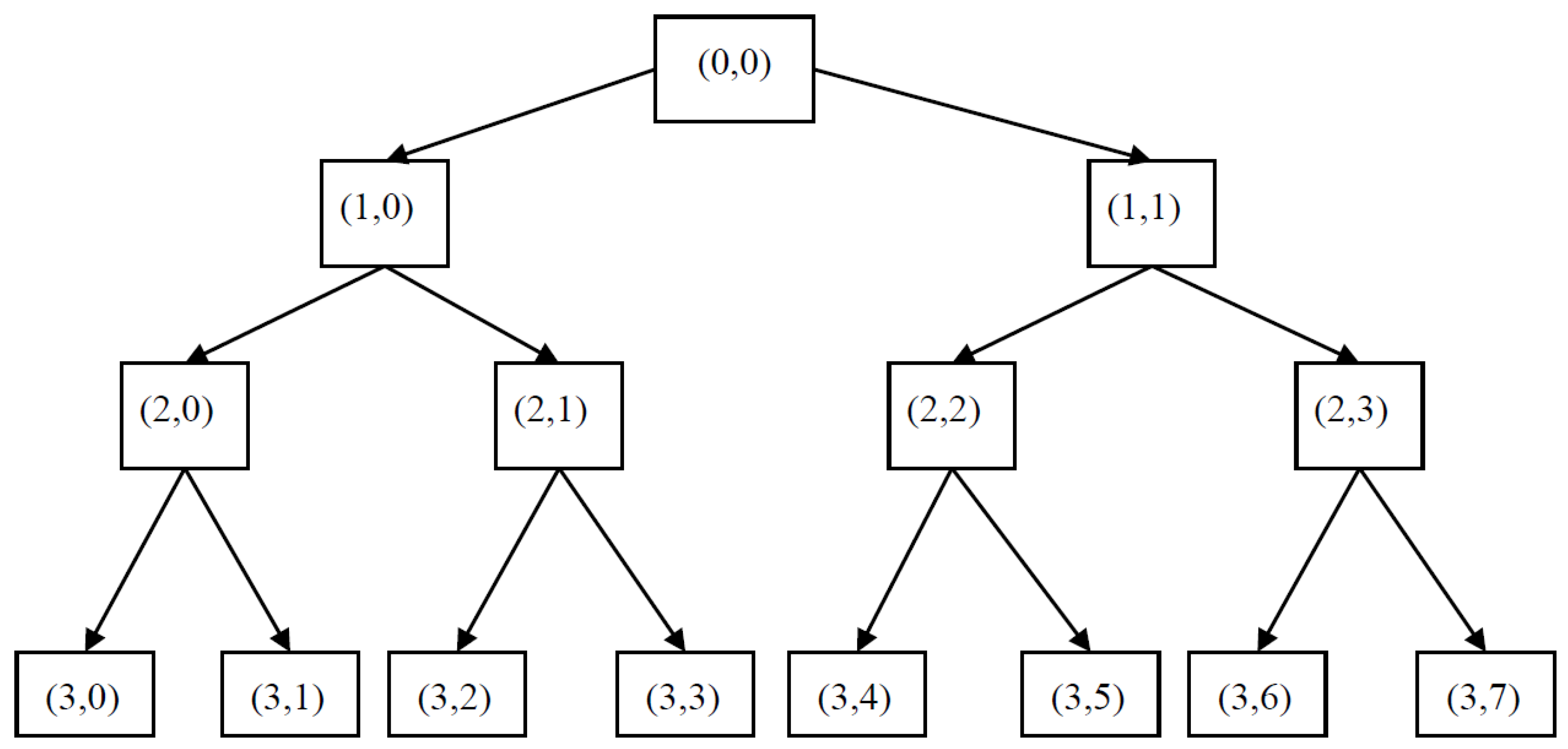
Wavelet packet transform (WPT) is a useful tool in handling non-stationary signals to detect faults in mechanical systems [25]. As a signal processing tool, WPT decomposes the original signal into multi-layers, and the same frequency bandwidth is offered in each layer. Xiang et al. [26] propose a new method based on the wavelet transform for the detection of damages in plate-like and shell-like structures. Diego and Barros [27] employed WPT to analyze the magnitude of the harmonic distortion and the corresponding sub-harmonics in power systems. Pan et al. [28] proposed a novel approach based on improved WPT and support vector data description (SVDD) to assess bearing performance degradation.

To obtain the features of the ignition pattern, Vong and Wong [29] used WPT to decompose the engine ignition signal and then employed multi-class least squares SVM to classify the fault types. It is worth pointing out the coefficients of WPT and the corresponding single branch reconstruction signals on all of the decomposing levels, which play a key role in singularity detection and feature extraction.

As a novel pattern recognition approach, support vector machine (SVM), was proposed in the 1990s by Cortes and Vapnik, and now, it has been widely used in fault classification [30]. The basic theory for SVM is structural risk minimization (SRM) with small training samples, which are suitable for the classification and regression of the nonlinear and high dimensional problems. However, the lack of faulty training samples has greatly limited the fault classification using SVM in real-world applications.

Recently, personalized medicine has become a hot topic to develop a medical procedure that separates patients into different groups, with medical decisions, practices, interventions and/or products being tailored to the individual patient based on his/her predicted response or risk of disease [31]. It is also a new direction for placing the patient at the center of healthcare, and the theoretical basis is molecular dynamics simulation from person to person [32]. Motivated by molecular dynamics simulation-based personalized medicine, the fault detection strategy for mechanical systems might be developed for the personalized diagnosis era. The most probable tools might be numerical simulation, the big data technique or a combination of the two.

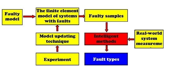
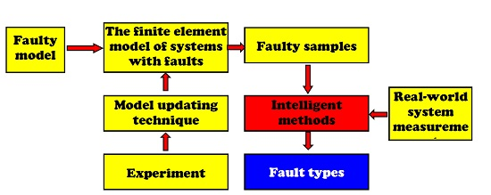
From the above descriptions, it might be concluded that if the limitation of faulty training samples can be inexpensively overcome by numerical simulation using the dynamic model of mechanical systems, the intelligent methods, such as SVM, GAs and NNs, will be directly applied to detect faults for machines under all kinds of working conditions. In this paper, we present the basic idea of a new personalized fault diagnosis methodology focused on the fault diagnosis of shafts. Based on the present methodology, this paper is arranged as follows: The basic idea and the procedures of the personalized diagnosis methodology are presented in Section 2. 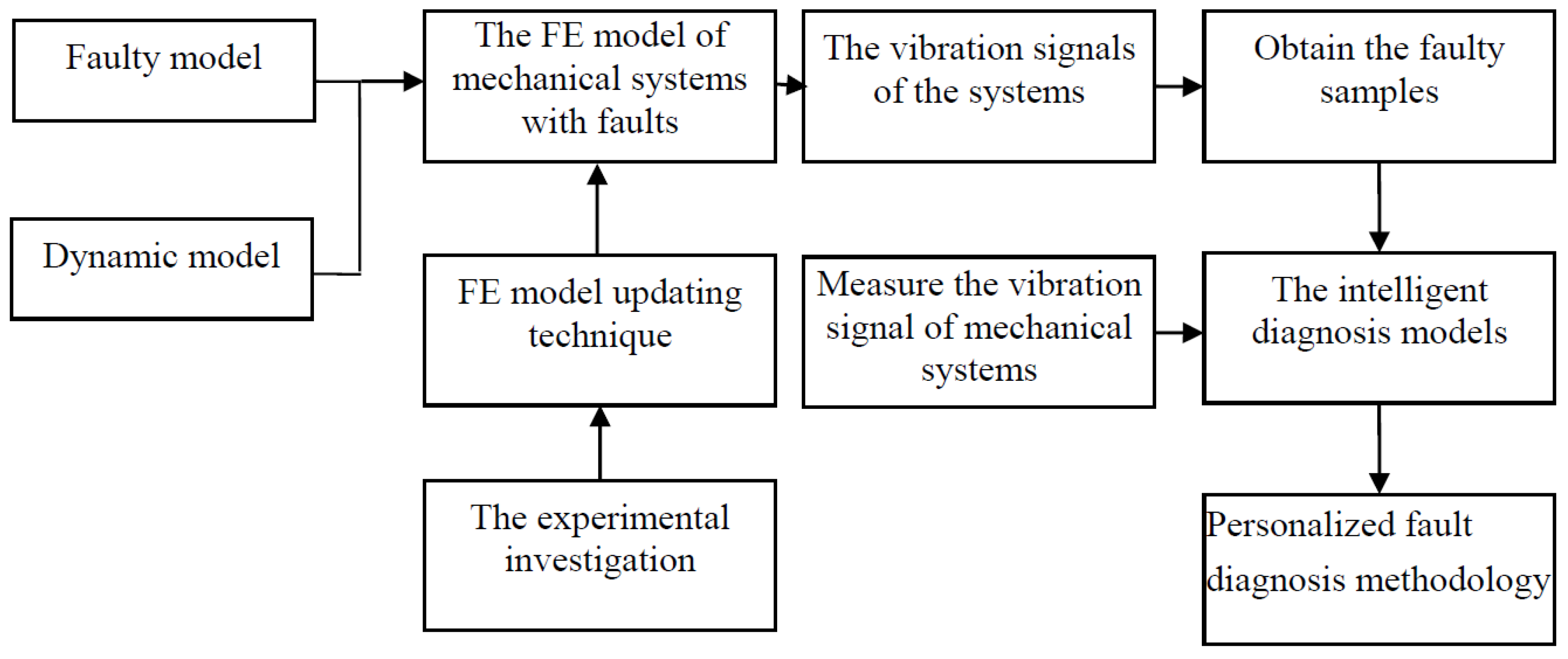In Section 3, finite element (FE) models of shafts are constructed; an example is presented; and the shaft unbalance, misalignment, rub-impact and the combination of rub-impact and unbalance are considered. To further apply the present method to real-world usage, the experimental investigations and further works are discussed in Section 4. Finally, the conclusion of this study is given in Section 5.

2. The Personalized Diagnosis Methodology

2.1. The Basic Idea for the Personalized Diagnosis Methodology

Personalized medicine is a kind of accurate diagnosis technology based on individual differences with the development of molecular biology in recent years [33], which provides a new idea for condition monitoring and fault diagnosis in mechanical systems. Recently, the intelligent diagnosis methods have become one of the hot and promising research areas [34]. The valuable application of intelligent methods has reflected and provided the realization of personalized fault diagnosis in mechanical systems. The early development of mechanical diagnosis and condition monitoring was based on the faulty samples extracted from actual faults in mechanical systems. However, for the complex mechanical system and complicated fault mechanism, there are too many complexity vibration signals to be analyzed. Furthermore, in many faulty cases, it is very difficult to obtain all of the faulty samples when the machine is running. Therefore, the lack of faulty samples will lead to the failure to detect faults in real-world mechanical systems.

Recently, it has been possible to conduct a simulation model of a mechanical system with faults, such as shafts in a rotor-bearing system, bearings and gears in a gearbox, etc., to obtain the faulty samples with various faults of different types using numerical simulation.

Based on the above technique development, the personalized diagnosis methodology is proposed, and the fundamental procedure is shown in Figure 1. In order to realize personalized diagnosis, the present methodology combines the numerical simulation model and intelligent diagnosis methods to detect faults in mechanical systems. Numerical simulation plays a key role in the present methodology to obtain the simulated faulty samples to replace the measured ones. Therefore, the damage location prediction procedure is as follows:

(1) Construct the FE model of mechanical systems with faults:

In the simulation, the faulty model (e.g., unbalance, misalignment, rub-impact, damages, etc.) and the dynamic model of the mechanical system are constructed using finite element method (FEM). To decrease the difference between the measured vibration signals and the computed (by the FE model) ones of the same mechanical systems, the FE model updating technique using the experimental investigation of the intact mechanical systems [35] should be applied to reduce the difference. After the updating process, the resulting FE model of the mechanical systems with faults can be used to calculate the simulation vibration signals.

(2) Obtain the faulty samples:

The FE model of the mechanical systems with faults is calculated for the vibration signal in the time domain. The WPT is then applied to decompose the original vibration signals into multi-layers, and the corresponding sub-signals (components) are finally obtained. To generate the faulty training samples, the time domain indexes, such as the standard deviation (SD), peak, kurtosis, clearance factor (CF), impulse factor (IF), etc. (summarized in

Table 1. Five time domain feature parameters ¹.

Feature	Equation
Standard deviation $x_{\mathrm{std}}$	$x_{\mathrm{std}}=\sqrt{\frac{{{\displaystyle {\sum }_{n=1}^N(x(n)-x_m)}}^2}{N}}$
Peak $x_{\mathrm{p}}$	$x_{\mathrm{p}}=\max \left|x(n)\right|$
Kurtosis $x_{\mathrm{kur}}$	$x_{\mathrm{kur}}=\frac{1}{N}{{\displaystyle {\sum }_{n=1}^N(\frac{x(n)-x_m}{{\mathsf{\sigma }}_{\mathrm{s}}})}}^4$
Clearance factor $CLF$	$CLF=\frac{x_{\mathrm{p}}}{{\left(\frac{1}{N}{\displaystyle {\sum }_{n=1}^N\sqrt{\left|x(n)\right|}}\right)}^2}$
Impulse factor $IF$	$IF=\frac{x_{\mathrm{p}}}{\frac{1}{N}{\displaystyle {\sum }_{n=1}^N\left|x(n)\right|}}$

¹ x is the data; N is the number of data points; x_m is the mean value of x; ${\mathsf{\sigma }}_{\mathrm{s}}$ is the standard deviation.

), are calculated from the sub-signals. Finally, the faulty training samples formed by the time domain indexes severe as inputs to train the intelligent diagnosis models using intelligent diagnosis methods.

(3) The personalized fault diagnosis methodology:

The measured vibration signals of the real-world mechanical systems and the corresponding time domain indexes are calculated using the same procedures described in Step (2). Then, the time domain indexes of the real-world mechanical systems are input into the trained intelligent diagnosis models. The outputs indicate the healthy condition or the types of faults. It is worth pointing out that if the precision of the FE model of the mechanical systems can be guaranteed, the present fault diagnosis methodology could be applied to any type of real-world mechanical system for any working conditions. Therefore, the present methodology could be called the personalized fault diagnosis methodology.

2.2. The Personalized Diagnosis Method Using WPT and SVM

2.2.1. The Basic Principle of WPT

Wavelet transform (WT) is the process of the decomposition and reconstruction of the original signal both in the time and frequency spaces, which is widely used to extract the fault feature. However, at the high frequency bands, WT fails to give a good performance. Wavelet packet transforms (WPT) are the better choice to decompose the high-frequency bands. The typical binary tree structure is shown in Figure 2. Index (i, j) represents the decomposition signal, where i is the layer and j (j = 2i − 1) is the node in the i-th layer, respectively. For instance, (0,0) represents the primary signal; (1,0) is the low frequency component in the first layer; and the corresponding high frequency component is (1,1).

2.2.2. A Brief Review of SVM

Consider a training set S:

$$\mathrm{S}={{\left\{x_i,y_i\right\}}^l}_{i=1},$$

(1)

where x_i$\in$R^l, y_i$\in${−1,+1} and l is the number of samples. The aim of SVM is to determine an optimal hyper plane for separating one from the others by using the training dataset. To get the ideal hyper plane, the dual optimization problem is often mentioned in SVM as:

$$\min -\frac{1}{2}{\displaystyle \sum _{i=1}^l{\displaystyle \sum _{j=1}^l{\mathsf{\alpha }}_i{\mathsf{\alpha }}_j{y}_{\mathrm{i}}{y}_{j}K(x_i,y_j)}}+{\displaystyle \sum _{i=1}^l{\mathsf{\alpha }}_i},s.t.{\displaystyle \sum _{i=1}^l{y}_i}{\mathsf{\alpha }}_i=0,0\le {\mathsf{\alpha }}_i\le C,i=1,2,...l$$

(2)

in which ${\mathsf{\alpha }}_i$ is the Lagrange multiplier coefficient obtained by dealing with the dual optimization in the process of the SVM training; K(x_i, y_j) is referred to as the kernel function; C > 0 is the error penalty parameter. There are many forms of the kernel function. The radial basis function (RBF) kernel is employed in this paper because of the highest accuracy rate of classification. How to choose the tradeoff parameters p₁ (the width of RBF) and C is a difficult task in the application of SVM. A possible way is suggested by Xiang et al. [36] in which the simulation investigation should proceed first to obtain the relative best parameters p₁ and C, and hence, these parameters were employed for the real-world structures.

2.2.3. The Proposed Method to Detect Faults in Shafts

In this section, the basic idea for the personalized diagnosis methodology is applied to detect faults in shafts. Both WPT and SVM are employed to generate the personalized diagnosis method, and the flowchart of the proposed fault diagnosis method is shown in Figure 3. Three main steps are given in detail as follow:

(1) Build the FE model and obtain the simulation signals:

The numerical model of the shaft can be constructed by commercial Finite element analysis (FEA) software ANSYS (version 10.0, ANSYS Inc., Pittsburgh, PA, USA, 2011), and the simulation signals will be obtained by applying the specific loads. The FE model updating technique (e.g., Theil’s inequality coefficient, TIC [37]) is used to determine the stiffness and damping coefficients of the boundary condition (as shown in Figure 4) using the measured signals of the intact mechanical systems to reduce the difference between the simulations and real-world systems. If the difference between the two signals is within the agreeable range (in engineering applications, lower than five percent is commonly accepted), the FE model of shafts will well represent the real-world ones. Then, the faulty models will be inserted into the FE model to simulate the dynamic response of the shaft with faults.

(2) Decompose and reconstruct the vibration signal to train SVM:

WPT is employed to decompose and reconstruct the vibration signal. In the present work, the Daubechies wavelet is employed as the basis function to decompose the raw signal at a certain level to obtain a reasonable number of frequency bands. For each frequency band in the maximum layer, the single branch reconstruction technique is performed by wavelet packet reconstruction to obtain the signals at each frequency band. In order to detect the shaft faults, five time domain feature parameters, such as SD, peak, kurtosis, CF and IF, as shown in Table 1, are calculated from the signals at each frequency band to generate the feature vector as training samples to obtain the trained SVM.

(3) Detect the faults using the measured vibration signals and the trained SVM:

The signal of the faulty shaft is measured from the real-world rotor-bearing system. The signal will be decomposed and reconstructed by WPT at the last layer to form the sub-signals. The five time domain feature parameters of each sub-signal will further be calculated, and then, the feature vectors serve as a testing sample for the trained SVM. The fault pattern will finally be obtained.

3. Numerical Simulations

3.1. The Simulation Model for a Shaft with Different Faults

In this section, the one-dimensional finite element model is constructed using commercial FEA software ANSYS. The geometry of the shaft is shown in Figure 4. In the FE model, the beam element (BEAM188), combine element (COMBINE14) and mass element (MASS21) are employed, and the whole constraints of the outer side of the bearing are conducted in the model. The material properties are: Young’s modulus E = 2.1 × 10¹¹ Pa, Poisson’s ratio $\mathsf{\mu }$ = 0.3, material density $\mathsf{\rho }$ = 7.8 × 10³ kg/m³, respectively. It is noted that this paper introduces the dynamic response simulation for the no-load operation of a shaft with rotary speed provided by the drive system. However, for a running shaft with full load, both the rotary speed and torsion will be considered.

3.2. Case Investigations Using Numerical Simulation

Four different faults including shaft unbalance, misalignment, rub-impact and the combination of rub-impact and unbalance are considered in this section.

3.2.1. Unbalance and Misalignment

According to the theory of the fault mechanism, the centrifugal forces $F_{\mathrm{c}}\left(x\right)$ and $F_{\mathrm{c}}\left(y\right)$ of shaft unbalance are obtained from the following equations in the x-direction and y-direction as [38]:

$$\{\begin{array}{l}{F}_{\mathrm{c}}\left(x\right)=me{\mathsf{\omega }}^2\cos \left(\mathsf{\omega }t\right)\\ F_{\mathrm{c}}\left(y\right)=me{\mathsf{\omega }}^2\sin \left(\mathsf{\omega }t\right)\end{array}$$

(3)

where m, e and $\mathsf{\omega }$ refer to the eccentric mass, eccentric distance and angular velocity, respectively.

For the misalignment fault of the shaft, the exciting forces $F_{\mathrm{m}}\left(x\right)$ and $F_{\mathrm{m}}\left(y\right)$ occurring on the coupling along the x-direction and y-direction are represented by [38]:

$$\{\begin{array}{l}{F}_{\mathrm{m}}\left(x\right)=-2m_{\mathrm{c}}\cdot \mathsf{\delta }\cdot {\mathsf{\omega }}^2\sin \left(2\mathsf{\omega }t\right)-2m_{\mathrm{c}}\cdot \Delta L\tan \mathsf{\alpha }\cdot {\mathsf{\omega }}^2\sin \left(2\mathsf{\omega }t\right)\\ F_{\mathrm{m}}\left(y\right)=-2m_{\mathrm{c}}\cdot \mathsf{\delta }\cdot {\mathsf{\omega }}^2\cos \left(2\mathsf{\omega }t\right)-2m_{\mathrm{c}}\cdot \Delta L\tan \mathsf{\alpha }\cdot {\mathsf{\omega }}^2\cos \left(2\mathsf{\omega }t\right)\end{array}$$

(4)

where m_c is the coupling mass and $\mathsf{\delta }$ is the parallel misalignment between the shafts. ∆L is the installation distance between the two half couplings. $\mathsf{\alpha }$ is the angular misalignment between the shafts.

Suppose the shaft speed Ω = 1800 rpm (randomly selected); the typical finite element simulation signal with unbalance and misalignment faults is shown in Figure 5a,b, respectively. We point out that the length of the signal is 8000 data points, and the first sub-data points (400 data points) are shown in Figure 5. To simulate the unbalance fault, let the eccentric mass m = 0.002 kg, the eccentric distance e = 0.033 m and the corresponding centrifugal forces $F_{\mathrm{c}}\left(x\right)=2.34\cos (188t)N$ and $F_{\mathrm{c}}\left(y\right)=2.34\sin (188t)N$, calculated using Equation (3), be applied to the disc mass element.

To simulate the misalignment fault, let the coupling mass m = 0.05 kg, the parallel misalignment distance $\mathsf{\delta }$ = 0.001 m, the installation distance between the two half couplings ∆L = 0.002 m, the angular misalignment $\mathsf{\alpha }$ = 10° and the corresponding exciting forces $F_{\mathrm{m}}\left(x\right)=4.79\sin (376t)N$ and $F_{\mathrm{m}}\left(y\right)=4.79\cos (376t)N$, calculated using Equation (4), be applied to the end of shaft shown in Figure 4.

3.2.2. Rub-Impact and the Combination of Rub-Impact and Unbalance

Rub-impact occurs in a rotating rotor-bearing system with radial clearance and the process of contacting and separation between the rotor and stator. During the rotating process, the transient impact forces will excite when the rub-impact fault occurs on the rotor-bearing system, and the shape of the force impulse is modeled as a triangular form according to [39]. Therefore, in this section, the exciting force of the rub-impact in the x-direction and the y-direction is applied with an amplitude of 30 and 60 N, respectively, shown in Figure 6 near the end of shaft, and the corresponding simulation signal with the rub-impact fault is shown in Figure 5c.

For the fault, the combination of rub-impact and unbalance, the two kinds of forces are applied at the same time using the same finite element model of unbalance and rub-impact simulations. The simulation signal with the combination of rub-impact and unbalance fault is shown in Figure 5d.

3.2.3. Fault Detection Using the Present Method

In the real-world practice, certain additive noises, which might possibly be interferences from the environment and the equipment of mechanical system, are inevitable with the running of rotating machinery. To verify the present personalized diagnosis methodology in the real-world applications, the independent realization of artificial white Gaussian noise (AWGN) is added in the simulation using the command awgn in MATLAB (version 2010, MathWorks, Natick, MA, USA, 2010) as:

$$Dat{a}_{\mathrm{Noise}}=awgn(Dat{a}_{\mathrm{Noise}-\mathrm{free}},SNR)$$

(5)

where $Dat{a}_{\mathrm{Noise}-\mathrm{free}}$ and $Dat{a}_{\mathrm{Noise}}$ are the noise-free data and noisy data and SNR is the signal-to-noise ratio (dB).

Figure 7 shows the results of adding artificial white Gaussian noise using Equation (5) under SNR = 97 dB.

In the present, the signals with the four fault types, such as unbalance, misalignment, rub-impact and the combination of rub-impact and unbalance faults, shown in Figure 7a–d, respectively, are decomposed with the WPT using Daubechies wavelet (Db18) into three layers. Therefore, eight frequency bands are obtained, and the corresponding five time domain feature parameters are calculated using the formulas in Table 1; the values are listed in

Table 2. The calculation results in each frequency band of each fault.

Unbalance	The Calculated Results in 8 Frequency Bands of Unbalance Fault
	1	2	3	4	5	6	7	8
SD	6.74 × 10−6	1.16 × 10−5	6.48 × 10−6	1.08 × 10−5	5.07 × 10−6	5.41 × 10−6	5.05 × 10−6	5.59 × 10−6
Peak	2.04 × 10−5	3.06 × 10−5	2.06 × 10−5	3.07 × 10−5	1.27 × 10−5	1.70 × 10−5	2.04 × 10−5	1.89 × 10−5
Kurtosis	2.6652	2.4406	3.1223	2.9342	2.5410	2.8829	4.2142	3.9455
CLF	4.2875	3.6660	4.6801	4.1462	3.5915	4.5466	6.2779	5.5409
IF	3.7053	3.1932	3.9891	3.5342	3.0803	3.8888	5.2489	4.5311
Misalignment	The Calculated Results in 8 Frequency Bands of Misalignment Fault
	1	2	3	4	5	6	7	8
SD	5.91 × 10−6	7.51 × 10−6	6.35 × 10−6	6.26 × 10−6	6.53 × 10−6	6.75 × 10−6	8.08 × 10−6	5.61 × 10−6
Peak	2.10 × 10−5	1.86 × 10−5	2.11 × 10−5	1.67 × 10−5	2.02 × 10−5	2.58 × 10−5	2.26 × 10−5	1.81 × 10−5
Kurtosis	3.2595	2.4692	3.5937	2.5028	2.9993	3.8173	2.7204	2.9021
CLF	5.2483	3.5136	5.3666	3.9021	4.4516	5.6814	4.1518	4.5716
IF	4.4209	3.0262	4.3949	3.3024	3.8290	4.8527	3.5028	3.9603
Rub-impact	The Calculated Results in 8 Frequency Bands of Rub-Impact Fault
	1	2	3	4	5	6	7	8
SD	7.96 × 10−6	8.59 × 10−6	2.16 × 10−5	7.83 × 10−6	6.76 × 10−6	5.84 × 10−6	7.70 × 10−6	6.98 × 10−6
Peak	3.51 × 10−5	2.21 × 10−5	5.19 × 10−5	2.54 × 10−5	1.60 × 10−5	1.64 × 10−5	2.62 × 10−5	2.23 × 10−5
Kurtosis	3.9118	2.5518	1.9241	3.3305	2.4872	2.5953	3.4198	3.1596
CLF	6.2487	3.5767	3.0532	4.7481	3.3391	4.0926	5.0772	4.8506
IF	5.2888	3.1152	2.7540	4.0653	2.8855	3.4762	4.3101	4.0673
Combination of Rub-Impact and Unbalance	The Calculated Results in 8 Frequency Bands of Compound Faults
	1	2	3	4	5	6	7	8
SD	6.92 × 10−6	1.26 × 10−5	2.07 × 10−5	1.07 × 10−5	6.32 × 10−6	6.35 × 10−6	6.82 × 10−6	6.90 × 10−6
Peak	2.62 × 10−5	3.62 × 10−5	4.53 × 10−5	2.83 × 10−5	1.60 × 10−5	2.14 × 10−5	2.57 × 10−5	1.64 × 10−5
Kurtosis	2.9022	2.6928	1.8459	2.5480	2.6841	3.2508	4.3081	2.3564
CLF	5.1588	4.0875	2.7786	3.6970	3.6611	5.0668	6.3595	3.3053
IF	4.3855	3.5314	2.5087	3.2173	3.1303	4.2820	5.1272	2.8730

.

As shown in Table 2, for each fault type of the shaft, 5 × 8 = 40 features are forming a sub-feature vector. In order to obtain satisfactory classification results, we use 20 sub-data points (8000 data points in total) of the simulation signal, and hence, the length of the feature vector is 800. Therefore, the data used for training samples (including four types of faults) are an 800 × 4 matrix. In the simulation, the ‘testing sample’ is numerically represented by an 800 × 1 vector, which is the same simulation signal adding another SNR = 87 from the training samples shown in Figure 8a–d. To distinguish the four faults numerically, unbalance, misalignment, rub-impact and rub-impact based on unbalance faults are labeled from 1 to 4, respectively. In the process of classification, the adjustable parameters of SVM are selected as p₁ = 1.05 and C = 10 [36]. We use the SVM toolkit trained by Franc et al. [40], and four loops are necessary to obtain the four damage parameters. The final classification result is listed in

Table 3. Fault recognition results with simulation.

Different Types Faults	Training Samples	Testing Samples	Faults Labels	Classification Accuracy
Unbalance	20	20	1	93%
Misalignment	20	20	2	95%
Rub-impact	20	20	3	89%
combination of rub-impact and unbalance	20	20	4	91%

; from the table, we can see that the accuracy rates of unbalance, misalignment and rub-impact are 93%, 95% and 89%. For the combination of rub-impact and unbalance fault, the result attains 91%, which verifies the proposed personalized diagnosis methodology. It is noted that the accuracy rates are given automatically by the SVM toolkit. More details about the multi-classification using the SVM toolkit for fault detection can be seen in [41].

4. Experimental Investigations

To investigate the effectiveness of the proposed personalized fault diagnosis methodology of the shaft, an experimental investigation is conducted in this section. The experimental setup of a rotor-bearing system under normal load conditions is shown in Figure 9. It includes displacement sensor, spindle, rotor controller, data acquisition instrument, data processing software, etc. For the experimental rotor-bearing system, the length of the shaft and the disk mass are the same as the geometry model as shown in Figure 4. In the experimental investigation, the rotation speed is kept constant at 1800 rpm, as well as in numerical simulation; the sampling frequency fs = 6000 Hz, and the signal length is 8000 points.

4.1. Confirm the Stiffness and Damping Coefficients

In real-world practice, a large difference between the measured vibration signal and the computed one (by the finite element method) is inevitable. Therefore, in order to check on the closeness between simulation signals and experimental vibration signals and to ensure the final stiffness and damping coefficients, the finite element model updating technique called TIC [37] is used. The value of TIC serves as the objective function as:

$$\mathsf{\rho }(x,y)=\frac{\sqrt{{\displaystyle \sum _{n=1}^N{\left[x\right(n)-y_m(n\left)\right]}^2\text{}}}}{\sqrt{{\displaystyle \sum _{n=1}^N{\left[x\right(n\left)\right]}^2}}+\sqrt{{\displaystyle \sum _{t=1}^n{\left[y_m\right(n\left)\right]}^2}}}$$

(6)

where $\mathsf{\rho }(x,y)$ is the coefficient between the measured signal and the average of the simulated signal, x(n) is the measured signal and $y_m\left(n\right)$ is the mean of the simulation signal.

As a figure-of-merit, the value of TIC $\mathsf{\rho }(x,y)$ has a numerical value between zero and one. If $\mathsf{\rho }(x,y)$ is near zero, this corresponds to accurate predictions by the model. Generally, in the engineering field, $\mathsf{\rho }(x,y)$ < 0.4 will lead to a satisfactory result [37].

The classic linear model with four spring and four damping coefficients (shown in Figure 4b) is employed to model bearings in the present work. In the present work, the experimental setup is the geometry symmetry, and the two bearing can be treated as the same model. Nine combinations are carefully selected and listed in

Table 4. The nine different combinations of stiffness and damping coefficients and the corresponding $\mathsf{\rho }(x,y)$ ¹.

Combinations Number	x+	x−	y+	y−	$\mathsf{\rho }(\mathit{x},\mathit{y})$
A	K: 16.3 × 107	K: 26.5 × 107	K: 15.3 × 107	K: 25.5 × 107	0.3586
	C: 1400	C: 1000	C: 1500	C: 900
B	K: 17.3 × 107	K: 27.5 × 107	K: 16.3 × 107	K: 26.5 × 107	0.3403
	C: 1400	C: 1000	C: 1500	C: 900
C	K: 18.3 × 107	K: 28.5 × 107	K: 17.3 × 107	K: 27.5 × 107	0.2617
	C: 1400	C: 1000	C: 1500	C: 900
D	K: 16.3 × 107	K: 26.5 × 107	K: 15.3 × 107	K: 25.5 × 107	0.1821
	C: 1500	C: 1100	C: 1600	C: 1000
E	K: 17.3 × 107	K: 27.5 × 107	K: 16.3 × 107	K: 26.5 × 107	0.2412
	C: 1500	C: 1100	C: 1600	C: 1000
F	K: 18.3 × 107	K: 28.5 × 107	K: 17.3 × 107	K: 27.5 × 107	0.2740
	C: 1500	C: 1100	C: 1600	C: 1000
G	K: 16.3 × 107	K: 26.5 × 107	K: 15.3 × 107	K: 25.5 × 107	0.2421
	C: 1600	C: 1200	C: 1700	C: 1100
H	K: 17.3 × 107	K: 27.5 × 107	K: 16.3 × 107	K: 26.5 × 107	0.2549
	C: 1600	C: 1200	C: 1700	C: 1100
I	K: 18.3 × 107	K: 28.5 × 107	K: 17.3 × 107	K: 27.5 × 107	0.2421
	C: 1600	C: 1200	C: 1700	C: 1100

¹ K (N/m), C (N·m/s).

. For the present experimental setup, the test signal is simple, and $\mathsf{\rho }(x,y)$ < 0.4 can be easily satisfied. Therefore, we just present nine combinations to fulfill the alternative optimization.

The first 400 data points from the experimental and the simulation signals are collected to validate the nine combinations of stiffness and damping coefficients. The values of TIC $\mathsf{\rho }(x,y)$ are shown in the last column of Table 4, and the least value $\mathsf{\rho }(x,y)$ = 0.1821 indicates the eight coefficients in the combination number; D is the relatively best choice to update the finite element model. The four stiffness coefficients and the four damping coefficients of the rotor-bearing system in the x+, x− direction and the y+, y− direction are: K_x+ = 16.3 × 10⁷ N/m, C_x+ = 1500 N·S/m, K_x− = 26.5 × 10⁷ N/m, C_x− = 1100 N·S/m and K_y+ = 15.3 × 10⁷ N/m, C_y+ = 1600 N·S/m, K_y− = 25.5 × 10⁷ N/m and C_y− = 1000 N·S/m, respectively.

4.2. Obtain the Measured Signals and Classification Results

The four different faulty signals are collected, including shaft unbalance, misalignment, rub-impact and the combination of rub-impact and unbalance. Figure 10 shows the four faults of the shaft in the experimental operation. In order to conduct the unbalance fault, we add a bob-weight (2 g) mounted on the disk, as shown in Figure 10a. Figure 10b shows the metal washer (which change the height and angle of shaft) added to the bottle of the motor to simulate the misalignment fault. We operate the rub-impact fault of the shaft using a screw contacting the shaft surface, as shown in Figure 10c. Figure 10d shows the combination of rub-impact and unbalance. The vibration signals of shaft unbalance, misalignment, rub-impact and the combination of rub-impact and unbalance are shown in Figure 11a–d, respectively.

The 8000 data points collected for the different faults are divide into 20 segments, respectively, and each corresponding segment contains 400 data points. WPT using Daubechies wavelet (Db18) is employed to decompose each segment into three layers, and the data processing procedures are similar to those used in Section 3.2.

Table 5. The calculated results in each frequency band for the four types of faults in the experimental setup.

Unbalance	The Calculated Results in 8 Frequency Bands of Unbalance Fault
	1	2	3	4	5	6	7	8
SD	1.17 × 10−2	2.12 × 10−4	1.30 × 10−4	1.4 × 10−4	1.10 × 10−5	1.20 × 10−5	1.2 × 10−4	1.10 × 10−5
Peak	2.15 × 10−2	5.4 × 10−4	3.80 × 10−4	5.20 × 10−4	3.40 × 10−4	3.10 × 10−4	3.9 × 10−4	2.80 × 10−4
Kurtosis	1.88	2.70	3.45	3.27	2.91	2.66	3.29	2.89
CLF	2.41	3.87	4.75	5.88	4.39	3.78	4.73	4.14
IF	2.14	3.30	3.91	4.98	3.70	3.20	3.99	3.46
Misalignment	The Calculated Results in 8 Frequency Bands of Misalignment Fault
	1	2	3	4	5	6	7	8
SD	1.05 × 10−2	4.80 × 10−4	1.30 × 10−4	1.10 × 10−4	1.10 × 10−4	1.20 × 10−4	1.20 × 10−4	1.30 × 10−4
Peak	2.01 × 10−2	1.64 × 10−3	3.70 × 10−4	3.10 × 10−4	2.90 × 10−4	3.90 × 10−4	3.40 × 10−4	3.90 × 10−4
Kurtosis	2.21	3.25	3.195	2.70	3.20	3.73	3.02	3.05
CLF	2.61	5.05	4.305	3.85	4.41	5.27	4.33	4.42
IF	2.29	4.28	3.62	3.33	3.60	4.41	3.64	3.71
Rub-impact	The Calculated Results in 8 Frequency Bands of Rub-Impact Fault
	1	2	3	4	5	6	7	8
SD	0.010	4.90 × 10−4	1.30 × 10−4	1.70 × 10−4	3.55 × 10−5	7.95 × 10−5	1.10 × 10−4	8.64 × 10−5
Peak	0.020	1.44 × 10−3	3.80 × 10−4	5.70 × 10−4	9.78 × 10−5	2.30 × 10−4	4.60 × 10−4	2.20 × 10−4
Kurtosis	2.30	3.27	3.01	3.44	2.39	2.88	6.41	2.79
CLF	2.62	4.47	4.48	5.09	3.77	4.23	7.86	3.91
IF	2.31	3.78	3.78	4.31	3.29	3.59	6.25	3.21
Combination of Rub-Impact and Unbalance	The Calculated Results in 8 Frequency Bands of Compound Faults
	1	2	3	4	5	6	7	8
SD	1.19 × 10−2	4.20 × 10−4	1.30 × 10−4	1.10 × 10−4	3.40 × 10−5	8.17 × 10−5	1.10 × 10−4	8.15 × 10−5
Peak	2.26 × 10−2	1.09 × 10−3	3.80 × 10−4	3.30 × 10−4	9.52 × 10−5	2.30 × 10−4	4.20 × 10−4	2.90 × 10−4
Kurtosis	2.09	2.65	2.99	3.60	2.68	3.19	4.56	3.86
CLF	2.64	3.72	4.45	4.96	4.08	4.35	6.72	5.63
IF	2.29	3.22	3.69	4.03	3.48	3.59	5.51	4.64

shows the typical five time domain feature parameters for the eight frequency bands in the first segment (400 data points) gained from four faults (shown in Figure 11).

Table 6. The different types of faults’ recognition results.

Different Types Faults	Training Samples	Testing Samples	Faults Labels	Classification Accuracy
Unbalance	20	20	1	87%
Misalignment	20	20	2	82%
Rub-impact	20	20	3	73%
combination of rub-impact and unbalance	20	20	4	79%

presents the final classification results, i.e., the classification accuracy ratios for the misalignment and the unbalance are 82% and 87%, respectively, whereas, for the rub-impact and the combination of rub-impact and unbalance, the classification accuracy ratios are 73% and 79%. The final results show that the proposed personalized fault diagnosis methodology might be used in practical applications. However, further works, such as the high performance finite element model updating techniques, the contact surface stiffness and damping parameters, the two- and three-dimensional geometry models of complex mechanical systems, etc., should be investigated in depth to improve the classification accuracy ratios and extend the application of the present methodology.

5. Conclusions

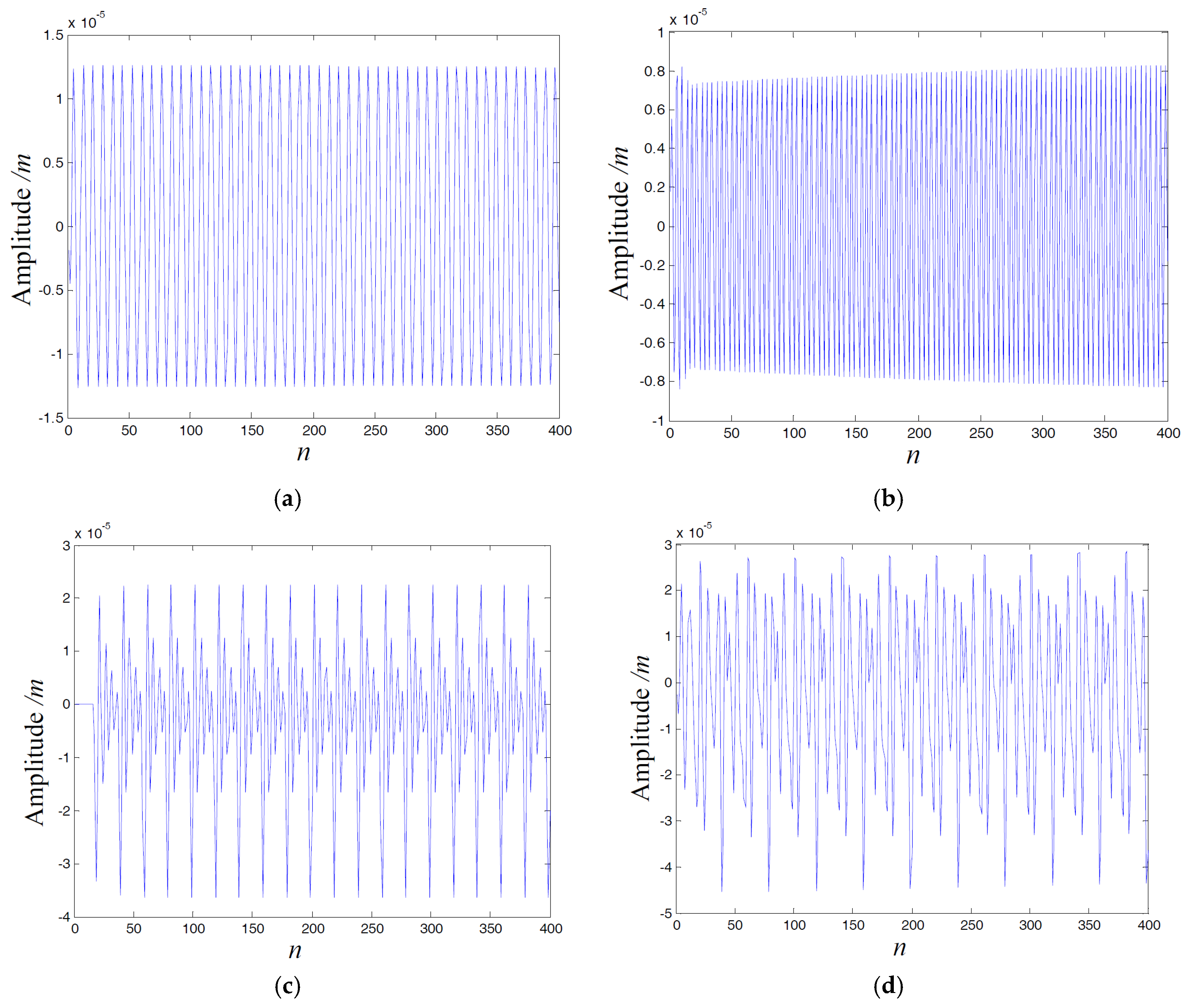
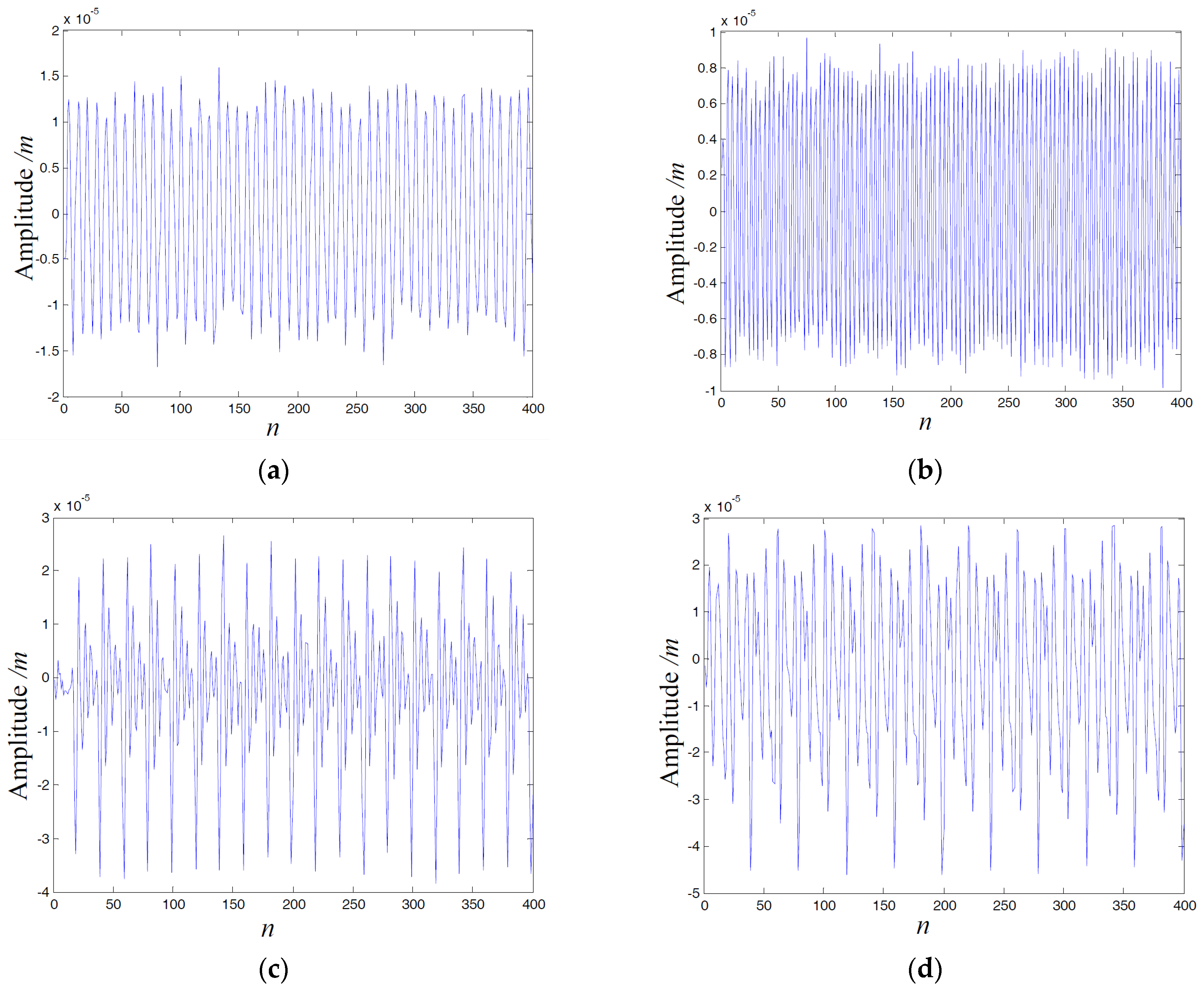
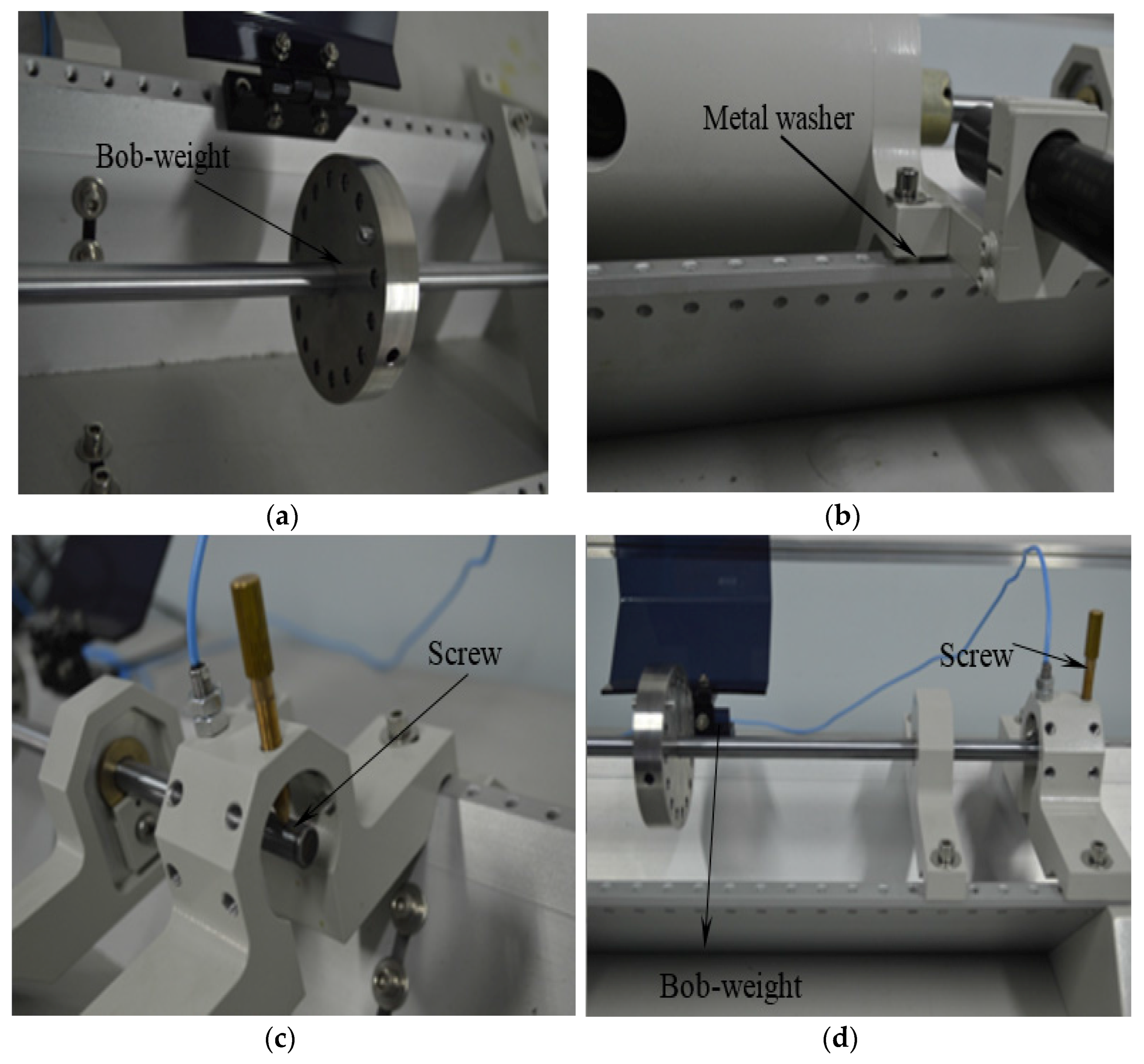
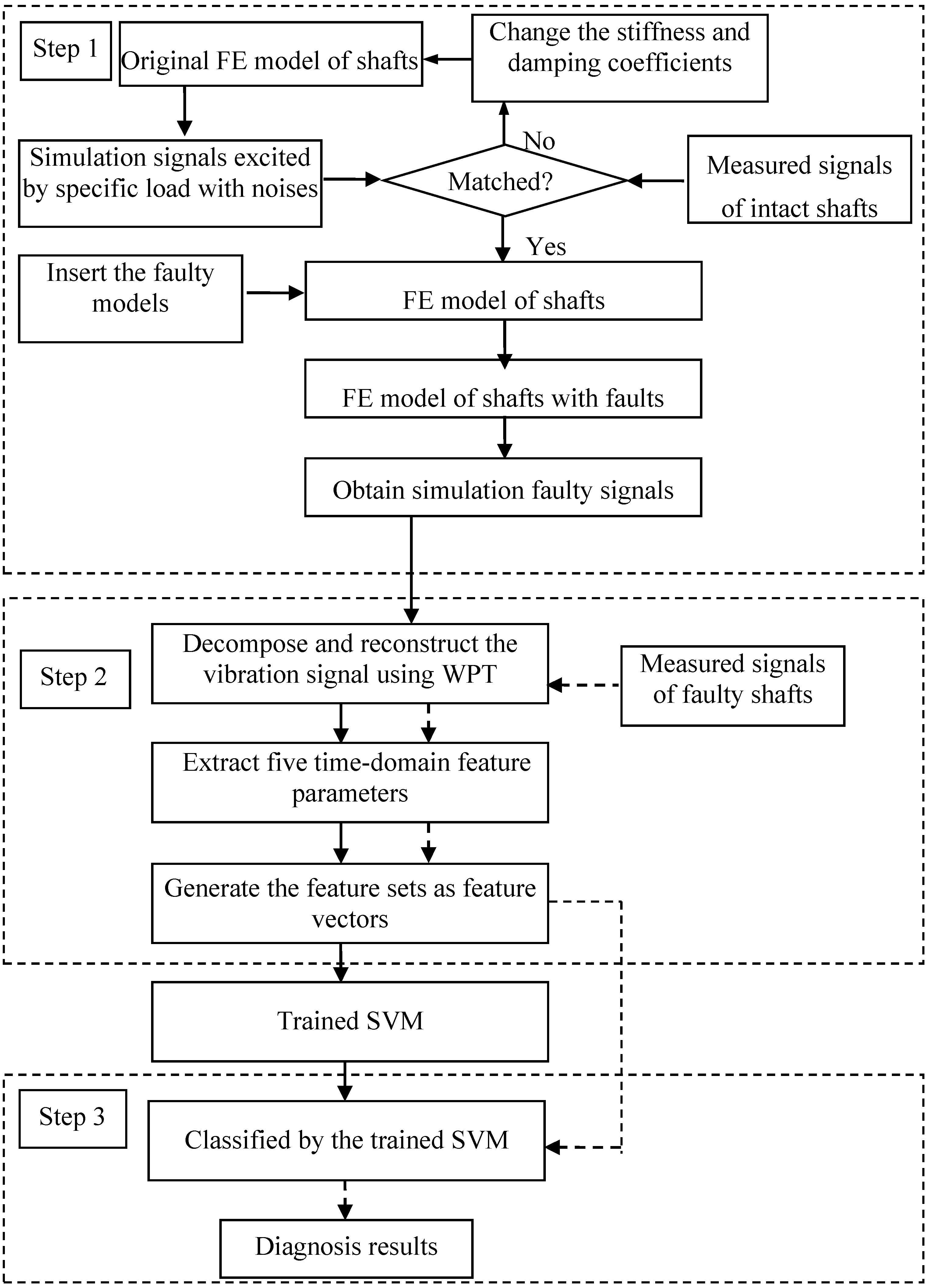
Intelligent diagnosis methods play a key role to prevent and detect faults in mechanical systems, except for the lack of faulty training samples. Motivated by molecular dynamics simulation-based personalized medicine, we develop the concept of the numerical simulation-based personalized diagnosis methodology and, more specifically, a personalized fault diagnosis method using FEM, WPT and SVM to detect faults in a shaft. Numerical and experimental investigations are performed, and the fault diagnosis of the shafts is given. In the simulation, the classification accuracy rates of unbalance, misalignment, rub-impact and the combination of rub-impact and unbalance are 93%, 95%, 89% and 91%, respectively. However, in the experimental investigations, this decreased to 82%, 87%, 73% and 79%. The results verified that the proposed method has the ability to distinguish the fault types. The numerical simulation-based personalized diagnosis methodology has many advantages, such as the activation of intelligent diagnosis methods by providing the complete faulty samples; the resolution of diagnosis reliability for a single machine stems from assembly variation with dynamic behaviors, influences from the operation environment, etc.

However, through the presented methodology, which is more likely to be expanded into more complex mechanical systems, such as gears, bearings, transmission systems, etc., the development of a standard FE model updating technique is the most important to obtain the agreeable numerical simulation faulty samples under different work conditions for the same type of mechanical systems. Furthermore, the computational cost is small for the present one-dimensional (1D) FE model employed. For complex mechanical systems, the calculation process is time consuming, but the proposed methodology only requires pre-computing the training samples, which serve as the inputs into the intelligent diagnostic models, such as SVM, GAs, NNs, etc.

References

1. Li, R.; Seçkiner, S.U.; He, D.; Bechhoefer, E.; Menon, P. Gear Fault Location Detection for split torque gearbox using AE sensors. IEEE Trans. Syst. Man Cybern. Part C 2012, 42, 1308–1317. [Google Scholar] [CrossRef]
2. Meng, L.; Xiang, J.; Wang, Y.; Jiang, Y.; Gao, H. A hybrid fault diagnosis method using morphological filter-translation invariant wavelet and improved ensemble empirical mode decomposition. Mech. Syst. Signal Process. 2015, 50, 101–115. [Google Scholar] [CrossRef]
3. Lei, Y.; Lin, J.; He, Z.; Zuo, M.J. A review on empirical mode decomposition in fault diagnosis of rotating machinery. Mech. Syst. Signal Process. 2013, 35, 108–126. [Google Scholar] [CrossRef]
4. Meng, L.; Xiang, J.; Zhong, Y.; Song, W. Fault diagnosis of rolling bearing based on second generation wavelet denoising and morphological filter. J. Mech. Sci. Technol. 2015, 29, 3121–3129. [Google Scholar] [CrossRef]
5. Jiang, B.Z.; Xiang, J.W.; Wang, Y.X. Rolling bearing fault diagnosis approach using probabilistic principal component analysis denoising and cyclic bispectrum. J. Vib. Control 2016, 22, 2420–2433. [Google Scholar] [CrossRef]
6. Xiang, J.W.; Zhong, Y.T.; Gao, H.F. Rolling element bearing fault detection using PPCA and spectral kurtosis. Measurement 2015, 75, 180–191. [Google Scholar] [CrossRef]
7. Xiang, J.; Lei, Y.; Wang, Y.; He, Y.; Zheng, C.; Gao, H. Structural dynamical monitoring and fault diagnosis. Shock Vib. 2015. [Google Scholar] [CrossRef]
8. Yang, Z.B.; Chen, X.F.; Xie, Y.; Zhang, X.W. The hybrid multivariate analysis method for damage detection. Struct. Control Health Monit. 2016, 23, 123–143. [Google Scholar] [CrossRef]
9. Yang, Z.B.; Chen, X.F.; Xie, Y.; Miao, H.H.; Gao, J.J.; Qi, K.Z. Hybrid two-step method of damage detection for plate-like structures. Struct. Control Health Monit. 2016, 23, 267–285. [Google Scholar] [CrossRef]
10. Zhang, X.; Wang, C.; Gao, R.X.; Yan, R.; Chen, X.; Wang, S. A novel hybrid error criterion-based active control method for on-line milling vibration suppression with piezoelectric actuators and sensors. Sensors 2016. [Google Scholar] [CrossRef] [PubMed]
11. He, D.; Li, R.; Zhu, J.; Zade, M. Data mining based full ceramic bearing fault diagnostic system using AE sensors. IEEE T. Neural Netw. 2011, 22, 2022–2203. [Google Scholar] [CrossRef] [PubMed]
12. He, D.; Li, R.Y.; Zhu, J.D. Plastic bearing fault diagnosis based on a two-step data mining approach. IEEE Trans. Ind. Electron. 2013, 60, 3429–3440. [Google Scholar] [CrossRef]
13. Qu, Y.Z.; He, D.; Yoon, J. Gearbox tooth cut fault diagnostics using acoustic emission and vibration sensors—A comparative study. Sensors 2014, 14, 1372–1393. [Google Scholar] [CrossRef] [PubMed]
14. Yoon, J.; He, D. Planetary gearbox fault diagnostic method using acoustic emission sensors. IET Sci. Meas. Technol. 2015, 9, 936–944. [Google Scholar] [CrossRef]
15. Mohammed, A.A.; Neilson, R.D. Crack detection in a rotating shaft using artificial neural networks and PSD characterization. Meccanica 2014, 49, 255–266. [Google Scholar] [CrossRef]
16. Torkaman, H.; Moradi, R.; Hajihosseinlu, A. A comprehensive power loss evaluation for switched reluctance motor in presence of rotor asymmetry rotation: Theory, numerical analysis and experiments. Energy Convers. Manag. 2014, 77, 773–783. [Google Scholar] [CrossRef]
17. Bregon, A.; Alonso-González, C.J.; Pulido, B. Integration of simulation and state observers for online fault detection of nonlinear continuous systems. IEEE Trans. Syst. Man Cybern. 2014, 44, 1553–1568. [Google Scholar] [CrossRef]
18. Gong, R.Z.; Wang, H.J.; Liu, Q.Z.; Shu, L.F.; Li, F.C. Numerical simulation and rotor dynamic stability analysis on a large hydraulic turbine. Comput. Fluids 2013, 88, 11–18. [Google Scholar] [CrossRef]
19. Xiang, J.W.; Jiang, Z.S.; Chen, X.F. A class of wavelet-based Rayleigh-Euler beam element for analyzing rotating shafts. Shock Vib. 2011, 18, 447–458. [Google Scholar] [CrossRef]
20. Xiang, J.W.; Long, J.Q.; Jiang, Z.S. A numerical study using Hermitian cubic spline wavelets for the analysis of shafts. Proc. Inst. Mech. Eng. Part C 2010, 224, 1843–1851. [Google Scholar] [CrossRef]
21. Tannous, M.; Cartraud, P.; Torkhani, M.; Dureisseix, D. Assessment of 3D modeling for rotor-stator contact simulations. J. Sound Vib. 2015, 353, 327–343. [Google Scholar] [CrossRef]
22. Baccarini, L.M.R.; Caminhas, W.M. Fault induction dynamic model, suitable for computer simulation: Simulation results and experimental validation. Mech. Syst. Signal Process. 2010, 24, 300–311. [Google Scholar] [CrossRef]
23. Chen, F.F.; Tang, B.P.; Song, T. Multi-fault diagnosis study on roller bearing based on multi-kernel support vector machine with chaotic particle swarm optimization. Measurement 2014, 47, 576–590. [Google Scholar] [CrossRef]
24. Liu, W.Y.; Han, J.G.; Lu, X.N. A new gear fault feature extraction method based on hybrid time–frequency analysis. Neural Comput. Appl. 2014, 25, 387–392. [Google Scholar] [CrossRef]
25. Li, N.; Zhou, R.; Hu, Q.; Liu, X. Mechanical fault diagnosis based on redundant second generation wavelet packet transform, neighborhood rough set and support vector machine. Mech. Syst. Signal Process. 2012, 28, 608–621. [Google Scholar] [CrossRef]
26. Xiang, J.; Matsumoto, T.; Wang, Y.; Jiang, Z. Detect damages in conical shells using curvature mode shape and wavelet finite element method. Int. J. Mech. Sci. 2013, 66, 83–93. [Google Scholar] [CrossRef]
27. Diego, R.I.; Barros, J. Global methods for time-frequency analysis of harmonic distortion in power systems using the wavelet packet transform. Electr. Power Syst. Res. 2009, 79, 1226–1239. [Google Scholar] [CrossRef]
28. Pan, Y.; Chen, J.; Guo, L. Robust bearing performance degradation assessment method based on improved wavelet packet-support vector data description. Mech. Syst. Signal Process. 2009, 23, 669–681. [Google Scholar] [CrossRef]
29. Vong, C.M.; Wong, P.K. Engine ignition signal diagnosis with wavelet packet transform and multi-class least squares support vector machines. Expert Syst. Appl. 2011, 38, 8563–8570. [Google Scholar] [CrossRef]
30. Liu, Z.; Cao, H.; Chen, X. Multi-fault classification based on wavelet SVM with PSO algorithm to analyze vibration signals from rolling element bearings. Neurocomputing 2013, 99, 399–410. [Google Scholar] [CrossRef]
31. Perkel, J.M. Life science technologies: Molecular diagnostics: Personalizing personalized medicine. Science 2009. [Google Scholar] [CrossRef]
32. Ledford, H. Personalized medicine takes hit. Nature 2016, 536, 382. [Google Scholar] [CrossRef] [PubMed]
33. Haines, J.L. Complement factor H variant increases the risk of age-related macular degeneration. Science 2005, 308, 419–421. [Google Scholar] [CrossRef] [PubMed]
34. Lei, Y.G.; Zuo, M.J.; He, Z.J. A multidimensional hybrid intelligent method for gear fault diagnosis. Expert Syst. Appl. 2010, 37, 1419–1430. [Google Scholar] [CrossRef]
35. Friswell, M.I.; Mottershead, J.E. Finite Element Model Updating in Structural Dynamics; Kluwer Academic Publishers: Amsterdam, The Netherlands, 1995. [Google Scholar]
36. Xiang, J.W.; Liang, M.; He, Y.M. Experimental investigation of frequency-based multi-damagedetection for beams using support vector regression. Eng. Fract. Mech. 2014, 131, 257–268. [Google Scholar] [CrossRef]
37. Kheir, N.A.; Holmes, W.M. Modeling and credibility of random ensembles. Simulation 1982, 38, 93–103. [Google Scholar] [CrossRef]
38. Jalan, A.K.; Mohanty, A.R. Model based fault diagnosis of a rotor–bearing system for misalignment and unbalance under steady-state condition. J. Sound Vib. 2009, 327, 604–622. [Google Scholar] [CrossRef]
39. Cao, H.R.; Niu, L.K.; He, Z.J. Method for vibration response simulation and sensor placement optimization of a machine tool spindle system with a bearing defect. Sensors 2012, 12, 8732–8754. [Google Scholar] [CrossRef] [PubMed]
40. Franc, V.; Hlavác, V. Statistical Pattern Recognition Toolbox for Matlab; Center for Machine Perception, Czech Technical University: Prague, Czech Republic, 2004. [Google Scholar]
41. Li, P.F.; Jiang, Y.Y.; Xiang, J.W. Experimental investigation for fault diagnosis based on a hybrid approach using wavelet packet and support vector classification. Sci. World J. 2014. [Google Scholar] [CrossRef] [PubMed]
Figure 1. The fundamental procedure of the personalized diagnosis methodology.
Applsci 06 00414 g001
Figure 2. The typical binary wavelet packet transform (WPT) decomposition structure (three layers).
Applsci 06 00414 g002
Figure 3. The flowchart of the proposed fault diagnosis method. Solid and dotted arrows mean the training and testing paths to realize the method.
Applsci 06 00414 g003
Figure 4. The finite element model of the shaft. (a) The geometry of the shaft, note: L1 = 0.1 m, L2 = 0.1 m, L3 = 0.25 m, L4 = 0.5 m, d1 = 0.01 m, d2 = 0.078 m, h1 = 0.01 m, ∆L = 0.002 m; (b) the linear bearing model.
Applsci 06 00414 g004
Figure 5. The simulation signals with different kinds of faults. (a) Unbalance; (b) misalignment; (c) rub-impact; (d) the combination of rub-impact and unbalance.
Applsci 06 00414 g005
Figure 6. The exciting force in each direction of the rub-impact: (a) the exciting force in x-direction; (b) the exciting force in y-direction.
Applsci 06 00414 g006
Figure 7. Simulation signals by adding noises (Signal-to-noise ratio (SNR) = 97). (a) Unbalance; (b) misalignment; (c) rub-impact; (d) the combination of rub-impact and unbalance.
Applsci 06 00414 g007
Figure 8. Simulation signals after adding noises (SNR = 87). (a) Unbalance; (b) misalignment; (c) rub-impact; (d) the combination of rub-impact and unbalance.
Applsci 06 00414 g008
Figure 9. The experimental setup of a rotor-bearing system under normal load conditions.
Applsci 06 00414 g009
Figure 10. Four faults of a shaft in the experimental operation. (a) Unbalance; (b) misalignment; (c) rub-impact; (d) the combination of rub-impact and unbalance.
Applsci 06 00414 g010
Figure 11. The measured signals with different kinds of faults. (a) The measured signals with unbalance fault; (b) the measured signals with misalignment fault; (c) the measured signals with rub-impact fault; (d) the measured signals with the combination of rub-impact and unbalance fault.
Applsci 06 00414 g011