Automatic Taxonomic Classification of Fish Based on Their Acoustic Signals

Abstract

Fish as well as birds, mammals, insects and other animals are capable of emitting sounds for diverse purposes, which can be recorded through microphone sensors. Although fish vocalizations have been known for a long time, they have been poorly studied and applied in their taxonomic classification. This work presents a novel approach for automatic remote acoustic identification of fish through their acoustic signals by applying pattern recognition techniques. The sound signals are preprocessed and automatically segmented to extract each call from the background noise. Then, the calls are parameterized using Linear and Mel Frequency Cepstral Coefficients (LFCC and MFCC), Shannon Entropy (SE) and Syllable Length (SL), yielding useful information for the classification phase. In our experiments, 102 different fish species have been successfully identified with three widely used machine learning algorithms: K-Nearest Neighbors (KNN), Random Forest (RF) and Support Vector Machine (SVM). Experimental results show an average classification accuracy of 95.24%, 93.56% and 95.58%, respectively.

1. Introduction

Researchers have found that more than 800 fish species are able to produce sounds for diverse purposes [1,2]. Most of the sounds are emitted at low frequencies [3], usually below 1000 Hz. However, some pulses can reach 8 kHz [4,5] or present more complex characteristics [6]. In addition, these emissions are typically broadband short-duration signals (see Figure 1). Fish generate sounds through several mechanisms, which depend on the species and a variety of circumstances, such as courtship, threats or defending territory [7]. Hence, most fish make species-specific acoustic signals that can be gathered using passive acoustic sensors (hydrophones).

Passive acoustic surveys are widely used to monitor presence/absence of marine fauna, tracking their movement or estimating seasonal distribution, especially in the study of marine mammals [8,9]. These recordings typically include noise from the natural environment and anthropogenic sources [10], which have to be suppressed to focus on biological signals. Anthropogenic noise has become one of the greatest sources of background noise in oceans, which is produced by human activity: commercial shipping, oil extraction, fishing, etc. Moreover, passive acoustic sensors offer advantages over visual monitoring systems in waters with poor visibility and with adverse weather conditions [11].

Several techniques have been applied to characterize acoustic vocalizations in wildlife animals for automatic detection and classification. Exhaustive studies have been conducted in birds [12], amphibians [13], insects [14] and bats [15] with varying degrees of success. As for marine fauna, some works can be found in the literature concerning the acoustic identification of whales and dolphins. Gillespie et al. [16] developed a classification system to work with fragmented whistle detections of four odoncetes, achieving a 94% classification rate. However, when the number of species was increased, system accuracy dropped heavily. In [17], four types of dolphin calls were identified using a Fourier Descriptor (FD) to characterize the whistlers shape. Then, K-Nearest Neighbors (KNN) and Support Vector Machine (SVM) were employed as classifiers. In the end, statistical significant results were not obtained due to the small corpus.

Different fish species are mainly recognized by sonar images based on shape and geometric features or by computer vision technologies. For instance, in [18], three species of fish were identified using acoustic echo sounder surveys and applying the SVM classifier. Sonar echoes were parametrized by a set of features: morphology, acoustical energy, bathymetry and school–shore distance. In this work, a classification rate of 89.95% was achieved. As for the visual techniques, in [19], ten species of fish were successfully classified by a Balance-Guaranteed Optimized Tree (BGOT) using a combination of features such as color, shape and texture image properties with 95% accuracy.

Nevertheless, a robust intelligent system that identifies fish species by their acoustic signals has still not been found. Most previous efforts have limited their research to the spectro-temporal characterization of sound production, and the authors are only aware of a few studies [20,21] that have utilized the unique acoustic properties of fish for automatic identification. In [20], Kottege et al. analyzed the sound clicks of the Tilapia mariae fish by applying logistic regression and parameterizing the signal with a vector of six spectro-temporal features (STF). However, the syllables for training purposes were manually selected. Meanwhile, Ruiz et al. [21] presented a method that automatically identifies acoustic emissions of two sciaenid fish by threshold decision. This approach used pitch strength, drumming frequency and short/long term partial loudness as features producing satisfactory results, but the proposed system was hardly scalable.

On the other hand, fish vocalizations can be monitored through autonomous hydrophone arrays or vector sensors [22]. The vector hydrophone measures the direction of sound vibration and sound intensity, so it presents advantages in the detection of underwater acoustic targets emitting low and ultra-low frequency signals [23] such as fish sounds. These technologies are relatively inexpensive and possess remote monitoring capabilities for long-term data acquisition. Thus, they have become a valuable tool for biological studies, ecological conservation and fish population estimation.

The aim of this work is to design and implement a robust and novel automatic system for the identification of fish from its acoustic signals. Therefore, it could be used to map species and detect changes in fauna composition. For this purpose, four types of features have been extracted for each call, which have been fused into a single vector. To the best of our knowledge, this research is the first to fuse frequency (Mel and Linear Frequency Cepstral Coefficients) and temporal (Shannon entropy and call duration) fish acoustic features. The main novelty of this work comes from the fact that these features are combined to achieve a robust representation of the sound. Moreover, the results of three widely used pattern matching techniques have been compared to test the approach: KNN [24], Random Forest (RF) [25] and SVM [26]. This system has been validated on a dataset composed of 102 marine animals from two public sound collections that were previously labeled by experts.

The remainder of this paper is organized as follows: Section 2 describes the proposed system and introduces the acoustic data. The classification methods used (SVM, RF and KNN) are described in Section 3, particularized for acoustic recognition. Then, Section 4 contains the experimental methodology. Section 5 provides details and discusses the results obtained. Finally, in Section 6, the conclusions of this work are shown.

2. Proposed System

The proposed system is based on the following phases: first, samples of fish acoustic signals are gathered using underwater sound sensors and stored in audio files. These recordings are preprocessed to adapt the input signal. Secondly, the acoustic signal is automatically segmented in syllables and labeled by species. The features are extracted from each syllable and grouped into a single vector. Afterwards, they are used to train the classification algorithm. 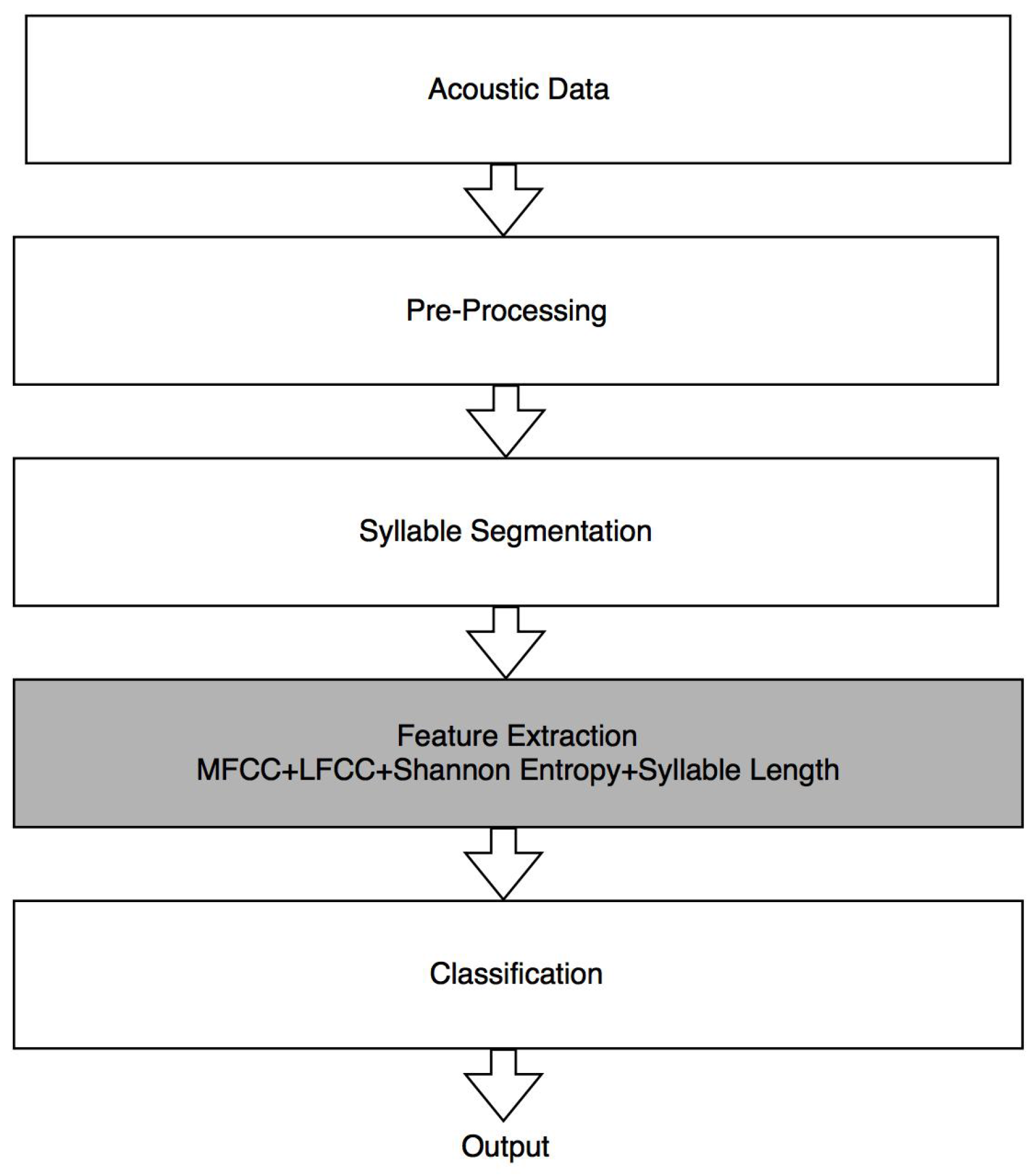Figure 2 illustrates the proposed system.

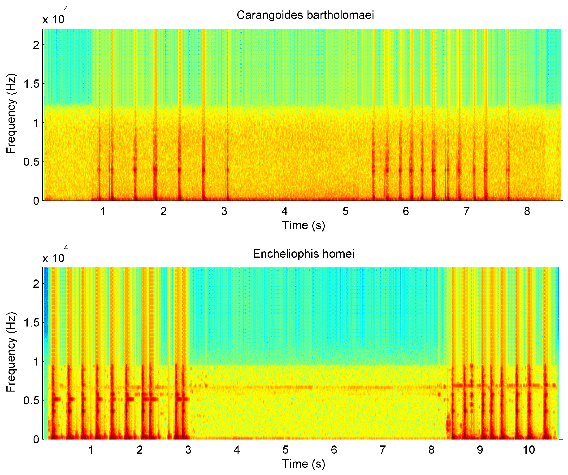
2.1. Acoustic Data

A sound dataset has been constructed using two Internet sound collections. The main source of audio recordings has been taken from FishBase [27], which is a database developed by the WorldFish Center (Penang, Malaysia) in collaboration with the Food and Agriculture Organization of the United Nations (FAO). FishBase contains information of 33,200 species and 258 sound recordings with an average duration of 14 seconds, belonging to 90 different classes of fish taken with ambient noise from hydrophone sensors. Most of these recordings come from the previous work of [28], where various sounds were obtained from fish tanks avoiding some sources of anthropogenic noise. However, the tanks added other noise sources such as the fish tank pump and bubbling water. Furthermore, 55.91% of the sounds were obtained under duress (manual or electrically stimulated) or artificial conditions, and the rest of the sounds were spontaneous or gathered under natural conditions. The second database, DOSITS (Discovery of Sound In The Sea) [29], is a project of the University of Rhode Island to divulge information about underwater sound research. DOSITS contains 23 audio files of 21 fish species, but it presents nine classes in common with FishBase. In addition, audio files have been sampled at 44.1 kHz in both collections. Therefore, the dataset is finally composed of 102 different fish species with approximately 18 samples for each class.

2.2. Preprocessing

Most of the sounds emitted by fish are at low frequencies, typically below 1000 Hz [3], but some of them can produce sounds with frequencies above 8 kHz [5]. Therefore, the input signal is low-pass filtered at 10 kHz to suppress the high frequency background noise.

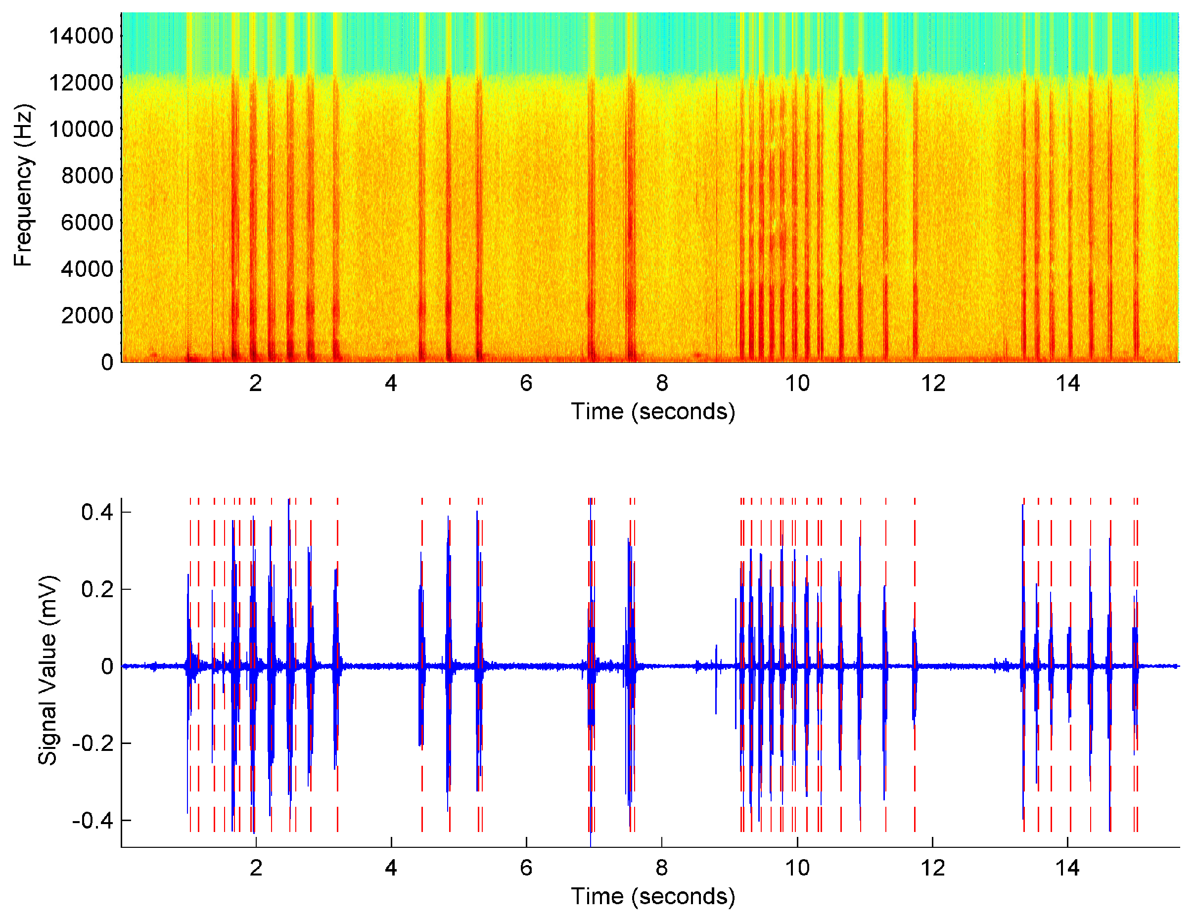
2.3. Segmentation

In the segmentation phase, audio signals are automatically split into syllables isolating each acoustic sound. This procedure is performed applying the method developed by Härmä in [30]. It carries out the Short Time Fourier Transform (STFT) to obtain the spectrogram representation of the signal denoted as $M(f,t)$, where f is the frequency index and t represents the time index. Then, the algorithm proceeds as follows:

• Find the highest amplitude peak such as $|M(f_n,t_n)|\ge |M(f,t)|\forall (f,t)$ and set the position of the nth syllable in $t_n$. The amplitude of this point is calculated as Equation (1):

  $$Y_n\left(0\right)=20{\log }_{10}\left(\right|M(f_n,t_n)\left|\right).$$

  (1)
• Trace the adjacent peaks between $t>t_n$ and $t<t_n$ until $Y_n(t-t_n)<Y_n\left(0\right)-\mathsf{\beta }dB$, where $\mathsf{\beta }$ is the stopping criterion. Thus, the starting and ending times of the nth syllable are defined as $t_n-t_s$ and $t_n+t_e$.
• This trajectory is saved as the nth syllable and deleted from matrix (2):

  $$M(f_n,t_n-t_s,\cdots ,t_n+t_e)=0.$$

  (2)
• Repeat the process from step 1 until the end of the spectrogram.

In this approach, STFT is computed using a Hamming window of 512 samples with an overlap of 35%, which has been set experimentally. Furthermore, a stopping criterion of $\mathsf{\beta }=20\mathrm{dB}$ has been selected. The algorithm is applied in all 102 classes used in this paper. Figure 3 shows the results of the process where the red dashed lines indicate the central points of the syllables detected by the algorithm in the signal.

3. Feature Extraction

After performing the segmentation, temporal and frequency domain characteristics have been computed for each syllable to yield useful information for the taxonomic classification.

In this paper, the syllables have been spectrally characterized by LFCCs and MFCCs to hold information of lower and higher frequency regions of the signal [31]. These coefficients are similarly calculated based on short-time analysis, using a Hamming window of 25 milliseconds with an overlap of 45% for both features. In addition, MFCC required a frequency scale transformation from Hertz to Mel scale (3) performed by a set of 26 triangular band-pass filters:

$$m=2595{\log }_{10}\left(\frac{f}{700}+1\right).$$

(3)

The final MFCC features were obtained from the Discrete Cosine Transform (DCT) of the log-magnitude output of each triangular filter, $Y_i$. They are computed following Equation (4), where N is the number of cepstral coefficients and M denotes the number of triangular filters:

$${\mathrm{MFCC}}_j=\sum _{i=1}^M\left(\log \right|Y_i|\cos [j(i-\frac{1}{2})]\mathsf{\pi }/M),0\le j\le N-1.$$

(4)

LFCCs are directly calculated from the log-magnitude Discrete Fourier Transform (DFT) as is indicated in Equation (5), where K denotes the number of DFT magnitude coefficients ($|X_i|$). The number of coefficients have been selected by experimentation in order to seek the best accuracy. Finally, $N=18$ coefficients have been taken for both MFCCs and LFCCs, in all experiments:

$${\mathrm{LFCC}}_j=\sum _{i=0}^{K-1}\left(\log \right|X_i|\cos [\frac{ji\mathsf{\pi }}{K}]),1\le j\le N.$$

(5)

Furthermore, temporal discriminant attributes have also been extracted from each segment, Shannon Entropy (SE) [32] and Syllable Length (SL), to obtain a robust representation of the fish acoustic signal. Finally, the coefficients are grouped in vectors as shown in Label (6), where each vector has 38 coefficients (18 MFCCs + 18 LFCCs + 1 SE + 1 SL) per row. These vectors are used to feed the classification algorithms in the next stage. This information of higher and lower frequency regions and time variable features have been combined to achieve a complete characterization of the sound:

$$\mathrm{Parameters}=\left[\mathrm{MFCC}\mathrm{LFCC}\mathrm{SE}\mathrm{SL}\right].$$

(6)

4. Classification Methods

In the classification stage, three machine learning algorithms, KNN, RF and SVM, have been employed to conduct a comparative study of task performance. The next subsections show the implementation details of the algorithms used in this work.

4.1. K-Nearest Neighbor

KNN is a machine learning algorithm that predicts the classification of new data based on the closest training samples in the feature space. The algorithm decides which class is similar by picking the K nearest data point distances to the observation. Then, it simply uses the majority of nearest neighbors to determine the class prediction. In this approach, the number of nearest neighbors was established in $K=\sqrt{n}$ using Euclidean distance, where n is the number of features.

4.2. Random Forest

The algorithm bundles randomly generated decision trees (DT) in which each tree tries to classify the data interdependently using a bootstrapped random subset of the training samples. In essence, trees are trained as follows:

• A set of N syllables are randomly extracted with replacement from the training data.
• Let M be the number of coefficients in a syllable. At each node m, random features are selected such as $m<<M$ seeking the best split over these m variables.

Finally, RF makes the prediction taking the most popular voted class from all tree predictors in the forest, as is shown in (7). In this paper, $K=200$ trees have been utilized to classify the fish sounds, fixing the number of predictor variables to $m=\sqrt{M}$.

$$\mathrm{Prediction}={\mathrm{argmax}}_c(\sum _{i=1}^K{Y}_i=c), \mathrm{where} Y_i \mathrm{is} \mathrm{the} i\mathrm{th} \mathrm{tree} \mathrm{vote}.$$

(7)

4.3. Support Vector Machine

SVM is a supervised machine learning algorithm that maps input data as points of a higher dimensional space, splitting them in non-overlapping hyperplanes. The decision boundary is decided by the calculation of the optimal partition that separates the training data into two classes. Besides this, the technique is able to work with nonlinear separable data through kernel functions, where the classes are divided into a higher dimensional space. In this research, the algorithm has been implemented based on the libsvm library [33] with a Gaussian kernel function K that has been selected after trials with different kernels. For the experiments, $K(x,x^{\prime })=\exp (-c\parallel x-x^{\prime }{\parallel }^2)$ has been used with $c=0.45$. Moreover, SVM only recognizes two classes, so the strategy “one-versus-one” [34] has been selected to perform the multiclass classification. Therefore, it has generated $N(N-1)/2$ SVM binary classifiers, where N represents the number of fish species.

5. Experimental Procedure

In order to evaluate the effectiveness of the proposed system, the features have been incrementally grouped in the experiments to analyze the contribution of each attribute to the final approach. At the same time, the acoustic features have been combined with the classification algorithms to seek the best performance. To ensure independence between the training and testing sets in each simulation (at least 100 simulations by experiments), the syllables obtained automatically from the segmentation of each sound have been randomly shuffled and split 50/50 into two datasets, one for training and another for testing (k-fold cross-validation with k = 2) to achieve significant results. Furthermore, accuracy has been calculated following Equation (8) for each class and averaging the results. F-Measure value [35] has also been calculated as $2\ast \left(\right(P\ast R)/(P+R\left)\right)$, where P (precision) is the number of correct positive results divided by the number of all positive results, and R (recall) is the number of correct positive results divided by the number of positive results:

$$\mathrm{Accuracy}(\%)=\frac{\mathrm{Syllables} \mathrm{Correctly} \mathrm{Identified}\left(N_c\right)}{\mathrm{Total} \mathrm{Number} \mathrm{of} \mathrm{Syllables}\left(N_s\right)}\times 100.$$

(8)

Results and Discussions

The experiments consisted of two phases. The first phase performed an evaluation of different algorithms and features in order to find the best model capable of recognizing fish calls. For that reason, 50% of the feature vector samples have been taken for training purposes and the rest for testing. In the second stage, the training samples have been reduced to 5% in order to verify the robustness of the methodology.

Table 1. Classification results.

Dataset	Features	Classification	Training time (s)	Test time (s)	Accuracy Median % ± Std.
Fish dataset (102 species)	MFCC ${}^1$	KNN ${}^1$	0.04	0.01	91.94% ± 15.27%
		RF ${}^1$	0.76	0.01	90.34% ± 15.01%
		SVM ${}^1$	0.28	0.09	91.20% ± 18.25%
	LFCC ${}^1$	KNN	0.04	0.01	89.05% ± 16.04
		RF	0.76	0.01	87.41% ± 16.46%
		SVM	0.25	0.09	81.60% ± 28.14%
	MFCC + LFCC	KNN	0.05	0.02	94.27% ± 11.10%
		RF	1.29	0.02	93.63% ± 10.59%
		SVM	0.31	0.10	94.72% ± 12.13%
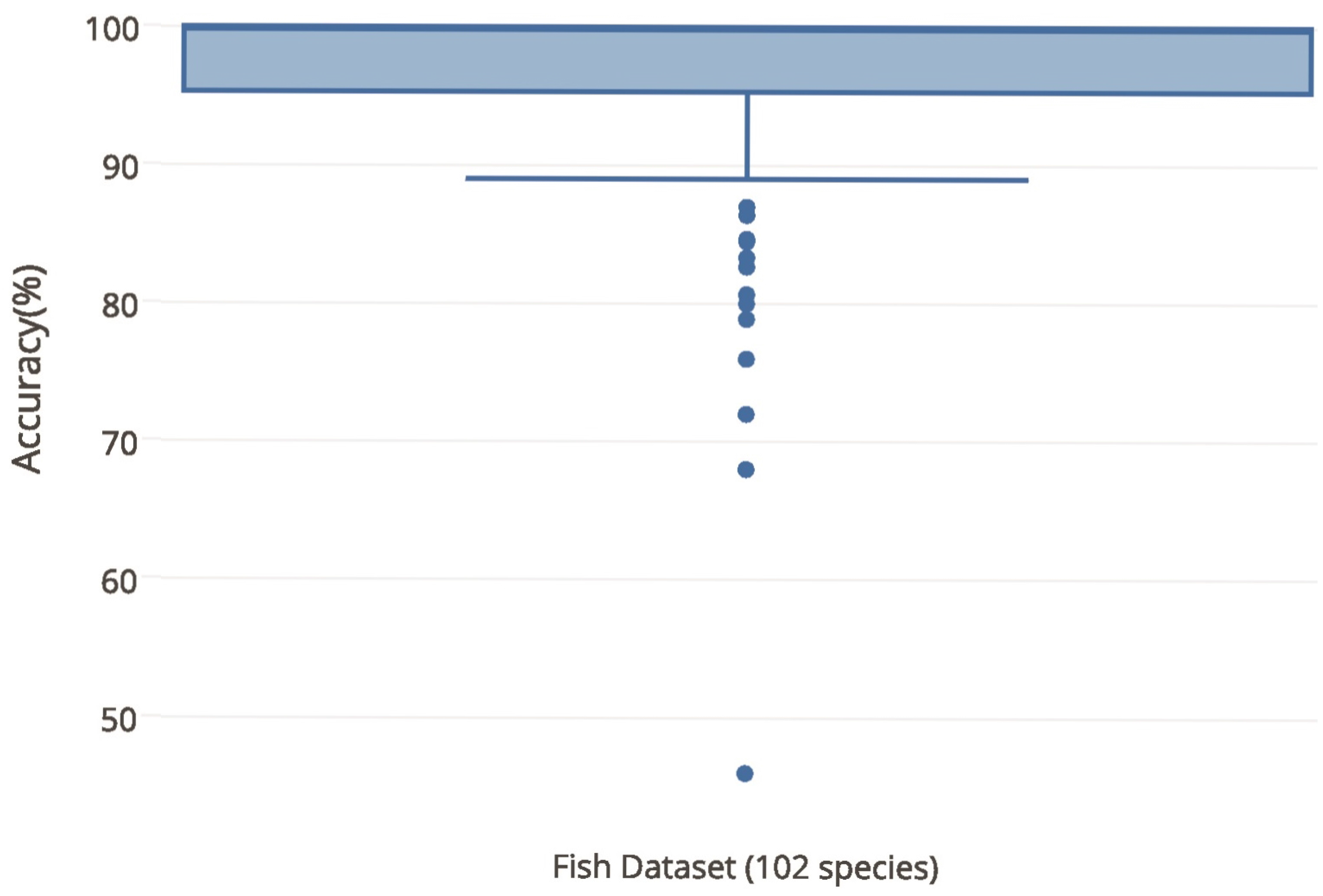
	MFCC + LFCC + SE ${}^1$ + SL ${}^1$	KNN	0.05	0.02	95.24% ± 8.59%
		RF	1.14	0.01	93.56% ± 11.42%
		SVM	0.34	0.10	95.58% ± 8.59%

${}^1$ MFCC: Mel Frequency Cepstral Coefficients; KNN: K-Nearest Neighbors; RF: Random Forest; SVM: Support Vector Machine; LFCC: Linear Frequency Cepstral Coefficients; SE: Shannon Entropy; SL: Syllable Length.

shows how the proposed combination of features reinforces the learning procedure as a consequence of fusing the temporal and frequency information, regardless of the algorithm used. MFCCs clearly outperform LFCCs when used individually because fish acoustic signals are basically generated in low frequencies and MFCCs coefficients emphasize that region of the spectrum. Meanwhile, LFCCs represent higher frequencies better so they perform poorly in all experiments. In fact, three species could not be identified at all: Haemulon flavolineatum, Merluccius bilinearis and Diplectrum formosum. To parametrize lower as well as higher frequencies, both features were fused (MFCC + LFCC). The experiments verified that the fusion of information increases the performance of the system enhancing the recognition rate. Finally, the temporal information has been added, SE and SL, achieving an evident improvement in accuracy. It simplifies the work of the classifier due to significant temporal differences among the fish calls. Therefore, it confirms that the proposed system is effective for identifying and classifying fish acoustic signals with a high success rate.

As expected, KNN requires the lowest training times due to its simplicity. Even so, KNN outperforms other algorithms in the first two scenarios, applying MFCCs and LFCCs independently. In this case, SVM and RF are not able to extract discriminant information to separate the classes properly. After grouping the features, SVM slightly surpasses KNN and overcomes RF. The reason lies in the fact that SVM with the Gaussian kernel performs better than KNN with nonlinear data. Furthermore, RF needs a larger set of training data to define a robust model. Finally, the SVM approach based on temporal-frequency characteristics achieves the best taxonomic classification rate of 95.58%. Hence, it was selected for the rest of the experiments.

Figure 4 presents the average accuracy results for each class where the best approach was applied (MFCC-LFCC-SE-SL with SVM). It reveals poor classification rates in two classes that cannot be identified properly, and only six species obtained an accuracy lower than 80%. The lowest identification rate was 46% for Morone saxatilis, whose sounds are constantly mistaken with Pomadasys corvinaeformis and Conodon nobilis, due to similar frequency responses. The second lowest classification is for Trachinotus goodei with an accuracy of 68%. This recording presented high background noise and only four segmented syllables during the identification phase. However, 58 species reached 100% success, as a consequence of their distinct spectral characteristics.

The following experiment verified that this approach is able to deal with a low number of training samples that were progressively reduced from 50% to 5%. In

Table 2. Classifier performance by training set size.

Training Data (%)	Accuracy Median (%) ± Std.	Precision	Recall	F-Measure
5	81.77% ± 21.08%	0.8114	0.8168	0.8141
10	83.27% ± 19.17%	0.8385	0.8318	0.8351
20	88.15% ± 15.18%	0.8826	0.8807	0.8817
30	92.57% ± 13.92%	0.9191	0.9244	0.9218
40	94.99% ± 7.99%	0.9426	0.9490	0.9458
50	95.58% ± 8.59%	0.9535	0.9558	0.9546

, the evaluation shows that the system can operate reasonably well under these circumstances. Only when the number of samples drops to 10% does the system show clear signs of decline in effectiveness. At this level, most species are only represented by one or two samples, thus SVM has serious difficulties in finding an optimal separation boundary among classes. Nevertheless, this approach is able to maintain the results of classification above 80%. Hence, it confirms the robustness of the technique.

Finally, an experiment has been performed applying our best approach (data fusion + SVM) splitting the database into two subsets: sounds obtained under duress (manual or electrically stimulated) or artificial conditions (“unnatural sounds”) and sounds generated spontaneously or under natural conditions (“natural sounds”). Approximately 55.91% of the sounds are considered “unnatural” and the rest, 44.09%, as “natural”. Performance results are shown in

Table 3. Classifier performance by sound type.

Dataset	Accuracy Median (%) ± Std.	Precision	Recall	F-Measure
“Unnatural sounds”	95.21% ± 8.26%	0.9452	0.9520	0.9486
“Natural sounds”	98.17% ± 6.48%	0.9839	0.9817	0.9828

.

Regardless of the nature of the sound, the proposed system is able to perform an efficient classification. The results are better than in previous experiments due to the reduction of the complexity of the problem. Furthermore, the “natural sounds” dataset achieved a higher result than the “unnatural sounds” dataset as a consequence of reverberant sounds with high frequency harmonics that are produced under artificial conditions.

As mentioned previously, the number of studies concerning fish acoustic signals through intelligent systems is very limited. Therefore, a comparative study has been done with other state-of-the-art fish recognition techniques based on sonar images and morphological features.

Table 4. Comparison of the proposed system vs. state-of-the-art.

Reference	Database	Features	Classification	Accuracy
[21]	2 species	Drumming frequency, pitch, short and long term partial loudness	Threshold	80% and 90%
[18]	3 species	Morphology, spatial location, acoustic energy and bathymetry	SVM ${}^1$	89.55%
[36]	2 species	Morphology	SVM	78.59%
[19]	10 species	Color, texture and morphology	BGOT ${}^1$	91.70%
[37]	15 species	Euclidean network technique, quadratic network technique and triangulation technique	Bayesian	75.71%
This work	Fish dataset (102 species)	MFCC/LFCC/SE/SL ${}^1$	SVM	95.58% ± 8.59%

${}^1$ SVM: Support Vector Machine; BGOT: Balanced-Guaranteed Optimized Tree; MFCC: Mel Frequency Cepstral Coefficients; LFCC: Linear Frequency Cepstral Coefficients; SE: Shannon Entropy; SL: Syllable Length.

draws attention to the discriminating capabilities of acoustic fish signals regarding visual methods. The proposed system was able to recognize a larger dataset of fish species with a higher classification rate than other techniques.

6. Conclusions

Fish acoustic communication capabilities are well-known from literature; however, their species-specific characteristics have been little studied for automatic identification purposes. In this paper, we have introduced a novel automatic classification method of fish species based on their bioacoustic emissions, which allows the analysis of remote underwater data without human intervention. The acoustic signals have been parameterized through a combination of time-variable and frequency domain information, obtaining a complete representation of the signals. The results of this approach are promising with an average classification accuracy of 95.58% and a standard deviation of 8.59%. This shows that the proposed system achieves a better recognition rate than other methods based on computer vision techniques. Hence, these results suggest that this technique should be studied as an alternative method for estimation of fishery resources or to map species biodiversity. It has been verified over a dataset formed of 102 fish species with a relatively low number of samples. Unfortunately there are few public datasets of fish sounds to perform a broad study. In fact, the authors are not aware of other studies that have automatically and acoustically classified such a large number of fish species. Furthermore, the system has been tested in small training set scenarios, proving the robustness of the method. Even using only 5% of the samples for training, the system was able to achieve results above 80%.

In this research, it has also been found that MFCCs are more efficient for modeling these signals due to the sounds produced by fish mainly being emitted at low frequencies. However, adding information of high frequencies through LFCCs has significantly improved the performance on the test set. Finally, temporal information has been incorporated into the model, Shannon Entropy and Syllable Length, achieving a stronger taxonomic classification system due to the clear temporal differences among their acoustic signals. On the other hand, the system performance was quite similar for the different types of machine learning algorithms used, with differences below 2% in most cases, although SVM has been proven to be more effective in the bioacoustic recognition task because of the data showing nonlinear relationships.

However, further work should be done in order to reach a high quality solution. At least 800 fish species have been reported to produce bioacoustic sounds, so it is necessary to extend the corpus with additional species. Furthermore, in shallow water, low frequency signals present little range of propagation. Therefore, passive techniques should be combined with active acoustics and video methods to increase the scope of application. On the other hand, long-term acoustic surveys should be collected under natural conditions that would increase data quality and fine-tune the system for real world applications.

References

- Kaatz, I.M. Multiple sound-producing mechanisms in teleost fish and hypotheses regarding their behavioural significance. Bioacoustics 2002, 12, 230–233. [Google Scholar] [CrossRef]
- Rountree, R.A.; Gilmore, R.G.; Goudey, C.A.; Hawkins, A.D.; Luczkovich, J.J.; Mann, D.A. Listening to fish: applications of passive acoustics to fisheries science. Fisheries 2006, 31, 433–446. [Google Scholar] [CrossRef]
- Ladich, F. Sound production and acoustic communication. In The Senses of Fish; Springer: Berlin, Germany, 2004; pp. 210–230. [Google Scholar]
- Zelick, R.; Mann, D.A.; Popper, A.N. Acoustic communication in fish and frogs. In Comparative Hearing: Fish and Amphibians; Springer: Berlin, Germany, 1999; pp. 363–411. [Google Scholar]
- Tavolga, W.N.; Popper, A.N.; Fay, R.R. Hearing and Sound Communication in Fish; Springer Science & Business Media: Berlin, Germany, 2012. [Google Scholar]
- Vasconcelos, R.O.; Fonseca, P.J.; Amorim, M.C.P.; Ladich, F. Representation of complex vocalizations in the Lusitanian toadfish auditory system: Evidence of fine temporal, frequency and amplitude discrimination. Proc. Biol. Sci. 2011, 278, 826–834. [Google Scholar] [CrossRef] [PubMed]
- Kasumyan, A. Sounds and sound production in fish. J. Ichthyol. 2008, 48, 981–1030. [Google Scholar] [CrossRef]
- Morrissey, R.; Ward, J.; DiMarzio, N.; Jarvis, S.; Moretti, D. Passive acoustic detection and localization of sperm whales (Physeter macrocephalus) in the tongue of the ocean. Appl. Acoust. 2006, 67, 1091–1105. [Google Scholar] [CrossRef]
- Marques, T.A.; Thomas, L.; Ward, J.; DiMarzio, N.; Tyack, P.L. Estimating cetacean population density using fixed passive acoustic sensors: An example with Blainville’s beaked whales. J. Acoust. Soc. Am. 2009, 125, 1982–1994. [Google Scholar] [CrossRef] [PubMed]
- Hildebrand, J.A. Anthropogenic and natural sources of ambient noise in the ocean. Mar. Ecol. Prog. Ser. 2009, 395, 5–20. [Google Scholar] [CrossRef]
- Mellinger, D.K.; Stafford, K.M.; Moore, S.; Dziak, R.P.; Matsumoto, H. Fixed passive acoustic observation methods for cetaceans. Oceanography 2007, 20, 36. [Google Scholar] [CrossRef]
- Fagerlund, S. Bird species recognition using support vector machines. EURASIP J. Appl. Signal Process. 2007, 2007, 64. [Google Scholar] [CrossRef]
- Acevedo, M.A.; Corrada-Bravo, C.J.; Corrada-Bravo, H.; Villanueva-Rivera, L.J.; Aide, T.M. Automated classification of bird and amphibian calls using machine learning: A comparison of methods. Ecol. Inform. 2009, 4, 206–214. [Google Scholar] [CrossRef]
- Ganchev, T.; Potamitis, I.; Fakotakis, N. Acoustic monitoring of singing insects. In Proceedings of the IEEE International Conference on Acoustics, Speech and Signal Processing (ICASSP 2007), Honolulu, HI, USA, 15–20 April 2007.
- Henríquez, A.; Alonso, J.B.; Travieso, C.M.; Rodríguez-Herrera, B.; Bolaños, F.; Alpízar, P.; López-de Ipina, K.; Henríquez, P. An automatic acoustic bat identification system based on the audible spectrum. Expert Syst. Appl. 2014, 41, 5451–5465. [Google Scholar] [CrossRef]
- Gillespie, D.; Caillat, M.; Gordon, J.; White, P. Automatic detection and classification of odontocete whistles). J. Acoust. Soc. Am. 2013, 134, 2427–2437. [Google Scholar] [CrossRef] [PubMed]
- Esfahanian, M.; Zhuang, H.; Erdol, N. On contour-based classification of dolphin whistles by type. Appl. Acoust. 2014, 76, 274–279. [Google Scholar] [CrossRef]
- Bosch, P.; López, J.; Ramírez, H.; Robotham, H. Support vector machine under uncertainty: An application for hydroacoustic classification of fish-schools in Chile. Expert Syst. Appl. 2013, 40, 4029–4034. [Google Scholar] [CrossRef]
- Huang, P.X.; Boom, B.J.; Fisher, R.B. Underwater Live Fish Recognition Using a Balance-Guaranteed Optimized Tree. In Computer Vision—ACCV 2012; Springer: Berlin, Germany, 2012; pp. 422–433. [Google Scholar]
- Kottege, N.; Kroon, F.; Jurdak, R.; Jones, D. Classification of underwater broadband bio-acoustics using spectro-temporal features. In Proceedings of the Seventh ACM International Conference on Underwater Networks and Systems, Los Angeles, CA, USA, 5–6 November 2012; p. 19.
- Ruiz-Blais, S.; Camacho, A.; Rivera-Chavarria, M.R. Sound-based automatic neotropical sciaenid fish identification: Cynoscion jamaicensis. In Proceedings of the Meetings on Acoustics (Acoustical Society of America), Indianapolis, IN, USA, 27–31 October 2014.
- Nehorai, A.; Paldi, E. Acoustic vector-sensor array processing. IEEE Trans. Signal Process. 1994, 42, 2481–2491. [Google Scholar] [CrossRef]
- Chen, S.; Xue, C.; Zhang, B.; Xie, B.; Qiao, H. A Novel MEMS Based Piezoresistive Vector Hydrophone for Low Frequency Detection. In Proceedings of the IEEE International Conference on Mechatronics and Automation (ICMA 2007), Harbin, China, 5–8 August 2007; pp. 1839–1844.
- Cover, T.M.; Hart, P.E. Nearest neighbor pattern classification. IEEE Trans. Inform. Theory 1967, 13, 21–27. [Google Scholar] [CrossRef]
- Breiman, L. Random forests. Machine learning 2001, 45, 5–32. [Google Scholar] [CrossRef]
- Burges, C.J. A tutorial on support vector machines for pattern recognition. Data Min. Knowl. Discov. 1998, 2, 121–167. [Google Scholar] [CrossRef]
- Froese, R.; Pauly, D. FishBase. Available online: http://www.fishbase.org/ (accessed on 26 July 2016).
- Fish, M.P.; Mowbray, W.H. Sounds of Western North Atlantic Fish. A Reference File of Biological Underwater Sounds; John Hopkins Press: Baltimore, MD, USA, 1970. [Google Scholar]
- Dosits. Dosits. University of Rhode Island. Available online: http://www.dosits.org/ (accessed on 26 July 2016).
- Härmä, A. Automatic identification of bird species based on sinusoidal modeling of syllables. In Proceedings of the 2003 IEEE International Conference on Acoustics, Speech, and Signal Processing (ICASSP’03), Hong Kong, China, 6–10 April 2003.
- Zhou, X.; Garcia-Romero, D.; Duraiswami, R.; Espy-Wilson, C.; Shamma, S. Linear versus mel frequency cepstral coefficients for speaker recognition. In Proceedings of the 2011 IEEE Workshop on Automatic Speech Recognition and Understanding (ASRU), Waikoloa, HI, USA, 11–15 December 2011; pp. 559–564.
- Shannon, C.E. A mathematical theory of communication. ACM SIGMOBILE Mob. Comput. Commun. Rev. 2001, 5, 3–55. [Google Scholar] [CrossRef]
- Chang, C.C.; Lin, C.J. LIBSVM: A library for support vector machines. ACM Trans. Intell. Syst. Technol. 2011, 2, 1–27. [Google Scholar] [CrossRef]
- Hsu, C.W.; Lin, C.J. A comparison of methods for multiclass support vector machines. IEEE Trans. Neural Netw. 2002, 13, 415–425. [Google Scholar] [PubMed]
- Powers, D.M. Evaluation: From Precision, Recall and F-Measure to ROC, Informedness, Markedness and Correlation; Bioinfo Publications: Pune, India, 2011. [Google Scholar]
- Ogunlana, S.; Olabode, O.; Oluwadare, S.; Iwasokun, G. Fish Classification Using Support Vector Machine. Afr. J. Comp. ICT 2015, 8, 75–82. [Google Scholar]
- Iscimen, B.; Kutlu, Y.; Reyhaniye, A.N.; Turan, C. Image analysis methods on fish recognition. In Proceedings of the 2014 22nd IEEE Signal Processing and Communications Applications Conference (SIU), Trabzon, Turkey, 23–25 April 2014; pp. 1411–1414.