Article

Unstable and Multiple Pulsing Can Be Invisible to Ultrashort Pulse Measurement Techniques †

1
School of Physics, Georgia Institute of Technology, 837 State Street, Atlanta, GA 30332, USA
2
Lawrence Livermore National Laboratory, 7000 East Ave, Livermore, CA 94550, USA
*
Author to whom correspondence should be addressed.
This paper is an extended version of a paper published in SPIE conference on Real-time Measurements, Rogue Events, and Emerging Applications, San Francisco, CA, USA, 13–18 February 2016.
Appl. Sci. 2017, 7(1), 40; https://doi.org/10.3390/app7010040
Submission received: 1 November 2016 / Revised: 15 December 2016 / Accepted: 20 December 2016 / Published: 29 December 2016
(This article belongs to the Special Issue Ultrashort Optical Pulses)

Abstract

:
Multiple pulsing occurs in most ultrashort-pulse laser systems when pumped at excessively high powers, and small fluctuations in pump power in certain regimes can cause unusual variations in the temporal separations of sub-pulses. Unfortunately, the ability of modern intensity-and-phase pulse measurement techniques to measure such unstable multi-pulsing has not been studied. Here we report calculations and simulations finding that allowing variations in just the relative phase of a satellite pulse causes the second pulse to completely disappear from a spectral interferometry for direct electric field reconstruction (SPIDER) measurement. We find that, although neither frequency-resolved optical gating (FROG) nor autocorrelation can determine the precise properties of satellite pulses due to the presence of instability, they always succeed in, at least, seeing the satellite pulses. Also, additional post-processing of the measured FROG trace can determine the correct approximate relative height of the satellite pulse and definitively indicate the presence of unstable multiple-pulsing.

1. Introduction

Ultrashort laser pulses are playing an ever-increasing role in important scientific experiments and applications. Multiphoton microscopy, made possible specifically by ultrashort pulses, has become very popular as a result of its many unique advantages over conventional microscopy techniques [1]. Novel ultrashort-pulse-based techniques that achieve spatial super-resolution, such as stimulated-emission-depletion imaging, are yielding spectacular views into the nanoscopic world never before imagined [2]. In addition, most molecular processes occur on ultrafast timescales and so their study requires ultrashort laser pulses using methods like excite-probe spectroscopy [3,4].
For all such applications, it is crucial to be able to measure ultrashort pulses in time, or at least measure their length, complexity, and pulse-to-pulse stability. Multiphoton-microscopy contrast is inversely proportional to the pulse length, and ultrafast spectroscopy and super-resolution methods require simple, short, and stable pulses. Variations in the pulse shape from shot to shot introduce uncertainty in the temporal resolution of excite-probe measurements and yield inconsistent peak power, adding noise to measurements in all techniques that use ultrashort pulses. It is therefore necessary to ensure that ultrafast lasers emit stable, consistent pulses. Unstable double-pulsing and other common types of instabilities are unacceptable in essentially all applications. Indeed, variations in the duration, shape, and peak power of ultrashort pulses can have significant impacts on all applications of ultrashort pulses.
Because there is no such thing as a “pulse-shape stability meter”, it is necessarily the responsibility of ultrashort-pulse measurement techniques to also determine whether or not the pulse temporal profile is consistent from shot to shot. Techniques that ignore fluctuating components of the pulse shape and see only the consistent component are said to measure the “coherent artifact”, which is typically the shortest possible temporal profile consistent with the spectrum of the pulse [5,6]. It is shorter than and often much shorter than the actual average pulse length, and wishful thinking (desiring the shortest pulse length) has frequently resulted in its misinterpretation as the actual pulse length. A measurement technique that yields only the coherent artifact yields results that are, at worst, wrong and, at best, unconvincing.
Recently, a few papers have addressed the unfortunate consequences of averaging over a train of pulses with fluctuating pulse shapes in attempts to measure them using modern ultrashort-pulse measurements [7,8,9,10]. Also, shockingly, modern techniques based on interferometry were found to measure only the coherent artifact. This happens because fluctuations in the pulse shape yield fringes that cancel out and so are not measured, leaving only the shorter, coherent component in the resulting measurement. As a result, these techniques are at risk of significantly under-estimating the pulse length and pulse complexity.
Our recent publications used simulations to understand how the many ultrashort pulse-measurement techniques behave in the presence of pulse-shape instability. Figure 1 shows an example of these results, comparing frequency-resolved optical gating [11] (FROG) measurements and spectral interferometry for direct electric field reconstruction [12] (SPIDER) measurements of stable and unstable pulse trains. These studies focused on noise bursts, that is, pulses approximating incomplete mode-locking.
Of course, lasers can exhibit instability in many other ways. Another simple, very common, and important type of instability is multiple pulsing. Depending on the cavity geometry, soliton lasers (which include Kerr-lens mode-locked lasers as well as some fiber lasers) can emit multiple pulses per round trip in certain circumstances [13,14]. Many of these lasers have operating regimes of stable multiple pulsing in which the pulse separations and relative phases do not vary [15]. However, in between there are also transition regimes: for example, pulses can undergo interesting evolutions from stable single-pulsing to multi-pulsing over several round trips through the laser [16]. Slight variations in the pump power can easily cause added instability. Sinusoidally-varying and chaotic pulse separations have been reported, as well as interesting phenomena such as soliton explosion [17]. Much more commonly and importantly, simply over-pumping a laser (which is difficult to avoid when attempting to maximize the laser output pulse energy) often results in satellite pulses.
Given that many lasers can have such interesting internal dynamics and complex pulse shapes in certain situations, it is important to ensure that pulse measurement techniques are able to reveal such instabilities in pulses. As mentioned earlier, simulations of fluctuating pulse shapes have demonstrated that several measurement techniques based on interferometry have considerable difficulty detecting instability and yield only the coherent artifact [7,8]. This is alarming, especially because several popular techniques, including SPIDER, display these problems and so conceal potential instability from the user and can report, for example, pulse lengths considerably shorter than are in fact present.
Analysis in previous papers [8] suggested that even though some forms of instability would be invisible to SPIDER, multiple pulsing could be visible in a SPIDER measurement unless the pulse separation varied over a large range. In contrast, here we will demonstrate that, even if the pulse separation is stable, SPIDER also cannot see satellite pulses if their relative phase varies by 2π — a much more likely scenario. In addition, we perform various simulated measurements of unstable double pulsing using SPIDER and second-harmonic-generation (SHG) FROG to better understand the effects of unstable multi-pulsing on measurements made using these techniques. We find that SPIDER cannot see satellite pulses at all unless their phase variation is small. SHG FROG (henceforth referred to in this publication as simply FROG) under-estimates the amplitude of the satellite pulse, but it sees it, and we show that simple additional post-processing can be used to determine its approximate actual amplitude. Alas, because there is no indication of multi-pulsing in SPIDER, such post-processing is fundamentally not possible in SPIDER, and a separate FROG or autocorrelation measurement is necessary to reveal multi-pulsing when SPIDER is used for pulse measurement. We begin by reviewing analytical descriptions of measurements of unstable pulses in SPIDER and FROG.

2. Background

2.1. Double Pulses in SPIDER

Previous publications addressing instability in SPIDER have included some analytical considerations of averaged SPIDER measurements [7,8], and we will use those calculations as a starting point for considering the specific case of double pulses. Given a spectral shear Ω and an internal pulse separation T in the SPIDER apparatus, a general expression for the ideal SPIDER trace of a single pulse as a function of the pulse complex electric field E ( ω ) is:
S S P I D E R | E ( ω ) + E ( ω + Ω ) exp ( i ω T ) | 2 .
To understand how the pulse is retrieved from a SPIDER trace, this equation may be rewritten in terms of the spectral amplitude | E ( ω ) | and the derivative of the spectral phase (the group delay) τ ( ω ) as:
S S P I D E R | E ( ω ) | 2 + | E ( ω + Ω ) | 2 + 2 | E ( ω ) | | E ( ω + Ω ) | cos ( τ ( ω ) Ω + ω T )
The spectral fringes in the SPIDER trace depend on the group delay τ ( ω ) , and the spectral phase can be retrieved by integrating the measured group delay.
To understand the effect of multiple pulsing, we consider the SPIDER trace of a double pulse comprising two identical pulses with a temporal separation t s   and a relative phase θ . The SPIDER trace of this double pulse is then:
S S P I D E R | E ( ω ) + E ( ω + Ω ) exp ( i ω T ) + E ( ω ) exp ( i θ + i ω t s ) + E ( ω + Ω ) exp ( i ω T ) exp ( i θ + i ( ω + Ω ) t s ) | 2
Expanding Equation (3) and collecting terms results in a lengthy, but tractable expression:
S S P I D E R | E ( ω ) | 2 [ 1 + cos ( θ + ω t s ) ] + | E ( ω + Ω ) | 2 [ 1 + cos ( θ + ( ω + Ω ) t s ) ] + | E ( ω ) | | E ( ω + Ω ) | { cos ( τ ( ω ) Ω + ω T ) + cos ( τ ( ω ) Ω + ω T + Ω t s ) + cos ( τ ( ω ) Ω + ω ( T + t s ) + θ + Ω t s ) + cos ( τ ( ω ) Ω + ω ( T t s ) θ ) }
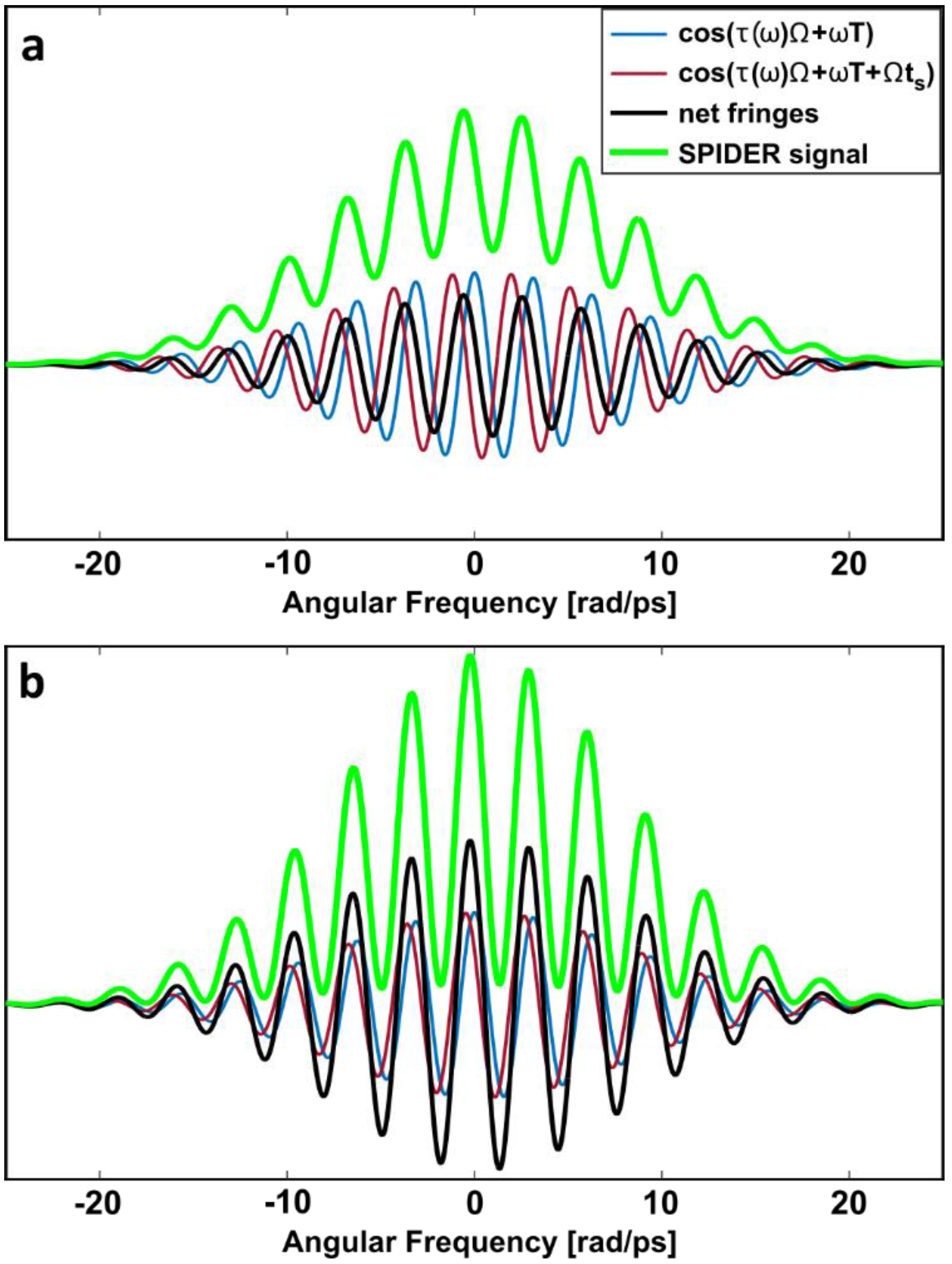
The first two terms above describe the SPIDER trace’s overall intensity envelope. This envelope contains spectral oscillations characteristic of a double pulse. The remaining four terms describe the SPIDER signal’s interference fringes. The first two oscillatory terms are typical fringes that would appear in common SPIDER measurements of each single pulse. As in all SPIDER measurements, each individual pulse interferes with a spectrally sheared replica of itself, creating fringes that are a function of the group delay. The second pair of fringe terms depend on both pulses in the double pulse. Here the first of the two pulses interferes with the sheared replica of the second pulse, and the second pulse interferes with the sheared replica of the first pulse. These fringe terms have different periodicities due to the different relative delays, and they also depend on the relative phase θ between the two pulses.
If θ varies randomly from 0 to 2 π , then in an averaged measurement some of the terms in Equation (4) would average to zero. Specifically, the spectral modulations in the envelope even out and the last two fringe terms disappear. In this case, the SPIDER-trace expression the simplifies to:
S S P I D E R | E ( ω ) | 2 + | E ( ω + Ω ) | 2 + | E ( ω ) | | E ( ω + Ω ) | · { cos ( τ ( ω ) Ω + ω T ) + cos ( τ ( ω ) Ω + ω T + Ω t s ) }
Notice that this expression differs only slightly from the general expression for SPIDER in Equation (2). In this expression there are two sets of fringes instead of just one. The two fringe terms are nearly identical and only differ by a factor of Ω t s (the pulse separation times the spectral shear). To put the spectral shear in context, the temporal range in a SPIDER measurement is 2 π / Ω . Ω t s is therefore 2 π times the ratio of the pulse separation and the SPIDER temporal range. The second fringe term has a phase offset from the first fringe term that is proportional to how large the pulse separation is compared to the temporal range of the SPIDER measurement. This ratio depends on both the pulse’s characteristics and the device parameters.
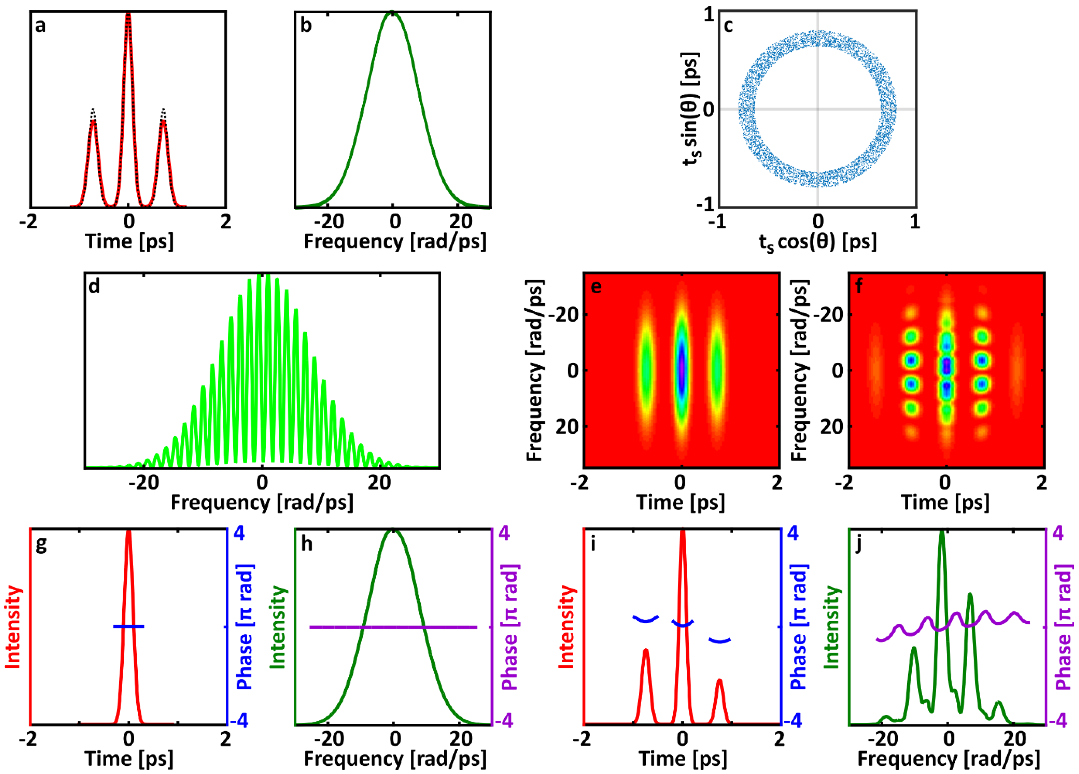
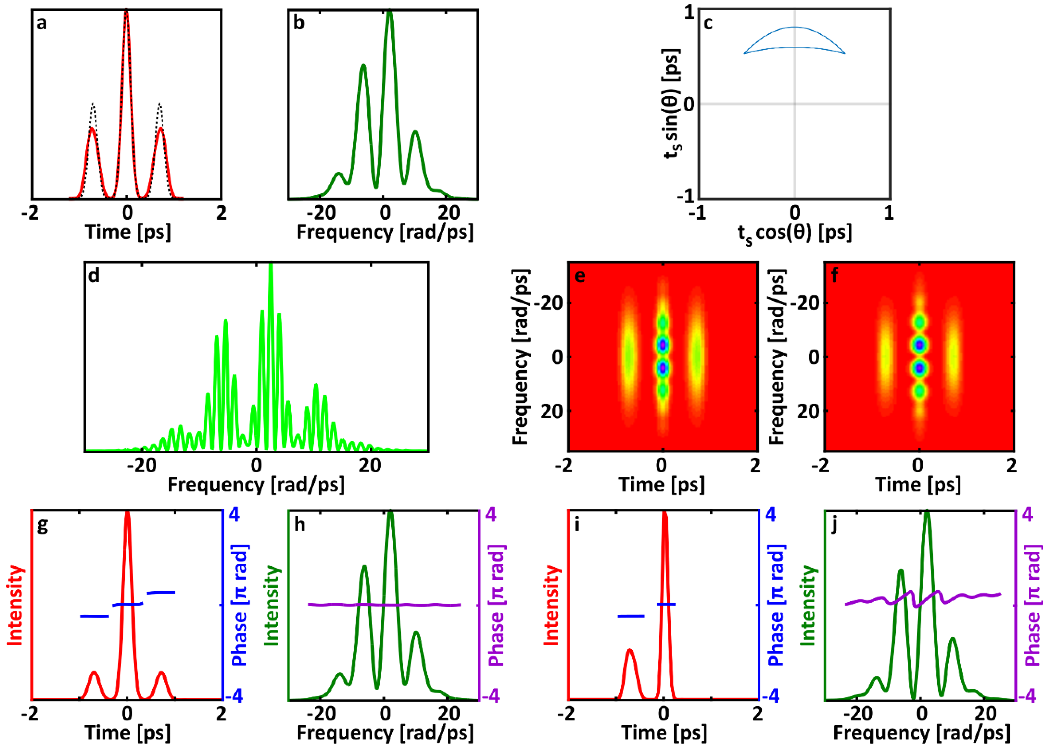
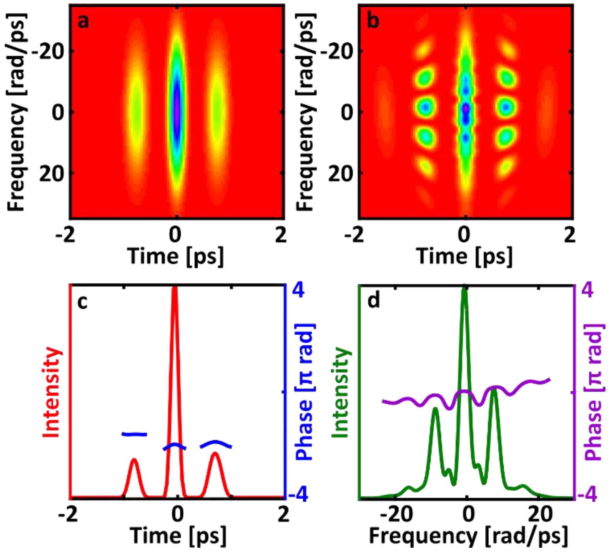
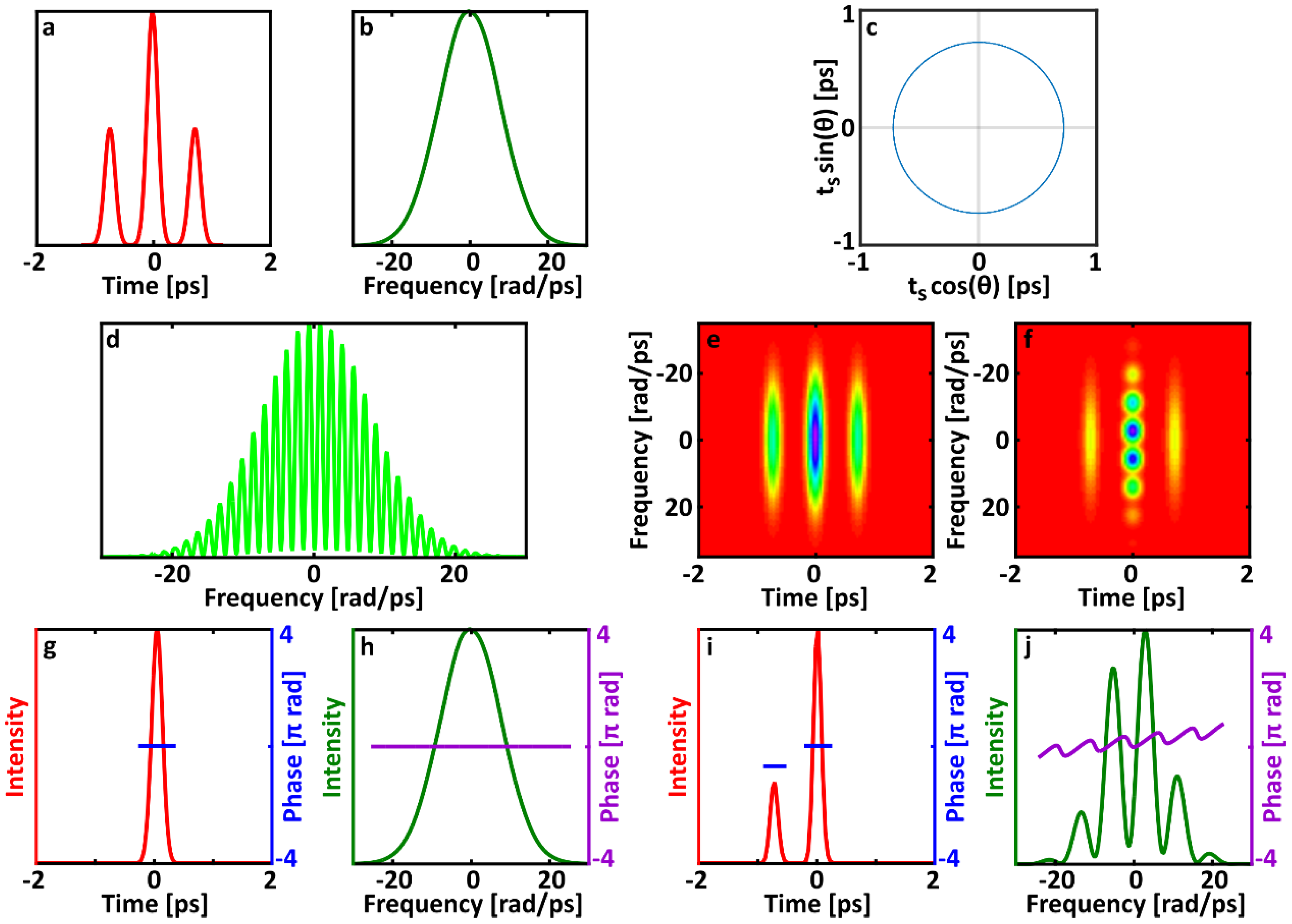
When the pulse separation is stable, there is a consistent phase offset between the fringes. Because the fringe terms are otherwise identical, their sum gives the same group delay as the individual terms. Thus, if the relative phase between the two pulses varies randomly, SPIDER will interpret double pulses as a single pulse with the temporal width of one of the individual pulses. In other words, ones of the pulses will be ignored completely. The size of the phase offset, which is controlled by the ratio of the pulse separation to the temporal support, determines how much background is present in the trace. If the separation between pulses is small compared to the temporal range (that is, support), then the sum of the two fringe terms cannot be distinguished from a single cosine and has almost no background. As the pulse separation increases, the fringe terms are less in phase and the background increases (see Figure 2). Regardless of the amount of background, a SPIDER measurement of a double pulse with varying relative phase will always yield a single pulse. What is particularly interesting about this case is that it is possible to have very good fringe visibility and still have a very wrong measurement. In contrast with studies of other types of unstable pulses in SPIDER, having very low background is not a guarantee of measuring a pulse correctly.
If the pulse separation is not stable, then the phase offset between the two fringe terms is variable. There will be partial cancellation of fringes from the unstable pulse and some background present. As found previously, the fringes from the second pulse will vanish from the measurement if its relative arrival time varies by the temporal support.
In real SPIDER measurements, there is another issue that may affect how double pulses are measured. Because the spectral shear experienced by the pulse replicas is generated by interacting with different parts of an extremely chirped pulse, parts of the pulse occurring at different times will experience slightly different frequencies. While the frequency difference between the original pulse and the replica should remain constant in time, a double pulse will end up with slightly different frequencies for both pulses in the original pulse-shape and for both pulses in the replica. The modified expression for the SPIDER signal is:
S S P I D E R | E ( ω ) + E ( ω + Ω ) exp ( i ω T ) + E ( ω + δ ) · exp ( i θ + i ω t s ) + E ( ω + Ω + δ ) · exp ( i ω T + i θ + i ( ω + Ω ) t s ) | 2
where δ = Ω t s T is the difference in shear experienced by the two pulses in the double pulse. Compared to Equation (3), both the second pulse and its sheared replica experience an additional shear of δ . This is not likely to have a large impact on the measurement, and this effect is not taken into account by the typical SPIDER retrieval procedure.
However, we have included the differences in shear for individual pulses in our simulations to obtain a more accurate approximation for the actual measurement process. Interestingly, comparing the averaged SPIDER traces in Figure 3, Figure 4 and Figure 5 to previous simulations of double pulses in SPIDER [18] shows that adding the differences in shear has essentially no impact on the SPIDER signal in this situation.

2.2. Double Pulses in FROG

General analytical consideration of FROG traces is usually impractical because expressions for self-referenced spectrograms tend to be quite complicated. Considering double pulses is simpler, however, and, assuming that the two pulses are both flat-phase Gaussians simplifies the calculation further. While these assumptions are restrictive, the resulting calculation is still quite informative for more general situations. Writing the time-domain electric field for a Gaussian double pulse:
E ( t ) = exp ( t 2 / σ t 2 ) + exp ( ( t + t s ) 2 / σ t 2 + i θ )
the corresponding SHG FROG measurement is:
I S H G   F R O G ( ω , T ) = | E ( t ) E ( t T ) exp ( i ω t ) d t | 2
= | [ exp ( t 2 σ t 2 ) + exp ( ( t + t s ) 2 σ t 2 ) ] · [ exp ( ( t T ) 2 σ t 2 ) + exp ( ( t + t s T ) 2 σ t 2 ) ] exp ( i ω t ) d t | 2
where T is again the delay between pulse replicas. After some calculations, this expression becomes:
I S H G   F R O G ( ω , T ) exp ( T 2 σ t 2 ) exp ( ω 2 σ t 2 4 ) [ cos 2 ( ω t s 2 + θ ) + 2 cos ( ω t s 2 + θ ) exp ( t s 2 2 σ t 2 ) cosh ( t s T σ t 2 ) + 2 exp ( t s 2 σ t 2 ) + exp ( t s 2 σ t 2 ) cosh ( 2 t s T σ t 2 ) ]
The second and third terms inside the brackets are negligibly small because the pulse separation t s is typically larger than σ t . The last (fourth) term can be written in a more intuitive form, resulting:
I S H G   F R O G ( ω , T ) exp ( T 2 σ t 2 ) exp ( ω 2 σ t 2 4 ) cos 2 ( ω t s 2 + θ ) + 1 2 exp ( ω 2 σ t 2 4 ) [ exp ( ( T t s ) 2 σ t 2 ) + exp ( ( T + t s ) 2 σ t 2 ) ]
This expression describes the archetypal SHG FROG trace for double-pulses. The Gaussian frequency and delay amplitudes are equivalent to the FROG trace for a simple flat-phase Gaussian pulse. As is the case for all FROG traces of double-pulses, spectrogram has three intensity lobes, centered at T = 0 and T = ± t s respectively. The middle lobe (the first term) has fringes that depend on the pulse separation as well as relative phase. The side lobes are half as intense as the center lobe but have the same temporal and spectral widths as does the center lobe.
Allowing the relative phase θ to vary freely erases the fringes in the center lobe of the trace (see, for example, Figure 3e). Significantly, the resulting trace, with three smooth (fringeless) lobes, which is the sum of many different traces corresponding to the many different double-pulse relative phases, is not a valid FROG trace for any pulse, no matter how complex. This is because the trace constrains both the temporal and spectral structure of the integrated electric field over many different pulses. Lobes separated in delay in a FROG trace clearly require the field to have satellite pulses, as in intensity autocorrelation. However, important for our purposes, stable satellite pulses also cause spectral fringes, and therefore the FROG trace should have frequency fringes in the center lobe. In fact, double pulses are used for calibration of the frequency axis in FROG for exactly this reason. Equivalently, the spectral structure of the FROG trace is constrained by the fact that the autoconvolution of the pulse spectrum must be equal to the frequency marginal (the sum of the trace over delay) [11]. Integrating the smooth averaged trace over delay—computing the frequency marginal—yields a spectral profile that is smooth. Thus, the lack of spectral structure in the trace requires the spectrum to be smooth, but the temporal structure requires the pulse spectrum to be modulated. There is no electric field that satisfies both conditions. Consequently, the averaged FROG trace of double pulses with varying relative phase cannot correspond to any single pulse. This is a very useful and important feature of FROG—this discrepancy indicates the presence of instability. Indeed, such discrepancies were also found to occur in the presence of partial mode-locking in our previous work and so meant that FROG is a good indicator of that type of instability. This works because the FROG trace is two-dimensional, whereas the pulse is only one-dimensional, and the resulting over-determination of the pulse by the trace yields this additional information.
In the case of unstable double-pulsing, a variable pulse separation causes the position of the side lobes to vary. It also causes variations the periodicity of the fringes in the center lobe. Averaging over a range of pulse separations results in less intense, temporally wider side lobes in the averaged trace. Broadening the side lobes also causes the trace to become invalid for a single electric field. The spectrum of the side lobes is unchanged, but becoming longer in time with an equally broad spectrum requires consequently the addition of some phase variations, such as chirp. However, since the central lobe does not become wider in time, the field must also be nearly transform-limited. Variations in either pulse separation or relative phase lead to measured traces that are impossible to match with a single electric field. As a result, the FROG pulse-retrieval algorithm responds to these averaged spectrograms of unstable pulses cannot be predicted and is best studied using simulations.
On the other hand, the averaged SHG FROG trace still contains a significant amount of information about the ensemble of double pulses. In particular, the SHG FROG trace of a double pulse is easily recognized, and the lack of fringes in the central lobe is a clear indicator that there are variations in the relative phase of the second pulse. This allows a simple post-processing technique to find the relative intensity of the satellite pulse. Specifically, the relative energy of the two pulses can always be determined without ambiguity (even if the order in which they arrive is ambiguous) based on the energy contained in each lobe in the trace. Because the side lobes are a cross-correlation between the first and second pulses, their energy is proportional to the product of the energy of each individual pulse. The center lobe contains the autocorrelation of each pulse, and therefore its energy is proportional to the sum of the squares of the energy in each individual pulse. If one pulse has an energy of 1 and the other pulse has relative energy α , we can write expressions for the energy in the center lobe M c and a side lobe M s as:
1 + α 2 M c , α M s
The constants of proportionality are the same for each expression, and the exact energy of the pulses is often not of interest. Consequently, it makes sense to take the ratio of these two expressions. Multiplying through by α and rearranging gives a quadratic expression that is easily solved:
α 2 M c M s α + 1 = 0
The energy in each lobe can be determined by integrating the corresponding sections of the measured FROG trace over frequency and delay. One the ratio of the energies has been found, then this quadratic expression can be solved to yield the relative energy, α , of the second pulse.
Equation (13) holds true even when the relative phase and separation between the two pulses changes. Note that M c and M s refer to the total energy in each lobe, not merely their intensity. Thus, even though changing the separation of the two pulses in the double pulse will change the position of the side lobe, the energy will always be recorded in the trace. The total energy in the side lobes is unchanged, even though their peak intensity is lower when the pulse separation varies. This expression also holds true when the two pulses have different spectra or temporal profiles, although the relationship between the pulse energy and the pulse intensity will be different for each pulse in that case. If the relative energy of the two pulses varies, then the calculated relative energy will be the average relative energy. This very simple analysis can provide an additional check on FROG for double pulses. If the retrieved temporal pulse shape has pulses with a different relative energy from the one derived from the energy in the lobes of the trace, then there is further evidence of instability.
Our simulations will attempt to confirm the FROG post-processing approach presented above and study the FROG algorithm’s response to traces generated from unstable double pulses. With simulations, we can also investigate cases that are difficult to address analytically, such as the presence of small variations in the relative phase or of correlations between the pulse relative phase and separation.

3. Methods

Our simulations average over sets of 5000 pulses. We calculate the appropriate measured trace for each pulse using Equation (6) for SPIDER and Equation (8) for SHG FROG. To create the double pulses, we use flat-phase Gaussian pulses with a temporal full width at half maximum (FWHM) of 150 fs. The temporal grid comprises 4096 points with a spacing of 20 fs. The simulation’s resulting spectral resolution is 0.077 rad/ps. For the SPIDER measurement, the spectral shear was chosen to be 12 frequency steps (0.9 rad/ps) and the delay was chosen to be 4 ps. The temporal support is 6.8 ps for a spectral shear of 0.9 rad/ps. The average separation of the double pulses in the pulse trains varies somewhat between the different cases considered, but is approximately 700 fs overall. Because the average pulse separation (0.7 ps) was much smaller than the temporal range (6.8 ps), our calculations suggest that there should be little fringe cancellation and good fringe visibility in the simulated SPIDER measurements.
We cropped the FROG traces and sampled them to reduce the trace size from 4096 × 4096 to 512 × 512. This trace size is still fairly large compared to experimentally common sizes, so the resulting G errors (rms differences or FROG errors), normalized by the number of points, are smaller than those usually observed. FROG errors for experimental data should usually be less than 0.01, and correct retrievals of noiseless simulated traces should have errors much lower than 0.01.
For the first three cases, we use double pulses with equal energy. We consider double pulses in which only the relative phase varies and a set of pulses in which both the relative phase and the separation vary. For each of these cases, we also generate a plot of the averaged intensity autocorrelation and the average spectrum. In addition, we compute a polar plot of the temporal pulse separation as a function of relative phase between the pulses.

4. Results

4.1. Phase Variation Only

The first case has no variation in the pulse separation. The delay between pulses is set to 720 fs and the relative phase between pulses is allowed to vary freely. The averaged autocorrelation over the whole set of pulses is identical to the autocorrelation of one double pulse (see Figure 3a). The pulse separation as a function of phase is simply a circle (see Figure 3c). The variations in the relative phase between pulses cause the average spectrum to be almost Gaussian (Figure 3b). The average SPIDER trace (Figure 3d) has very little background. The background is expected to be low for this case because the chosen pulse separation is small compared to the temporal support of the measurement. The fringes in the SPIDER trace produce a flat spectral phase (Figure 3h). As a result, the second pulse is invisible (Figure 3g) and the measurement result is a single pulse. The measured FROG trace (Figure 3e) follows the predicted appearance. The retrieved trace (Figure 3f) is visually distinct from the measured trace. Specifically, the retrieved trace has less intense side lobes than the measured trace and has spectral fringes in its center lobe. The G error between measured and retrieved traces is 0.014, which is too large to be acceptable. The retrieved pulse (Figure 3i) has a satellite with the correct temporal separation, but the satellite is much less intense than the satellites in the real pulse train. The retrieved satellite has the same temporal width as the main pulse and a relative energy and intensity of 0.34. The relative pulse energy calculated from the energy of lobes in the measured trace is 1.00, in excellent agreement with the actual relative energy of the pulses.

4.2. Phase and Separation Variation

The second case allows variations in temporal pulse separation in addition to variations in relative phase. The pulse separation varies uniformly by slightly more than the FWHM pulse width—from 640 to 800 fs. Plotting the pulse separation as a function of phase results in a diffuse circle with an inner radius of 640 fs and an outer radius of 800 fs (see Figure 4c). The average autocorrelation changes very little (see Figure 4a). The side lobes are slightly broadened and their height is reduced by a small amount. Interestingly, despite varying the pulse separation by a little more than a pulse width, the width of the side lobes in the autocorrelation has not increased by very much. As in the first case, the average spectrum is close to Gaussian because of the relative-phase variations.
The average SPIDER trace for this case is extremely similar to the average trace for the previous case. The SPIDER measurement again does not see the satellite pulse at all in the averaged measurement. There is almost no background in the SPIDER trace. The averaged measured FROG trace has slightly wider side lobes, similar to the lobe broadening of the autocorrelation. The retrieved FROG trace has a different structure from the measured trace, with an extra pair of faint outer side lobes (see Figure 4f) that indicate the presence of a third satellite (see Figure 4i). The G error is 0.0124. The total energy in the retrieved satellite pulses is significantly less than the energy of the main pulse. Their relative energies are 0.44 and 0.25, for a combined relative energy in satellites of 0.69. Of course, the actual pulses are equal energy double pulses, and relative pulse energy derived from the measured trace is 0.97. Even though the side lobes in the measured trace are broadened by the variation in pulse separation, the relative energy in the two pulses is calculated with good accuracy. Each satellite is temporally separated from the main pulse by an amount equal to the average pulse separation in the actual pulse train (720 fs). The retrieved pulses have a small spectral chirp and have relative phases of approximately π / 6 , 0 , and 2 π / 3 respectively. Running the FROG retrieval many times (using different initial guesses) generates retrieved pulses that all have very similar structure and nearly identical G errors. Some retrievals have positive chirp and some have negative chirp, and the ordering of the intensity and relative phase of satellites varies due to the SHG time direction ambiguity. The general structure is quite consistent, however. The retrieved pulse separations are always equal to the correct average separation of the double pulses measured.

4.3. Small, Correlated Phase and Separation Variation

While many reports of unstable multi-pulsing do not explicitly discuss relative phase, it is likely that the relative phase is usually random. Some simulations show that, under certain unusual conditions, the phase and the separation between pulses can vary together in interesting ways [19]. To explore this type of scenario, we include a third test case where the phase varies over a range of less than 2π and follows a specific path as the pulse separation changes (see Figure 5c). The temporal separation ranges from 590 to 800 fs while the relative phase varies from π / 4 to 3 π / 4 . This is case contains a larger range of separations than earlier cases, and the side lobes in its autocorrelation are broader and less intense as a result. The average spectrum is quite modulated due to the small range of relative phases.
The average SPIDER trace of this pulse train also has an envelope that is strongly modulated, but the spectral phase retrieved from the trace is nearly flat. The retrieved temporal pulse shape has two very low-intensity satellite pulses with relative phases of π / 2 and π / 2 separated from the main pulse by 700 fs, which is the average separation of the double pulses in the pulse train. The measured FROG trace does have fringes in the center lobe, but they are blurred by the variations in relative phase. The side lobes in the measured trace are more diffuse than in previous cases because of the larger range of temporal pulse separations. The retrieved trace appears much more similar to the measured trace than in previous cases, but there are still clear discrepancies between the two. The retrieved time-domain pulse shape includes a small satellite separated by about 700 fs with a relative phase of π / 2 . Interestingly, this satellite pulse has a different temporal width from the main pulse, unlike retrieved satellites for other cases. This retrieved satellite is significantly wider, with a FWHM width of about 250 fs rather than 150 fs. The difference in temporal widths is also visible in the retrieved spectrum, which is more deeply modulated in the middle than at the edges because the spectrum of the satellite is narrower. Despite the longer retrieved satellite pulse, the side lobes in the retrieved trace are still narrower than the side lobes in the measured trace. Energy analysis of the trace gives a relative energy of 0.98 between the pulses. In contrast, the satellite in the retrieved pulse has a relative energy of 0.46. Even though the FROG algorithm does not give the correct relative energy, that information is still present in the measured FROG trace.

4.4. Less Intense Satellite

In order to further test the ability of the proposed FROG post-processing approach to yield the relative intensity of satellites from the measured trace, we include an additional case for FROG only (no such post-processing appears possible in SPIDER because the measured SPIDER trace of an unstable double-pulse is identical to that of a single pulse). In this case, we chose the second-pulse relative energy and intensity to be 0.43 and allowed its separation from the main pulse to vary from 600 to 900 fs. The range of pulse separations in this case is larger than in the other cases considered in this paper. The averaged FROG trace and retrieval is shown in Figure 6. FROG retrieves two low-intensity satellite pulses, but this is clearly not the correct pulse because there are no fringes in the side lobes of the measured trace. Indeed, the measured trace is clearly that of a double pulse, except that the central-lobe fringes are missing—indicating the presence of instability in the relative phase. Post-processing of the trace is then in order, and it correctly yields a relative energy of the second pulse is 0.43, despite the confusion of our FROG algorithm. As an aside, we should mention that, in principle, a new, improved FROG algorithm, trained to recognize such unstable pulse trains, should be possible.

5. Conclusions

Using calculations and simulations, we show that, in the presence of double-pulsing, the SPIDER technique cannot see a second pulse at all when its relative phase varies from 0 to 2 π . This conclusion holds regardless of whether the temporal separation of the two pulses varies. Thus, SPIDER is utterly incapable of guaranteeing that the output of a laser is free of double-pulsing since multi-pulse averaged measurements are nearly always used.
In addition, even very small variations in the pulse relative phase result in SPIDER significantly underestimating the intensity of any satellite pulses. Thus, it will be extremely difficult to see even a slightly random satellite pulse if SPIDER is used for the measurement.
While SHG FROG tends to underestimate their amplitude, satellite pulses are clearly visible in SHG FROG measurements. Such satellites retrieved from SHG FROG traces accurately yield the correct average of the pulse separation if and when it varies. There are also clear structural differences between measured and retrieved FROG traces when pulse-train instability is present. Specifically, their average discrepancy (error) is large compared to that of a quality measurement. Such a large discrepancy is a clear indication of instability, as is also the case for other types of pulse instability. (Interestingly, for many years, such discrepancies were erroneously blamed on “non-convergence” of the FROG algorithm).
We also find that simple observation of the measured and retrieved FROG traces provides clear indications of the measured pulses. For example, the three-lobed trace structure is a clear indication of double pulsing, and missing center-lobe fringes is also a clear indication of relative-phase instability. As an example, we demonstrate that the relative energy of the two pulses in the double pulse can be retrieved from the trace directly, even when the temporal separation of the two pulses is not stable. We conclude that comparing the measured and retrieved traces allows FROG users to have much greater confidence in whether instability is present in their lasers, and therefore to have greater confidence in the correctness of their measurement.

Acknowledgments

Some of the results in this manuscript have been published in the SPIE Proceedings 9732, and text and figures from that article have been reproduced herein. Financial support is from the US National Science Foundation Grants #ECCS-1307817 and #ECCS-1609808 and the Georgia Research Alliance. This work was performed in part under the auspices of the U.S. Department of Energy by Lawrence Livermore National Laboratory under Contract DE-AC52-07NA27344.

Author Contributions

Rick Trebino conceived the research and suggested and oversaw the simulations. Michelle Rhodes and Zhe Guang performed the simulations. Michelle Rhodes wrote the paper with help from Rick Trebino and Zhe Guang.

Conflicts of Interest

Rick Trebino owns a company that manufactures pulse-measurement devices.

References

  1. Zipfel, W.R.; Williams, R.M.; Webb, W.W. Nonlinear magic: Multiphoton microscopy in the biosciences. Nat. Biotechnol. 2003, 21, 1369–1377. [Google Scholar] [CrossRef] [PubMed]
  2. Hell, S.W.; Wichmann, J. Breaking the diffraction resolution limit by stimulated emission: Stimulated-emission-depletion fluorescence microscopy. Opt. Lett. 1994, 19, 780–782. [Google Scholar] [CrossRef] [PubMed]
  3. Fleming, G. Chemical Applications of Ultrafast Spectroscopy; Oxford University Press: New York, NY, USA, 1986. [Google Scholar]
  4. Nechay, B.; Siegner, U.; Achermann, M.; Bielefeldt, H.; Keller, U. Femtosecond pump-probe near-field optical microscopy. Rev. Sci. Instrum. 1999, 70, 2758–2764. [Google Scholar] [CrossRef]
  5. Fisher, R.A.; Fleck, J.J.A. On the phase characteristics and compression of picosecond light pulses. Appl. Phys. Lett. 1969, 15, 287–290. [Google Scholar] [CrossRef]
  6. Van Stryland, E.W. The effect of pulse to pulse variation on ultrashort pulsewidth measurements. Opt. Commun. 1979, 31, 93–96. [Google Scholar] [CrossRef]
  7. Ratner, J.; Steinmeyer, G.; Wong, T.C.; Bartels, R.; Trebino, R. Coherent artifact in modern pulse measurements. Opt. Lett. 2012, 37, 2874–2876. [Google Scholar] [CrossRef] [PubMed]
  8. Rhodes, M.; Steinmeyer, G.; Ratner, J.; Trebino, R. Pulse-shape instabilities and their measurement. Laser Photonics Rev. 2013, 7, 557–565. [Google Scholar] [CrossRef]
  9. Rhodes, M.; Steinmeyer, G.; Trebino, R. Standards for ultrashort-laser-pulse-measurement techniques and their consideration for self-referenced spectral interferometry. Appl. Opt. 2014, 53, D1–D11. [Google Scholar] [CrossRef] [PubMed]
  10. Rhodes, M.; Mukhopadhyay, M.; Birge, J.; Trebino, R. Coherent artifact study of two-dimensional spectral shearing interferometry. J. Opt. Soc. Am. B 2015, 32, 1881–1888. [Google Scholar] [CrossRef]
  11. Trebino, R. Frequency-Resolved Optical Gating: The Measurement of Ultrashort Laser Pulses; Kluwer Academic Publishers: Dordrecht, The Netherlands, 2002. [Google Scholar]
  12. Iaconis, C.; Walmsley, I.A. Spectral phase interferometry for direct electric-field reconstruction of ultrashort optical pulses. Opt. Lett. 1998, 23, 792–794. [Google Scholar] [CrossRef] [PubMed]
  13. Shlizerman, E.; Ding, E.; Williams, M.O.; Kutz, J.N. The proper orthogonal decomposition for dimensionality reduction in mode-locked lasers and optical systems. Int. J. Opt. 2011, 2012, 831604. [Google Scholar] [CrossRef]
  14. Wu, J.; Cai, H.; Han, X.; Zeng, H. Multi-pulse operation of a Kerr-lens mode-locked femtosecond laser. Chin. Opt. Lett. 2008, 6, 76–78. [Google Scholar]
  15. Kitano, H.; Kinoshita, S. Stable multipulse generation from a self-mode-locked Ti:sapphire laser. Opt. Commun. 1998, 157, 128–134. [Google Scholar] [CrossRef]
  16. Bale, B.G.; Kieu, K.; Kutz, J.N.; Wise, F. Transition dynamics for multi-pulsing in mode-locked lasers. Opt. Express 2009, 17, 23137–23146. [Google Scholar] [CrossRef] [PubMed]
  17. Cundiff, S.T.; Soto-Crespo, J.M.; Akhmediev, N. Experimental evidence for soliton explosions. Phys. Rev. Lett. 2002, 88, 073903. [Google Scholar] [CrossRef] [PubMed]
  18. Rhodes, M.; Guang, Z.; Trebino, R. Unstable multipulsing can be invisible to some ultrashort pulse measurement techniques. SPIE Proc. 2016, 9732, 97320R–97320R-7. [Google Scholar]
  19. Lederer, M.; Luther-Davies, B.; Tan, H.; Jagadish, C.; Akhmediev, N.; Soto-Crespo, J. Multipulse operation of a Ti:sapphire laser mode locked by an ion-implanted semiconductor saturable-absorber mirror. J. Opt. Soc. Am. B 1999, 16, 895–904. [Google Scholar] [CrossRef] [Green Version]
Figure 1. Simulated measurements of stable and unstable pulse trains (left) using spectral interferometry for direct electric field reconstruction (SPIDER) (middle) and second-harmonic-generation (SHG) (frequency-resolved optical gating (FROG) (right). Reprinted with permission from [8], WILEY-VCH Verlag GmbH & Co., 2013.
Applsci 07 00040 g001
Figure 2. Fringe terms and SPIDER signal evaluated for equal-energy double pulses with stable pulse separation, averaged over relative phases from 0 to 2 π . The last two fringe terms in (4) average to zero and are not plotted. In (a), the pulse separation and shear are chosen so that Ω t s = 0.75 π . Because the two surviving fringe terms are not in phase, there is some cancellation in their sum and the trace shows some background; In (b), the pulse separation is chosen such that Ω t s = 0.3 π . The fringe terms are much closer to being in phase, and there is a small amount of background in the SPIDER signal.
Applsci 07 00040 g002
Figure 3. SPIDER and FROG measurements of a train of double pulses with stable separation and varying relative phase (case A). (a) The average autocorrelation; (b) Average spectrum of the double pulse train; (c) Polar plot of the pulse separation as a function of relative phase; (d) Average SPIDER measurement of the whole pulse train; (e) Average FROG measurement of the whole pulse train; (f) Retrieved FROG trace with G error 0.0140; (g) Temporal intensity (red) and phase (blue) of the pulse retrieved by SPIDER; (h) Spectral intensity (green) and phase (purple) of the pulse retrieved by SPIDER; (i) Temporal intensity (red) and phase (blue) of the pulse retrieved by FROG; (j) Spectral intensity (green) and phase (purple) of the pulse retrieved by FROG.
Applsci 07 00040 g003
Figure 4. SPIDER and FROG measurements of a train of unstable double pulses with varying separation and relative phase (case B). (a) The average autocorrelation is shown in red, and the black dotted line shows the autocorrelation of a pulse with an average separation; (b) Average spectrum of the double pulse train; (c) Polar plot of the pulse separation as a function of relative phase; (d) Average SPIDER measurement of the whole pulse train; (e) Average FROG measurement of the whole pulse train; (f) Retrieved FROG trace with G error 0.0124; (g) Temporal intensity and phase of the pulse retrieved by SPIDER; (h) Spectral intensity and phase of the pulse retrieved by SPIDER; (i) Temporal intensity and phase of the pulse retrieved by FROG; (j) Spectral intensity and phase of the pulse retrieved by FROG.
Applsci 07 00040 g004
Figure 5. SPIDER and FROG measurements of a train of unstable double pulses with correlated separation and relative phase (case C). (a) The average autocorrelation is shown in red, and the black dotted line shows the autocorrelation of a pulse with an average separation; (b) Average spectrum of the double pulse train; (c) Polar plot of the pulse separation as a function of relative phase; (d) Average SPIDER measurement of the whole pulse train; (e) Average FROG measurement of the whole pulse train; (f) Retrieved FROG trace with G error 0.0016; (g) Temporal intensity and phase of the pulse retrieved by SPIDER; (h) Spectral intensity and phase of the pulse retrieved by SPIDER; (i) Temporal intensity and phase of the pulse retrieved by FROG; (j) Spectral intensity and phase of the pulse retrieved by FROG.
Applsci 07 00040 g005
Figure 6. FROG measurement of a train of pulses with an unstable lower intensity satellite pulse. (a) Average FROG measurement of the whole pulse train; (b) Retrieved FROG trace with G error 0.0115; (c) Temporal intensity and phase of the pulse retrieved by FROG; (d) Spectral intensity and phase of the pulse retrieved by FROG.
Applsci 07 00040 g006

