
Measurements and Modeling of the Nonlinear Behavior of a Guitar Pickup at Low Frequencies † †

 ,
,
Abstract
:
1. Introduction
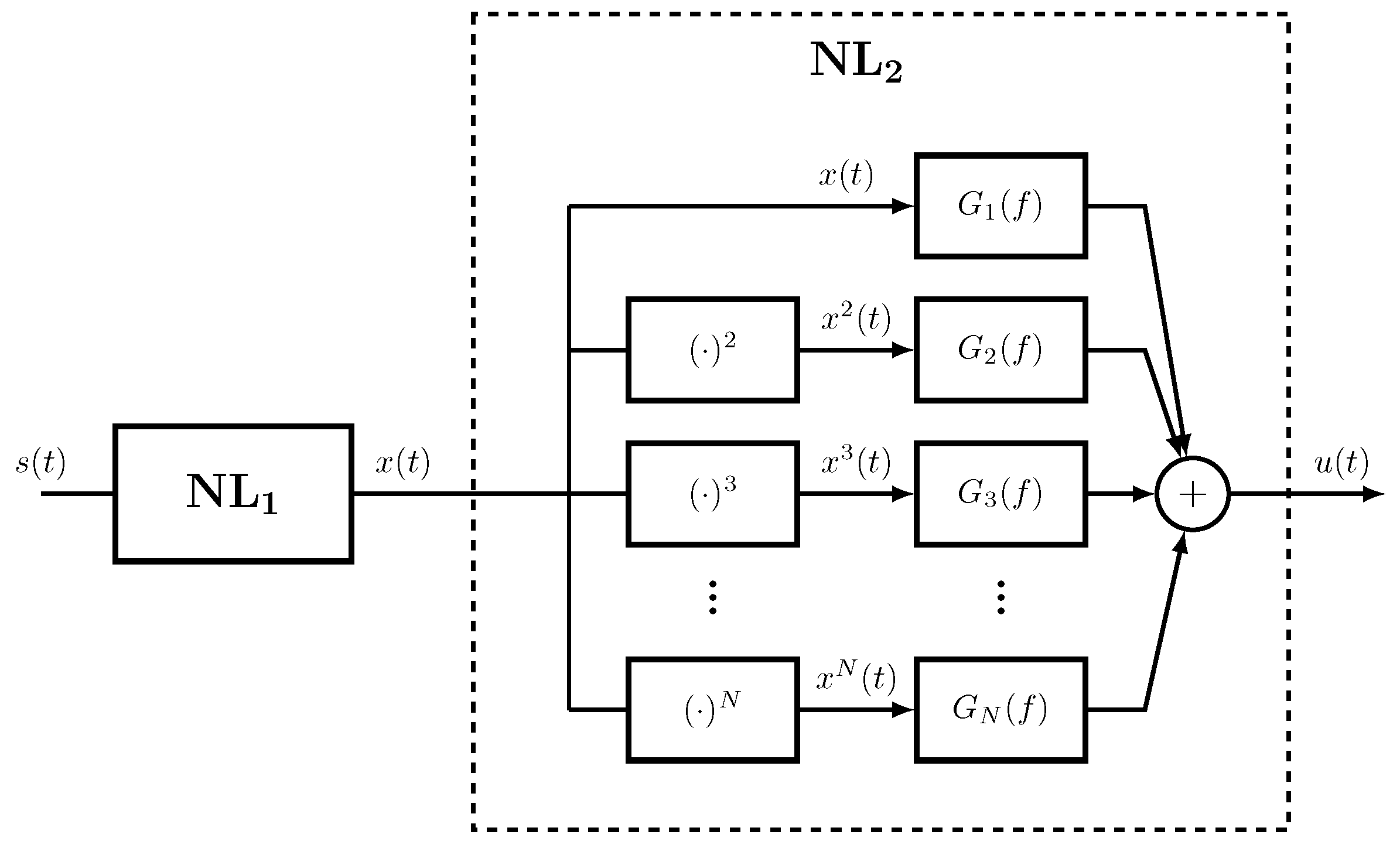
2. Nonlinear Models
3. Synchronized Swept-Sine Technique
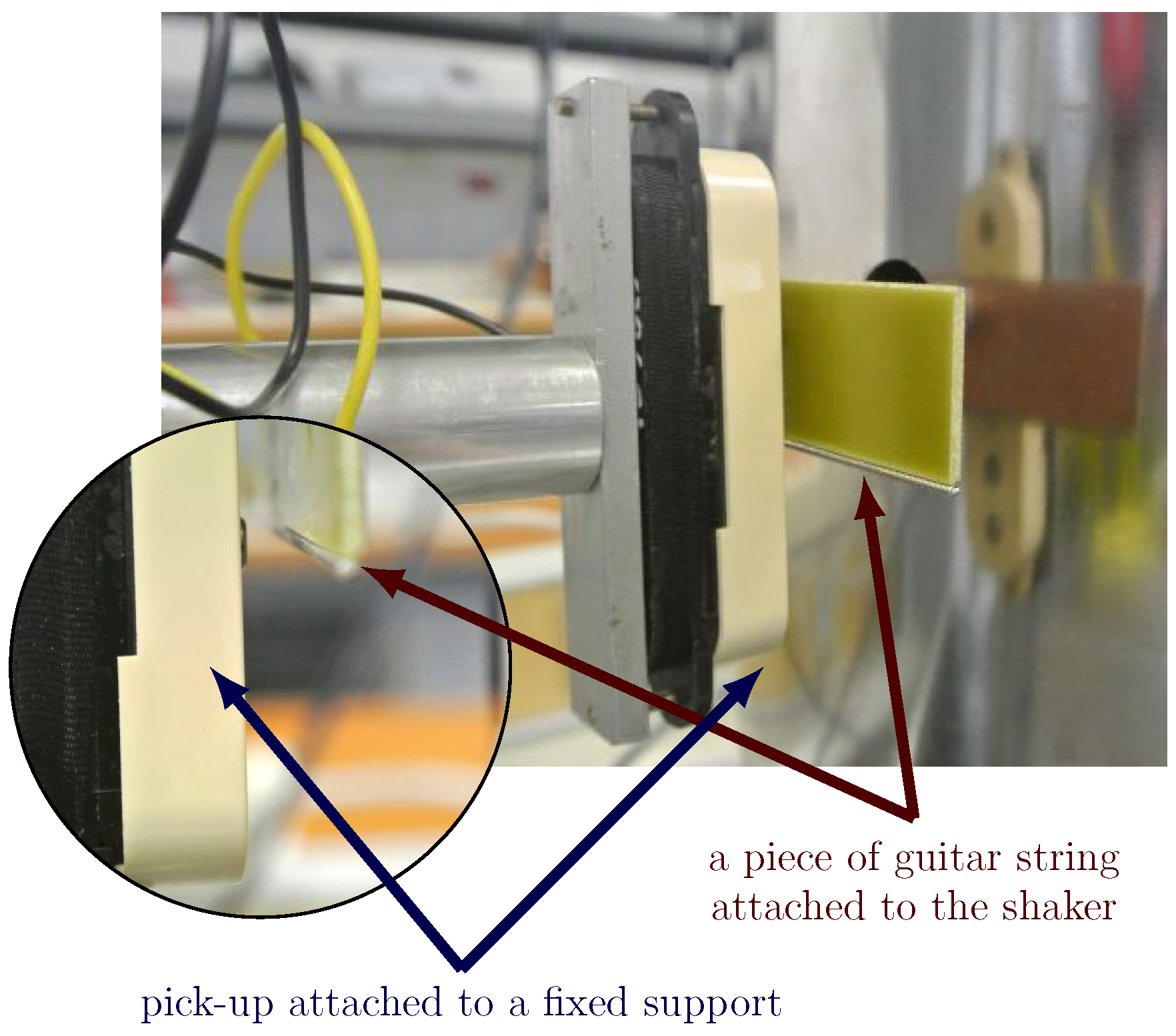
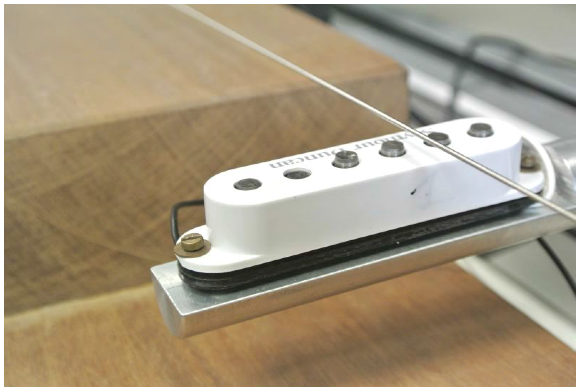
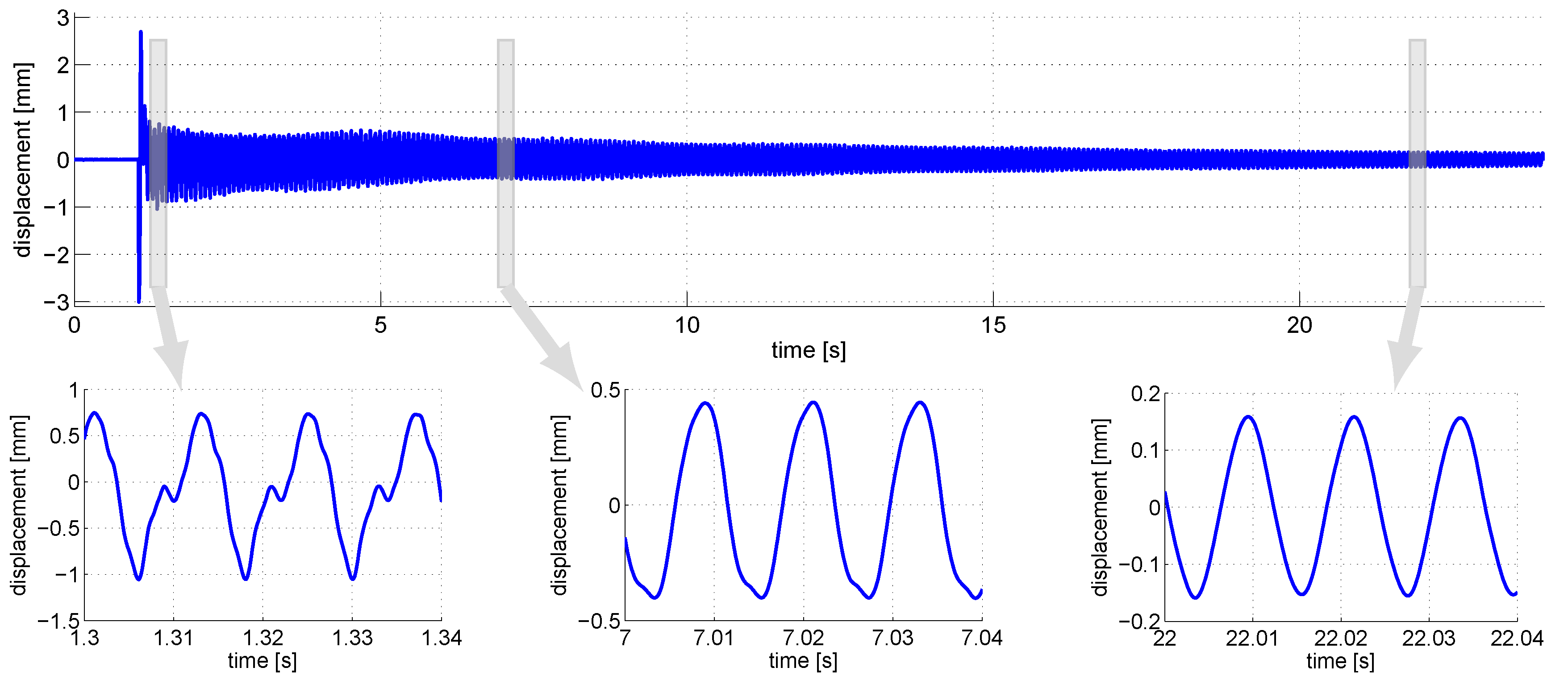
4. Measurement of the Pickup Nonlinearities
5. Nonlinear Parametric Model of the Pickup
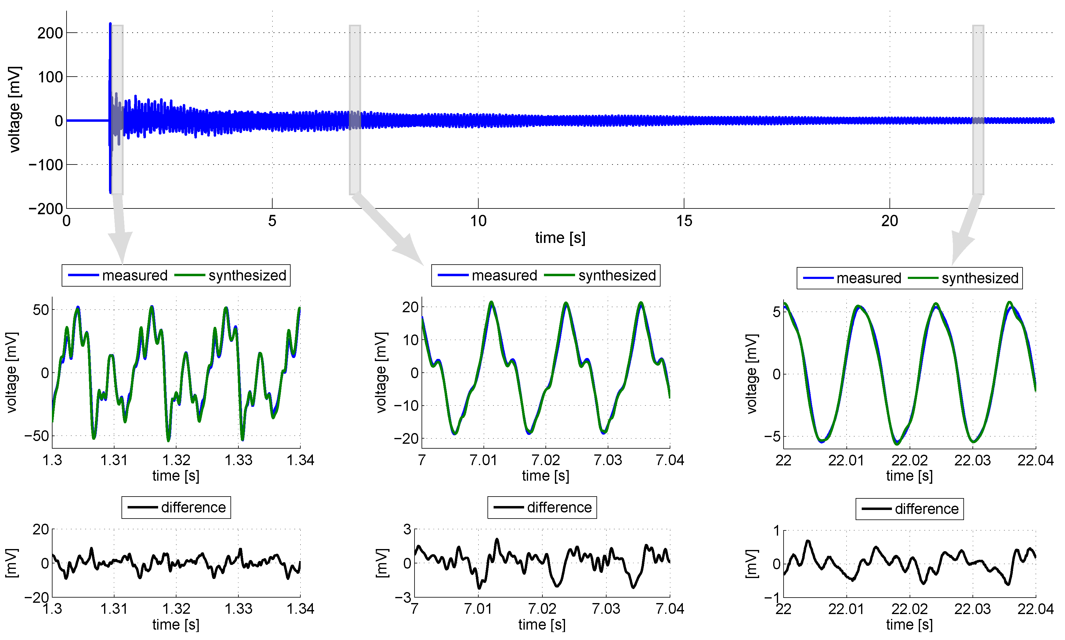
6. Model vs. Real Guitar-String Signal
7. Discussion
8. Conclusions
Acknowledgments
Author Contributions
Conflicts of Interest
Appendix A

References
- Smith, J.O. Physical modeling synthesis update. Comput. Music J. 1996, 20, 44–56. [Google Scholar] [CrossRef]
- Välimäki, V.; Pakarinen, J.; Erkut, C.; Karjalainen, M. Discrete-time modelling of musical instruments. Rep. Prog. Phys. 2005, 69, 1. [Google Scholar] [CrossRef]
- Välimäki, V.; Huopaniemi, J.; Karjalainen, M.; Jánosy, Z. Physical Modeling of Plucked String Instruments with Application to Real-Time Sound Synthesis. J. Audio Eng. Soc. 1996, 44, 331–353. [Google Scholar]
- Laurson, M.; Erkut, C.; Välimäki, V.; Kuuskankare, M. Methods for modeling realistic playing in acoustic guitar synthesis. Comput. Music J. 2001, 25, 38–49. [Google Scholar] [CrossRef]
- Evangelista, G.; Eckerholm, F. Player–instrument interaction models for digital waveguide synthesis of guitar: Touch and collisions. IEEE Trans. Audio Speech Lang. Process. 2010, 18, 822–832. [Google Scholar] [CrossRef]
- Karjalainen, M.; Mäki-Patola, T.; Kanerva, A.; Huovilainen, A. Virtual air guitar. J. Audio Eng. Soc. 2006, 54, 964–980. [Google Scholar]
- Karjalainen, M.; Penttinen, H.; Valimaki, V. Acoustic sound from the electric guitar using DSP techniques. In Proceedings of the 2000 IEEE International Conference on Acoustics, Speech, and Signal Processing (ICASSP’00), Istanbul, Turkey, 5–9 June 2000; Volume 2, pp. II773–II776.
- Paté, A.; Le Carrou, J.L.; Fabre, B. Predicting the decay time of solid body electric guitar tones. J. Acoust. Soc. Am. 2014, 135, 3045–3055. [Google Scholar] [CrossRef] [PubMed]
- Bilbao, S.; Torin, A.; Chatziioannou, V. Numerical modeling of collisions in musical instruments. Acta Acust. Acust. 2015, 101, 155–173. [Google Scholar] [CrossRef]
- Hunter, D. The Guitar Pickup Handbook: The Start of Your Sound; Hal Leonard Corporation: Milwaukee, WI, USA, 2008. [Google Scholar]
- Horton, N.G.; Moore, T.R. Modeling the magnetic pickup of an electric guitar. Am. J. Phys. 2009, 77, 144–150. [Google Scholar] [CrossRef]
- Paiva, R.C.; Pakarinen, J.; Välimäki, V. Acoustics and modeling of pickups. J. Audio Eng. Soc. 2012, 60, 768–782. [Google Scholar]
- Remaggi, L.; Gabrielli, L.; de Paiva, R.; Välimäki, V.; Squartini, S. A pickup model for the Clavinet. In Proceedings of the 15th International Conference on Digital Audio Effects (DAFx-12), York, UK, 17–21 September 2012.
- Falaize, A.; Hélie, T. Guaranteed-passive simulation of an electro-mechanical piano: A port-Hamiltonian approach. In Proceedings of the 18th International Conference on Digital Audio Effects (DAFx-15), Trondheim, Norway, 30 November–3 December 2015.
- Falaize, A.; Hélie, T. Passive simulation of the nonlinear port-Hamiltonian modeling of a Rhodes Piano. J. Sound Vib. 2017, 390, 289–309. [Google Scholar] [CrossRef]
- Novak, A.; Simon, L.; Kadlec, F.; Lotton, P. Nonlinear system identification using exponential swept-sine signal. IEEE Trans. Instrum. Meas. 2010, 59, 2220–2229. [Google Scholar] [CrossRef]
- Rébillat, M.; Hennequin, R.; Corteel, E.; Katz, B.F. Identification of cascade of Hammerstein models for the description of nonlinearities in vibrating devices. J. Sound Vib. 2011, 330, 1018–1038. [Google Scholar] [CrossRef] [Green Version]
- Tronchin, L. The emulation of nonlinear time-invariant audio systems with memory by means of Volterra series. J. Audio Eng. Soc. 2013, 60, 984–996. [Google Scholar]
- Pearson, R.K. Discrete-Time Dynamic Models; Oxford University Press: Oxford, UK, 1999. [Google Scholar]
- Schetzen, M. The Volterra and Wiener Theories of Nonlinear Systems; John Wiley & Sons: New York, NY, USA, 1980. [Google Scholar]
- Rugh, W.J. Nonlinear System Theory; Johns Hopkins University Press: Baltimore, MD, USA, 1981. [Google Scholar]
- Eichas, F.; Möller, S.; Zölzer, U. Block-Oriented Modeling of Distortion Audio Effects Using Iterative minimization External Link. In Proceedings of the 18th International Conference on Digital Audio Effects (DAFx-15), Trondheim, Norway, 30 November–3 December 2015.
- Yeh, D.T.; Abel, J.S.; Smith, J.O. Simplified, physically-informed models of distortion and overdrive guitar effects pedals. In Proceedings of the 10th International Conference on Digital Audio Effects (DAFx-07), Bordeaux, France, 10–15 September 2007; pp. 10–14.
- Eichas, F.; Fink, M.; Holters, M.; Zölzer, U. Physical Modeling of the MXR Phase 90 Guitar Effect Pedal. In Proceedings of the 17th International Conference on Digital Audio Effects (DAFx-14), Erlangen, Germany, 1–5 September 2014; pp. 153–158.
- Kaizer, A.J. Modeling of the nonlinear response of an electrodynamic loudspeaker by a Volterra series expansion. J. Audio Eng. Soc. 1987, 35, 421–433. [Google Scholar]
- Agerkvist, F.T. Volterra Series Based Distortion Effect. In Proceedings of the AES 120th Convention, San Francisco, CA, USA, 4–7 November 2010.
- Ll-Duwaish, H.; Karim, M.N. A new method for the identification of Hammerstein model. Automatica 1997, 33, 1871–1875. [Google Scholar] [CrossRef]
- Koukoulas, P.; Kalouptsidis, N. Blind identification of second order Hammerstein series. Signal Process. 2003, 83, 213–234. [Google Scholar] [CrossRef]
- Chan, K.H.; Bao, J.; Whiten, W.J. Identification of MIMO Hammerstein systems using cardinal spline functions. J. Process Control 2006, 16, 659–670. [Google Scholar] [CrossRef]
- Hélie, T. Volterra series and state transformation for real-time simulations of audio circuits including saturations: Application to the Moog ladder filter. IEEE Trans. Audio Speech Lang. Process. 2010, 18, 747–759. [Google Scholar] [CrossRef]
- Panicker, T.M.; Mathew, V. Parallel-cascade realizations and approximations of truncated Volterra systems. IEEE Trans. Signal Process. 1998, 46, 2829–2832. [Google Scholar] [CrossRef]
- Ji, W.; Gan, W.S. Identification of a parametric loudspeaker system using an adaptive Volterra filter. Appl. Acoust. 2012, 73, 1251–1262. [Google Scholar] [CrossRef]
- Mirri, D.; Luculano, G.; Filicori, F.; Pasini, G.; Vannini, G.; Gabriella, G.P. A modified Volterra series approach for nonlinear dynamic systems modeling. IEEE Trans. Circuits Syst. I 2002, 49, 1118–1128. [Google Scholar] [CrossRef]
- Novak, A.; Simon, L.; Lotton, P.; Gilbert, J. Chebyshev model and synchronized swept sine method in nonlinear audio effect modeling. In Proceedings of the 13th International Conference on Digital Audio Effects (DAFx-10), Graz, Austria, 6–10 September 2010.
- Oksanen, S.; Välimäki, V. Modeling of the carbon microphone nonlinearity for a vintage telephone sound effect. In Proceedings of the 14th International Conference on Digital Audio Effects (DAFx-11), Paris, France, 19–23 September 2011.
- Bank, B. Computationally Efficient Nonlinear Chebyshev Models Using Common-Pole Parallel Filters with the Application to Loudspeaker Modeling. In Proceedings of the AES 130th Convention, London, UK, 13–16 May 2011.
- Novak, A.; Lotton, P.; Simon, L. Synchronized Swept-Sine: Theory, Application, and Implementation. J. Audio Eng. Soc. 2015, 63, 786–798. [Google Scholar] [CrossRef]
- Farina, A.; Bellini, A.; Armelloni, E. Non-Linear Convolution: A New Approach for the Auralization of Distorting Systems. In Proceedings of the AES 110th Convention, Amsterdam, The Netherlands, 12–15 May 2001.
- Mustonen, M.; Kartofelev, D.; Stulov, A.; Välimäki, V. Experimental verification of pickup nonlinearity. In Proceedings of the International Symposium on Musical Acoustics (ISMA 2014), Le Mans, France, 7–12 July 2014; Volume 1.
- Lotton, P.; Lihoreau, B.; Brasseur, E. Experimental Study of a Guitar Pickup. In Proceedings of the International Symposium on Musical Acoustics (ISMA 2014), Le Mans, France, 7–12 July 2014; Volume 1.
- Novak, A.; Maillou, B.; Lotton, P.; Simon, L. Nonparametric identification of nonlinear systems in series. IEEE Trans. Instrum. Meas. 2014, 63, 2044–2051. [Google Scholar] [CrossRef]
- Woodhouse, J. Plucked guitar transients: Comparison of measurements and synthesis. Acta Acust. 2004, 90, 945–965. [Google Scholar]
- Pàmies-Vilà, M.; Kubilay, I.A.; Kartofelev, D.; Mustonen, M.; Stulov, A.; Välimäki, V. High-speed linecamera measurements of a vibrating string. In Proceedings of the Baltic-Nordic Acoustic Meeting (BNAM), Tallinn, Estonia, 2–4 June 2014; Volume 1.
- Pakarinen, J.; Karjalainen, M. An apparatus for measuring string vibration using electric field sensing. In Proceedings of the Stockholm Music Acoustics Conference, Stockholm, Sweden, 6–9 August 2003; pp. 739–742.
- Kotus, J.; Szczuko, P.; Szczodrak, M.; Czyżewski, A. Application of fast cameras to string vibrations recording. In Proceedings of the IEEE Signal Processing: Algorithms, Architectures, Arrangements, and Applications (SPA), Poznań, Poland, 23–25 September 2015; pp. 104–109.
- Novak, A.; Guadagnin, L.; Lihoreau, B.; Lotton, P.; Brasseur, E.; Simon, L. Non-Linear Identification of an Electric Guitar Pickup. In Proceedings of the 19th International Conference on Digital Audio Effects (DAFx-16), Brno, Czech Republic, 5–9 September 2016.


© 2017 by the authors; licensee MDPI, Basel, Switzerland. This article is an open access article distributed under the terms and conditions of the Creative Commons Attribution (CC-BY) license (http://creativecommons.org/licenses/by/4.0/).
Share and Cite
Novak, A.; Guadagnin, L.; Lihoreau, B.; Lotton, P.; Brasseur, E.; Simon, L. Measurements and Modeling of the Nonlinear Behavior of a Guitar Pickup at Low Frequencies †. Appl. Sci. 2017, 7, 50. https://doi.org/10.3390/app7010050
Novak A, Guadagnin L, Lihoreau B, Lotton P, Brasseur E, Simon L. Measurements and Modeling of the Nonlinear Behavior of a Guitar Pickup at Low Frequencies †. Applied Sciences. 2017; 7(1):50. https://doi.org/10.3390/app7010050
Chicago/Turabian StyleNovak, Antonin, Leo Guadagnin, Bertrand Lihoreau, Pierrick Lotton, Emmanuel Brasseur, and Laurent Simon. 2017. "Measurements and Modeling of the Nonlinear Behavior of a Guitar Pickup at Low Frequencies †" Applied Sciences 7, no. 1: 50. https://doi.org/10.3390/app7010050