
Design and Optimization of a Lorentz-Force-Driven Planar Motor

Department of Electrical Engineering, Harbin Institute of Technology, Harbin 150080, China
*
Author to whom correspondence should be addressed.
Appl. Sci. 2017, 7(1), 7; https://doi.org/10.3390/app7010007
Submission received: 5 October 2016
/
Accepted: 16 December 2016
/
Published: 22 December 2016
(This article belongs to the Special Issue Selected Papers from the International Multi-Conference on Engineering and Technology Innovation 2015 (IMETI2015))
Abstract
:This paper describes a short-stroke Lorentz-force-driven planar motor which can realize three-degree-of-freedom motions in high-precision positioning systems. It is an extended version of our previous publication. Based on the analytical model, the force expression concerning the main dimensional parameters is derived. Compared with the finite element simulation, the optimization method in this paper is completely based on the mathematical model, which saves considerable time and has clear physical meaning. The effect of the main parameters on the motor performances such as force, force density, and acceleration are analyzed. This information can provide important design references for researchers. Finally, one prototype is tested. The testing values for the resistance and inductance of the square coil agree well with the analytical values. Additionally, the measured forces show a good agreement with the analytical force expression, and the force characteristics show a good symmetry in the x and y directions.
1. Introduction
In modern high-end manufacturing or testing equipment, such as a wafer stage in a lithography machine, micro/nano positioning platform, and scanning probe microscope, the requirements of the high-precision multi-degree-of-freedom actuating elements are increasing [1,2,3,4,5,6]. Generally, there are three conventional methods to realize multi-degree-of-freedom positioning motions. The first method is the flexure hinge mechanism driven by piezoelectric ceramics [7,8,9]. The second method is to use multiple rotary motors and the corresponding transmission mechanism. The third method is to use multiple linear motors [10,11]. Although the multi-degree-of-freedom motions can be realized using these methods, there are some inevitable defects. For the flexure hinge mechanism and piezoelectric ceramics, it is easy to achieve integral structure and low power loss. However, the damping, micron-grade stroke of the flexure hinge and the hysteresis, non-linear characteristics of the piezoelectric ceramics will limit the performance improvement. For the rotary motor systems, the friction, backlash, and deformation of the transmission mechanism will degrade the positioning accuracy. Additionally, the additional mass of the transmission mechanism is a bottleneck to improve the dynamic performance. For linear motor systems, the positioning accuracy and the dynamic performance is improved due to removal of the transmission chain. However, it still cannot get rid of the mode of superposing low dimensional motions into a high dimensional motion. The bottom motor has to support the top motor. Additionally, a large number of mechanical components leads to a complex structure, which is adverse to further improving the positioning accuracy.
In the last two decades, planar motors brought about a novel and practical solution for industry, and they have been continually receiving more and more attention. A planar motor is a type of motor that can realize planar motion with only one moving part. Planar motors have the features of two-degree-of-freedom (2-D) direct drive, high response, high structural strength, and simple system structure. Therefore, it has broad application prospects in 2-D positioning systems, especially in the high precision applications. According to the working principle, planar motors can be divided into four types, which are reluctance-type planar motor, induction-type planar motor, synchronous-type planar motor, and Lorentz-force-driven planar motor. A planar stepping motor belongs to reluctance-type motors and it is the earliest planar motor [12,13]. A planar stepping motor is comprised of two linear stepping motors. The movers of the two linear stepping motors are integrated into one moving part in mutually perpendicular directions. The stator is a 2-D tooth-slot array. The advantages of the planar stepping motor are no accumulated error and simple structure, but the low frequency oscillation, losing steps, and low speed limit its range of applications. A switched reluctance planar motor is another type of reluctance-type motor, which was proposed by Pan et al. [14,15]. The stator is composed of several blocks, each of which is made of silicon steel sheets instead of solid iron. Therefore, the eddy current effect and the processing cost is reduced. In 1999, Fujii et al. [16] proposed a planar induction motor. The primary is an iron ring winded with windings, and the secondary is a magnetic plate. This motor can achieve not only the long-stroke planar motion, but also the rotary motion. However, there are some disadvantages, such as its complex manufacturing process, low air-gap magnetic flux density, and low operating speed. The 2-D electromagnetic force of the synchronous-type planar motor is from the interaction between a permanent magnet array and coil array. In recent years, this type of planar motors was deeply researched, and many novel topologies were put forward. The earliest synchronous planar motor was proposed by Kim [17], in which there are four groups of linear synchronous units. Each unit can be seen as a slotless linear motor which is composed of a 1-D Halbach magnet array and three-phase windings. In 2002, Cho et al. [18] proposed a new synchronous planar motor, which is composed of a 2-D permanent-magnet array and four 1-D coil arrays. The performances of several 2-D permanent-magnet arrays are compared with each other. In 2007, a novel moving-magnet synchronous planar motor was proposed by Jansen et al. [19]. The motor consists of a 2-D permanent-magnet array and a 2-D coil array. In the 2-D coil array, there are two groups of track-shape coils which are orthogonal and arranged in turn. Obviously, this moving-magnet topology has no moving cables and the heat from a coil array can be easily reduced by adopting cooling solutions.
The above three types of motors are long-stroke planar motors, in which the moving range is usually hundreds of millimeters. However, high-accuracy performance at a millimeter level is often required in many applications. In this case, the Lorentz-force-driven planar motor [20,21,22] is the best solution due to the inherent features of unlimited resolution, high linearity, no force-ripple, etc. Actually, it is more often the case that high accuracy and long stroke are both required in some systems [23,24]. Therefore, the coarse-fine scheme is usually adopted, in which the Lorentz-force-driven planar motor is located on top of the system in order to achieve the precision compensation. The Lorentz-force-driven planar motor needs to be well designed and optimized to simplify the system-level structure and improve the integral dynamic performance, because it lies on the top of the positioning system. Compared with the long-stroke motors at the bottom, the optimization work for the short-stroke motors can do more contributions to the improvement of system performance. At present, the finite element method is usually used in most of the studies in the established literature concerning the design and optimization for planar motors. Obviously, it is a time-consuming method to analyze the planar motors that cannot be completely described by a 2-D finite element model.
In this study, we describe a short-stroke Lorentz-force-driven planar motor. The analytical model containing the air-gap magnetic field, inductance and force expression is built. Based on the model, the main design parameters are determined and the specific influences of the main parameters on motor performances are analyzed. Three important indexes (i.e., the force, force density, and acceleration) are optimized and the reasonable values for the dimensional parameters are concluded. Compared with [1], the main dimensions’ equation is transformed to the force equation in this paper, which is more important for motor optimization. Additionally, the analytical expressions for the force density and acceleration are derived, and the corresponding variation curves are given, which are very important references for this type of motor. Finally, based on the optimization results, reasonable ranges for the main parameters are given, which can balance the force, the force density, and the acceleration for the proposed planar motor.
2. Structure and Working Principle
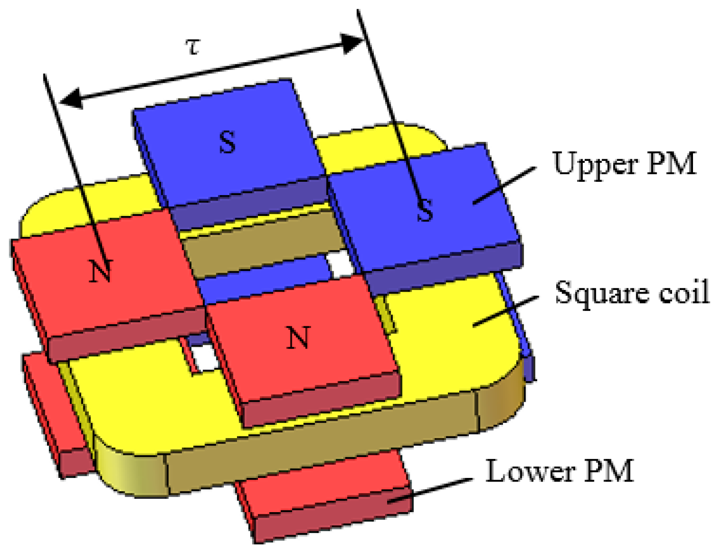
The proposed short-stroke Lorentz-force-driven planar motor, shown in Figure 1, has a moving-magnet scheme, in which the magnet part is the mover (secondary) and the coil part is the stator (primary). The primary is composed of an array of coils, and the secondary is composed of permanent magnets and two back-irons. The four square coils in the primary are controlled by four separate controllers. Compared with round-shaped coils, the effective edges of the square coils in the magnetic field can be fully used, which increases the force level. Actually, the proposed planar motor is combined by four Lorentz-force-driven units. The motor can realize three-degree-of-freedom motion through controlling the current combination of the four driving units. As shown in Figure 2, the Lorentz-force-driven unit consists of three parts: upper magnets, lower magnets, and one square coil. The double-sided structure is adopted to increase the air-gap magnetic field.
The features of the short-stroke planar motor are as follows:
- The working principle is the same as voice coil motors, which is based on the Lorentz force. Compared with three-phase planar motors, with the proposed motor it is easier to achieve high-precision positioning.
- There is no electrical connection and cable disturbance in the moving parts due to the moving-magnet scheme. Additionally, the temperature rise of the motor can be easily controlled because the heat source is in the stator.
- There is no cogging force and force ripple for this slotless motor with air-core coils, which is beneficial for servo performance improvement.
The Lorentz-force-driven unit can be seen as a linear voice coil motor with one square coil. According to the principle of Lorentz force, a force will be generated once an energized conductor is put in the magnetic field. The amplitude and direction of the force is decided by the magnetic flux density, conductor current, and their directions. The Lorentz force equation is written as
where N, I, L, and B are the number of turns, current, conductor length, and magnetic flux density, respectively.
When the magnetic flux density and the conductor are orthogonal, Equation (1) can be written, in the scalar form, as
Upon considering Equation (2), the motor force is dependent on the parameters of the coils and the magnetic field. Due to the correlative relations among different parameters, the optimization design should be taken to achieve the optimal performance of the motor. When conductors move in the magnetic field, the back EMF (Electromotive Force) will be generated, which is in direct proportion to the moving velocity. The power should provide enough current to meet the force target, and conquer the back EMF and the leakage inductance simultaneously. The back EMF equation is written as
where v is the moving velocity.
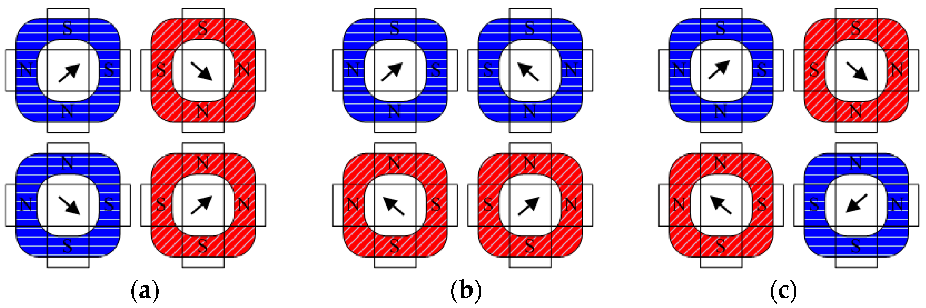
Figure 3 shows the working principle of the Lorentz-force-driven planar motor. The colors (or the stripe in the black-white version) represent the current directions. The blue one (horizontal stripe) represents anticlockwise current, and the red one (slant stripe) represents clockwise current. The arrows represent the force acting on each Lorentz-force-driven unit. Through different force combinations, the planar motor can move in the x, y axis and rotate about the z axis within a small angle.
3. Modeling and Design Optimization
3.1. Magnetic Field and Electromagnetic Force Expression
For the planar motors to be applied in high-precision positioning systems, it is critical to build an accurate mathematical model. Through the model, the main motor parameters can be further optimized. Additionally, excellent control is based on an accurate model. Therefore, modeling is the basis for the motor analysis and optimization.
According to the equivalent magnetic charge method [25,26], a cubic permanent magnet can be represented by two charge surfaces, and the surface density of the magnetic charge is
where μ0 is the vacuum permeability and Mr is the magnetization intensity.
The expression of the magnetic field intensity can be written as
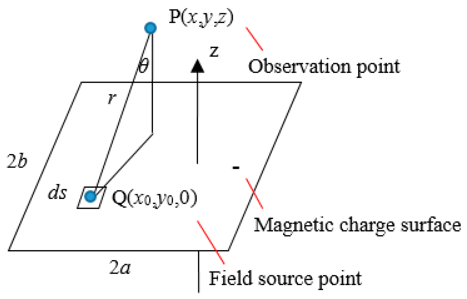
where ar is the unit vector from the field source point to the observation point and r is the distance from the field source point to the observation point, as shown in Figure 4.
The z-axis component of the magnetic field intensity for one charge surface can be expressed as
where x0, y0 are the coordinates of the field source point and 2a, 2b are the length and width of the permanent magnet, respectively.
The final magnetic flux density expression of one cubic magnet can be derived as
where hM is the thickness of permanent magnet.
Due to the existence of double-sided ferromagnetic boundaries, the air-gap magnetic field is not entirely decided by the permanent magnets. Using the image method, superposition principle, and coordinates transformation, the magnetic field expression generated by a couple of magnets under two parallel ferromagnetic boundaries can be derived as
where Bz, original is the magnetic field of original charge and Bz, image is the magnetic field of image charge.
The proposed planar motor is a short-stroke motor, and the working range is about ±2 mm. To simplify the model, the complex magnetic flux density expression can be represented by the amplitude of the magnetic flux density due to the short stroke. The expression of the magnetic flux density amplitude can be derived as
where λ and γ are two main parameters relating to the motor size, the expressions of λ and γ are as follows,
where τ is the pole pitch of the planar motor, as shown is Figure 2, and h is the distance between the upper and lower magnet (i.e., the total thickness of the primary plus two mechanical air gaps). As shown in Figure 2, the square magnets are adopted to guarantee the symmetry of the proposed planar motor. Therefore, the magnet sizes can be fully described only by the pole pitch (τ) and the magnet thickness (hM). Actually, the pole pitch is twice of the length/width of the square magnet (i.e., τ = 4a = 4b).
Once we have obtained the magnetic flux density, we can derive the force expression of the planar motor based on Equation (2). As shown in Figure 3, there are always eight effective sides of the coils which are orthogonal to the moving direction when the motor moves either in the x direction or y direction. Therefore, the force expression is modified to
where lef is the effective length of coil side and can be expressed as
where αi is the pole-arc coefficient.
For the proposed planar motor, which is used in the high-accuracy, high-dynamic systems, a high force level is always required to guarantee the dynamic performance. In general, a large value of h is adopted to provide more space for the coils and to increase the force level. Compared with h, the length of mechanical air-gap is negligible. Therefore, the ampere-turns in Equation (14) can be approximated as
where Jc is the current density of coil cross section and wc is the width of coil, which can be expressed as
where Cfw is the flat top width coefficient. Cfw is defined as the ratio between the width range (W) in which the magnetic flux density B is higher than 0.9Bmax and the pole pitch (i.e., Cfw = W/τ).
Substituting Equations (10) and (15)–(17) into Equation (14), the force expression relating to the main parameters of the planar motor can be derived as
3.2. Optimization Design
3.2.1. Motor force
In Equation (18), the motor force is in direct proportional to τ2h, which reflects the motor volume. In other words, the motor force is decided by the parameters of λ and γ when the motor volume remains constant. As a planar positioning device, the structural stability is important. Therefore, the motor height is always restricted to lower the center of mass. The specific influence of λ and γ on the motor force is analyzed in this part on the condition that the motor height is constant.
Assuming that the motor height is constant, the sum of the magnet height (hM) and the distance between the upper and lower magnet (h) is invariable. The parameter h decreases with the increase of parameter hM. Although the force increases with the increase of hM, it will gradually decrease due to the reduction of the effective conductor region. Figure 5 shows the side view of an effective coil side and the corresponding magnets. The total height of the motor can be written as
Figure 6 shows the force characteristic versus parameter γ. In Figure 6a, the pole pitch remains unchanged. As the motor height increases, the force basically shows a linear increase trend. Additionally, the optimal value of γ in which the force reaches a maximum is always around 0.5. That is to say, the planar motor force increases with the increase of the motor height when the parameter γ is constant and the pole pitch τ equals 50 mm. Additionally, the planar motor force reaches the maximum value when the parameter γ equals 0.5. To see whether the optimal value of γ is universal or not, it needs to be verified by considering the effect of the pole pitch.
Figure 6b shows the force characteristic versus parameter γ with different pole pitches when the total height remains unchanged. It can be seen that the force increases with the increase of the pole pitch, and the optimal value of γ is always around 0.5 no matter what value the pole pitch is. Therefore, the pole pitch can only have an effect on the force, but it cannot affect the optimal value of γ.
3.2.2. Force Density
As a type of short-stroke planar motor, it needs to generate forces as high as possible with a smallest volume (i.e., to achieve an optimal force density). The definition of the force density is the ratio between motor force and volume, which can be written as
where V is the volume of the motor.
To obtain the analytical force density expression, the volume expression is required. The top and side view of the planar motor is shown in Figure 7, and the motor volume, ignoring the back irons, can be obtained as
Substituting Equations (18) and (21) into Equation (20), the force density expression of the planar motor can be derived as
where KG is the force density coefficient.
As shown in Equation (22), the force density of the planar motor mainly depends on the main parameters γ and λ due to the small variation range of the coefficient KG. Figure 8 shows the force density characteristics versus parameters γ and λ, in which the force density variation trend can be found.
In Figure 8a, when the parameter λ is invariant, the force density increases first and then decreases with the increase of parameter γ. There is an optimal value of γ between 0.2 and 0.5. The reason is that, increasing the magnet thickness can increase the air-gap magnetic field and the force, but it also inevitably increases the motor volume. When the value of γ is small, the magnetic field is more sensitive to the magnet thickness rather than the volume, so the force density increases with the increase of γ. However, the force increment will be less than the volume increment when the magnet thickness increases to a certain value, because the force tends to saturate and the volume still increases linearly. Additionally, it can be found that the force density increases with the increase of parameter λ.
In Figure 8b, the force density characteristic with the parameter λ is shown. The force density increases with the increase of parameter λ when the parameter γ is invariant, but the increasing trend gradually becomes saturated. In other words, the force density depends on the shape of the planar motor. The force density is higher in a flat shape than in a high-vertical shape. To obtain the optimal parameters for a maximum force density, the follow equation must be satisfied
3.2.3. Acceleration
For the moving-magnet actuators, the mass of magnets is a major proportion of the total moving mass. Although increasing the quantity of magnets can increase the motor force, it obviously will also increase the moving mass and reduce the dynamic performance of the motor. Therefore, the acceleration can be seen as a main optimization criterion for the proposed planar motor.
Basically, most of the three-degree-of-freedom planar motors are expected to be supported by air bearings. Ignoring the mechanical friction, the equation of acceleration can be written as
where m is the mass of mover.
According to Figure 7, the equation for the mover mass is
where ρM and VM are the density and volume, respectively, for one magnet, and ρj and Vj are the density and volume, respectively, for one back iron.
The equations of VM and Vj are as follows
where hj is the thickness of back iron.
Based on magnetic circuit method, the thickness of back iron can be derived as
where σ0 is the no-load leakage flux coefficient, Br is the remanence of magnet, Bj is the magnetic flux density of back iron, and Ks is the saturation coefficient.
Substituting Equations (18) and (25) into Equation (24), the acceleration expression relating to the main parameters of the planar motor can be derived as
Figure 9 shows the acceleration characteristic versus parameters γ and λ. In Figure 9a, when the parameter λ is invariant, the acceleration decreases with the increase of parameter γ. Additionally, the decreasing trend is obvious when γ < 0.5. In Figure 9b, when the parameter γ is invariant, the acceleration increases first and then decreases with the increase of parameter λ. There is an optimal value of λ around 3 at which the acceleration reaches the maximum value. To obtain the optimal parameters for a maximum acceleration, the follow equation must be satisfied
4. Prototype Experiment and Results
4.1. Resistance and Inductance Test
The model and prototype of the square coil used in the proposed planar motor is shown in Figure 10. The actual sizes of coil and the conductor gauge is given in Table 1.
The resistance calculation formula for the square coil is
where ρ is the resistivity.
Based on Equation (31), the analytical value of the resistance is 2.427 Ω. The actual resistance test results for the four square coils are shown in Table 2.
The estimated value of resistance agrees well with the actual values. The error between them is less than 3.5%. The main reason for the error is that the actual shape of the square coil is slightly different from the one calculated in the model.
The inductance calculation model for the square coil is shown in Figure 11. First, according to the Biot-Savart Law, the magnetic field from one square conductor can be obtained. Then, we can get the magnetic field generated by one square coil with current. Second, the magnetic flux for a single-turn square coil can be calculated with double integral of the magnetic field within the xoy coordinate system. Finally, the total magnetic flux for the square coil with N turns can be calculated using the superposition principle. The inductance calculation formula for the square coil is
Based on Equation (32), the analytical value of the inductance is 4.216 mH. The actual inductance test results for the four square coils are shown in Table 3.
The inductance error between the actual values and the estimated values is about 8%. Although the inductance error is larger compared to the resistance error, it can provide the theoretical basis for the motor design and be beneficial to the parametric modeling due to the analytical expressions.
4.2. Motor Force Test
To verify the model and to test the force characteristic of the proposed planar motor, a prototype motor was manufactured. The prototype parameters are given in Table 4. Figure 12 shows the planar motor force experimental system.
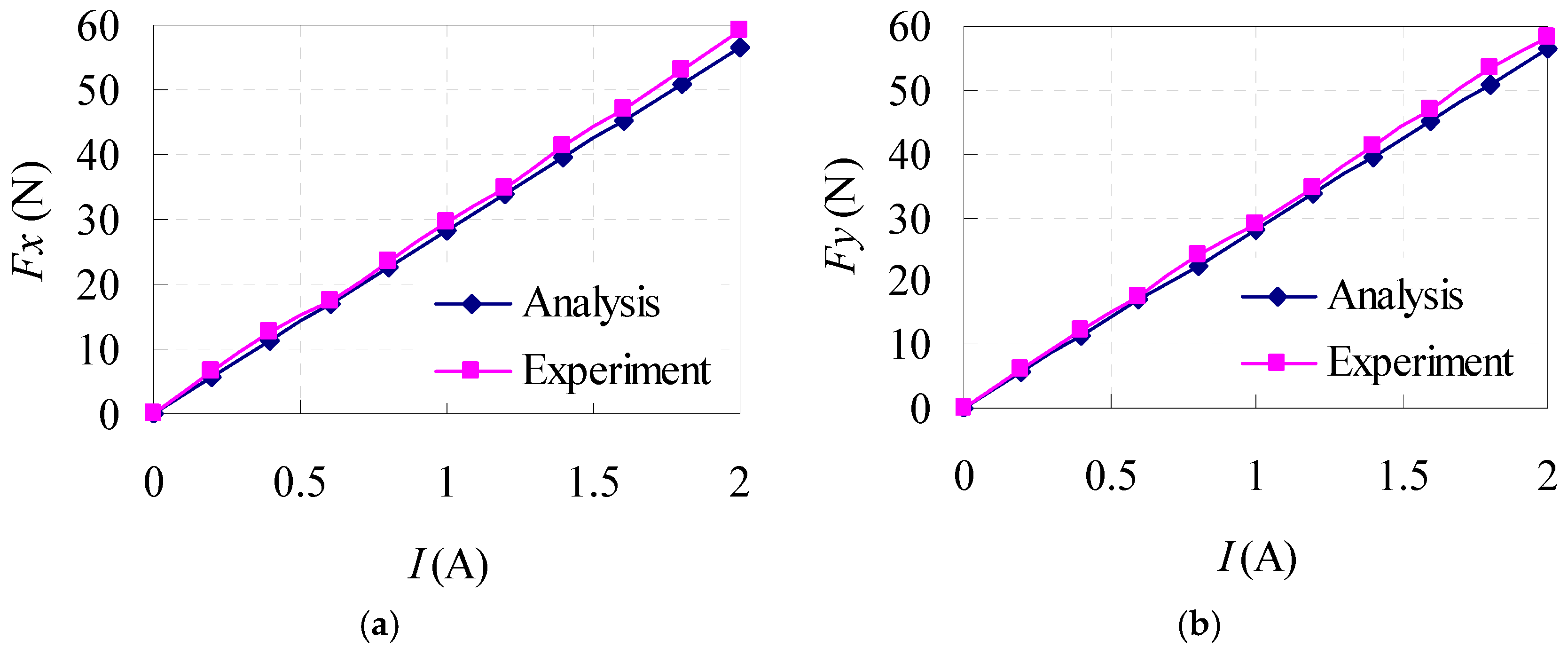
Figure 13 shows the force characteristics versus current. Both of the forces in the x and y directions increase linearly with the increase of the current. The measured forces agree well with the analytical model. Under the rated current I = 1.8 A, the measured forces in the x and y directions are 52.3 N and 52.9 N, respectively. The corresponding force coefficients are 29.06 N/A and 29.39 N/A, respectively. The force coefficient difference due to the directions is only 1.1%. Therefore, the force characteristics of the proposed planar motor reflect a good symmetry in the x and y directions.
5. Conclusions
In this study, a short-stroke Lorentz-force-driven planar motor was researched. We analyzed the working principle and built the analytical model of the planar motor based on the equivalent magnetic charge and image method. Then, the analytical force expression of the planar motor was derived. Additionally, the design optimization according to different design emphasis were conducted. Based on the derived expressions of the force, force density, and acceleration, the corresponding characteristics curves versus two main parameters were obtained. According to the results, some optimization references for this type of planar motor can be drawn as follows:
- Based on a certain height and pole pitch for the planar motor, the force reaches its maximum value when the ratio between the permanent thickness and the total air-gap length is around 0.5 (i.e., γ = 0.5).
- The force density first increases and then decreases with the increase of parameter γ when parameter λ is constant, but the acceleration will gradually decrease. On the contrary, the acceleration first increases and then decreases with the increase of parameter λ when parameter γ is constant, but the force density will gradually increase. Therefore, the reasonable value range for the parameter γ is between 0.4 and 0.6 to balance the force, the force density, and the acceleration. A larger value of parameter γ will cause the decrease of force density and acceleration, but a smaller value of parameter γ will cause the decrease of force.
Finally, a prototype of the planar motor was manufactured and tested. The electric parameters and the forces both in the x and y directions were obtained. The experimental results showed good agreement with the analytical model. Further research will focus on the temperature rise inhibition, dynamic performance analysis, and lightweight design.
Acknowledgments
The work described in this paper is supported by the Special Financial Grant from China Postdoctoral Science Foundation (2016T90286), the General Financial Grant from China Postdoctoral Science Foundation (2015M581444), and Special Financial Grant from Heilongjiang Postdoctoral Science Foundation (LBH-TZ0601).
Author Contributions
He Zhang contributed to the organization of the research work, including the modeling, design optimization, and manuscript preparation. Baoquan Kou contributed to the experiments and data analysis.
Conflicts of Interest
The authors declare no conflict of interest.
References
- Kou, B.Q.; Zhang, H.; Li, L.Y. Analysis and design of a novel 3-DOF Lorentz-force-driven DC planar motor. IEEE Trans. Magn. 2011, 47, 2118–2126. [Google Scholar]
- Kuo, S.K.; Menq, C.H. Modeling and control of a six-axis precision motion control stage. IEEE/ASME Trans. Mechatron. 2005, 10, 50–59. [Google Scholar] [CrossRef]
- Verma, S.; Kim, W.J.; Gu, J. Six-axis nanopositioning device with precision magnetic levitation technology. IEEE/ASME Trans. Mechatron. 2004, 9, 384–391. [Google Scholar] [CrossRef]
- Zhang, Z.P.; Menq, C.H. Six-axis magnetic levitation and motion control. IEEE/ASME Trans. Robot. 2007, 23, 196–205. [Google Scholar] [CrossRef]
- Dejima, S.; Gao, W.; Shimizu, H.; Kiyono, S.; Tomita, Y. Precision positioning of a five degree-of-freedom planar motion stage. Mechatronics 2005, 15, 969–987. [Google Scholar] [CrossRef]
- Holmesa, M.; Hockena, R.; Trumperb, D. The long-range scanning stage: A novel platform for scanned-probe microscopy. Precis. Eng. 2000, 24, 191–209. [Google Scholar] [CrossRef]
- Snitka, V. Ultrasonic actuators for nanometer positioning. Ultrasonics 2000, 38, 20–25. [Google Scholar] [CrossRef]
- Chu, X.C.; Wang, J.W.; Yuan, S.M.; Li, L.T.; Cui, H.C. A screw-thread-type ultrasonic actuator based on a langevin piezoelectric vibrator. Rev. Sci. Instrum. 2014, 85, 065002. [Google Scholar] [CrossRef] [PubMed]
- Liu, Y.X.; Chen, W.S.; Feng, P.L.; Liu, J.K. A linear piezoelectric actuator using the first-order bending modes. Ceram. Int. 2013, 39, S681–S684. [Google Scholar] [CrossRef]
- Chen, M.Y.; Wang, M.J.; Fu, L.C. Dual-axis maglev guiding system modeling and controller design for wafer transportation. In Proceedings of the Conference on Decision & Control, Phoenix, AZ, USA, 7–10 December 1999.
- Chen, M.Y.; Wang, M.J.; Fu, L.C. A novel dual-axis repulsive maglev guiding system with permanent magnet: Modeling and controller design. IEEE/ASME Trans. Mechatron. 2003, 8, 77–86. [Google Scholar] [CrossRef]
- Sawyer, B.A. Magnetic Positioning Device. US Patent 3,376,578, 22 July 1968. [Google Scholar]
- Pelta, E.R. Two-axis sawyer motor for motion systems. IEEE Control Syst. Mag. 1987, 7, 20–24. [Google Scholar] [CrossRef]
- Pan, J.F.; Cheung, N.C.; Gan, W.C.; Zhao, S.W. A novel planar switched reluctance motor for industrial applications. IEEE Trans. Magn. 2006, 42, 2836–2839. [Google Scholar] [CrossRef]
- Pan, J.F.; Cheung, N.C.; Yang, J. High-precision position control of a novel planar switched reluctance motor. IEEE Trans. Ind. Electron. 2005, 52, 1644–1652. [Google Scholar] [CrossRef]
- Fujii, N.; Fujitake, M. Two-dimensional drive characteristics by circular-shaped motor. IEEE Trans. Ind. Electron. 1999, 35, 803–809. [Google Scholar] [CrossRef]
- Kim, W.J.; Trumper, D.L. High-precision magnetic levitation stage for photolithography. Precis. Eng. 1998, 22, 66–77. [Google Scholar] [CrossRef]
- Cho, H.S.; Jung, H.K. Analysis and design of synchronous permanent-magnet planar motors. IEEE Trans. Energy Convers. 2002, 17, 492–499. [Google Scholar] [CrossRef]
- Jansen, J.W.; van Lierop, C.M.M.; Lomonova, E.A.; Vandenput, A.J.A. Modeling of magnetically levitated planar actuators with moving magnets. IEEE Trans. Magn. 2007, 43, 15–25. [Google Scholar] [CrossRef]
- Lei, J.; Luo, X.; Chen, X.; Yan, T. Modeling and analysis of a 3-DOF Lorentz-force-driven planar motion stage for nanopositioning. Mechatronics 2010, 20, 553–565. [Google Scholar] [CrossRef]
- Kim, W.J.; Verma, S.; Shakir, H. Design and precision construction of novel magnetic-levitation-based multi-axis nanoscale positioning systems. Precis. Eng. 2007, 31, 337–350. [Google Scholar] [CrossRef]
- Zhang, H.; Kou, B.Q.; Zhang, H.L.; Jin, Y.X. A three-degree-of-freedom short-stroke Lorentz-force-driven planar motor using a Halbach permanent-magnet array with unequal thickness. IEEE Trans. Ind. Electron. 2015, 62, 3640–3650. [Google Scholar] [CrossRef]
- Choi, Y.M.; Gweon, D.G. A high-precision dual-servo stage using Halbach linear active magnetic bearings. IEEE/ASME Trans. Mechatron. 2011, 16, 925–931. [Google Scholar] [CrossRef]
- Chen, M.Y.; Lin, T.B.; Huang, S.K.; Fu, L.C. Design and experiment of a macro-micro planar maglev positioning system. IEEE Trans. Ind. Electron. 2012, 59, 4128–4139. [Google Scholar] [CrossRef]
- Ravaud, R.; Lemarquand, G.; Lemarquand, V.; Depollier, C. Analytical calculation of the magnetic field created by permanent magnet rings. IEEE Trans. Magn. 2008, 44, 1982–1989. [Google Scholar] [CrossRef]
- Ravaud, R.; Lemarquand, G.; Lemarquand, V.; Depollier, C. Permanent magnet couplings: Field and torque three-dimensional expressions based on the coulombian model. IEEE Trans. Magn. 2009, 45, 1950–1958. [Google Scholar] [CrossRef]
Figure 1.
Basic configuration of the Lorentz-force-driven planar motor.
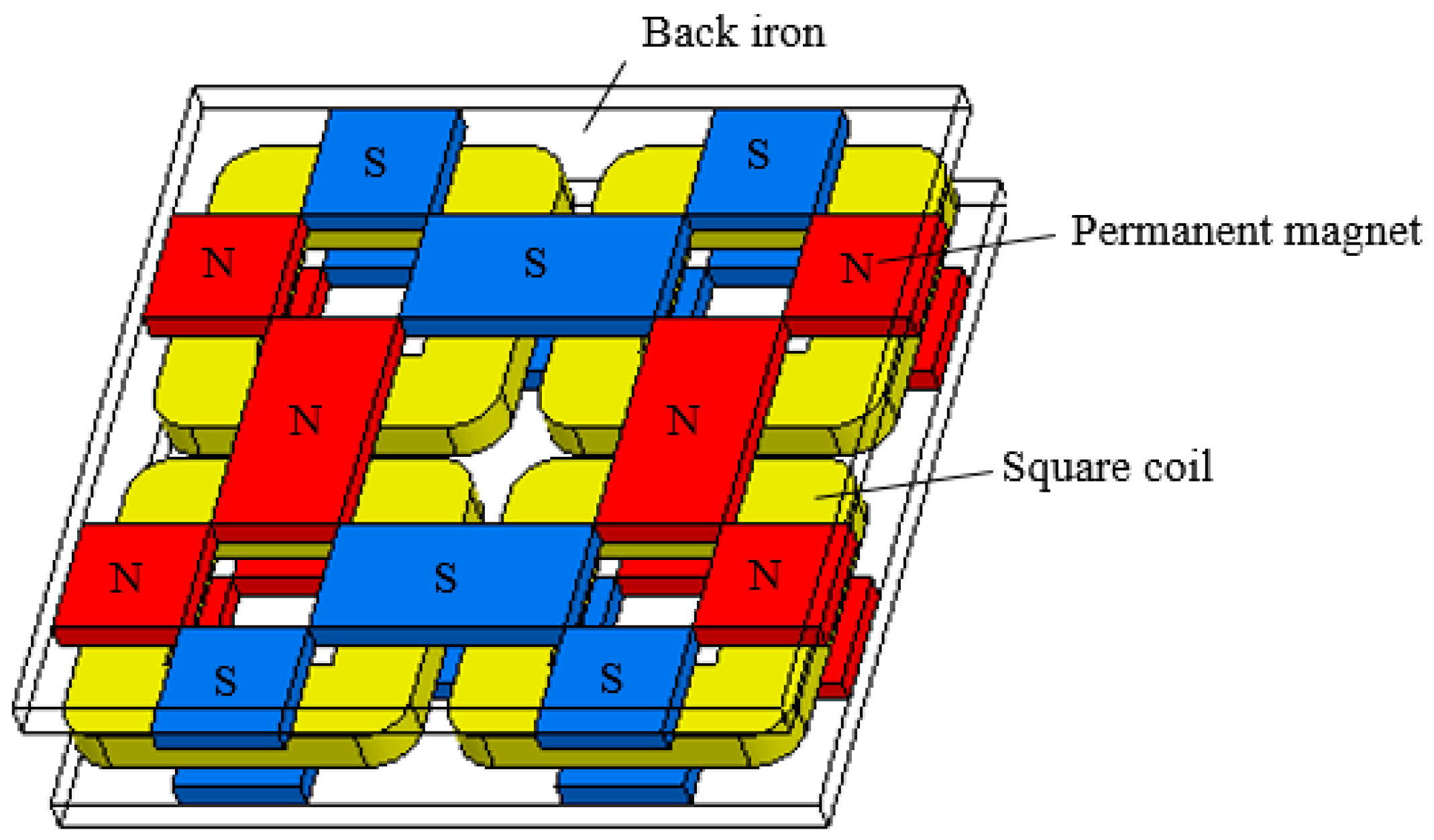
Figure 2.
Lorentz-force-driven unit. (PM: Permanent Magnet).

Figure 3.
Working principle of the Lorentz-force-driven planar motor: (a) Moving in the x axis; (b) Moving in the y axis; (c) Rotating about the z axis.
Figure 3.
Working principle of the Lorentz-force-driven planar motor: (a) Moving in the x axis; (b) Moving in the y axis; (c) Rotating about the z axis.

Figure 4.
Coordinate system.

Figure 5.
Side view of one coil and its relating permanent magnets.
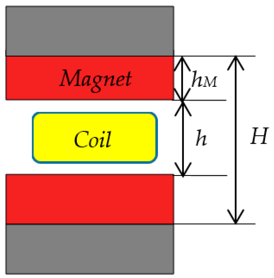
Figure 6.
Force characteristic versus parameter γ: (a) with different H when τ = 50 mm; (b) with different τ when H = 20 mm.
Figure 6.
Force characteristic versus parameter γ: (a) with different H when τ = 50 mm; (b) with different τ when H = 20 mm.
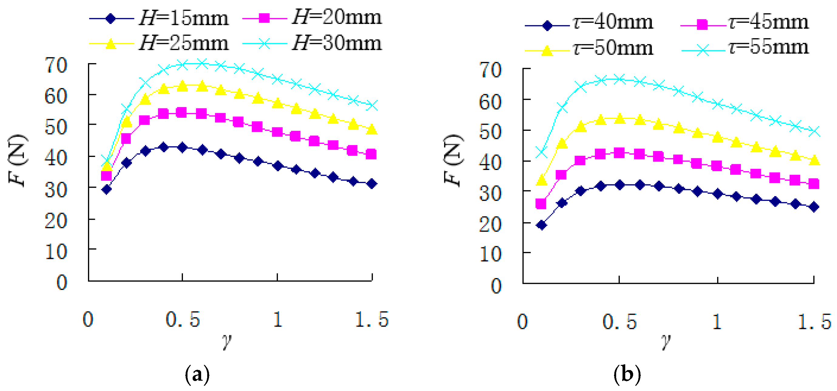
Figure 7.
Top and side view of the planar motor.
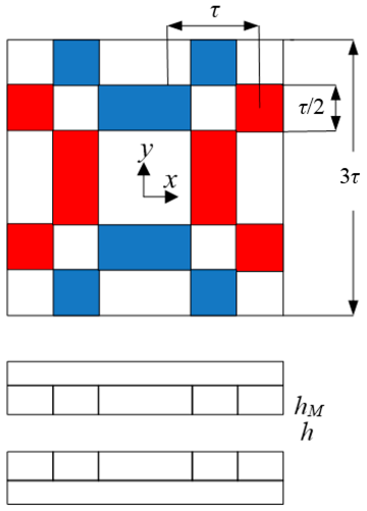
Figure 8.
Force characteristic versus parameters γ and λ: (a) with different λ; (b) with different γ.
Figure 8.
Force characteristic versus parameters γ and λ: (a) with different λ; (b) with different γ.
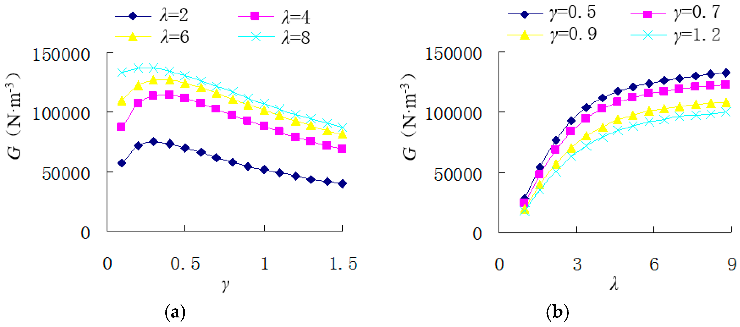
Figure 9.
Acceleration versus parameters γ and λ: (a) with different λ; (b) with different γ.

Figure 10.
Model and prototype of the square coil: (a) model and sizes; (b) actual square coil.
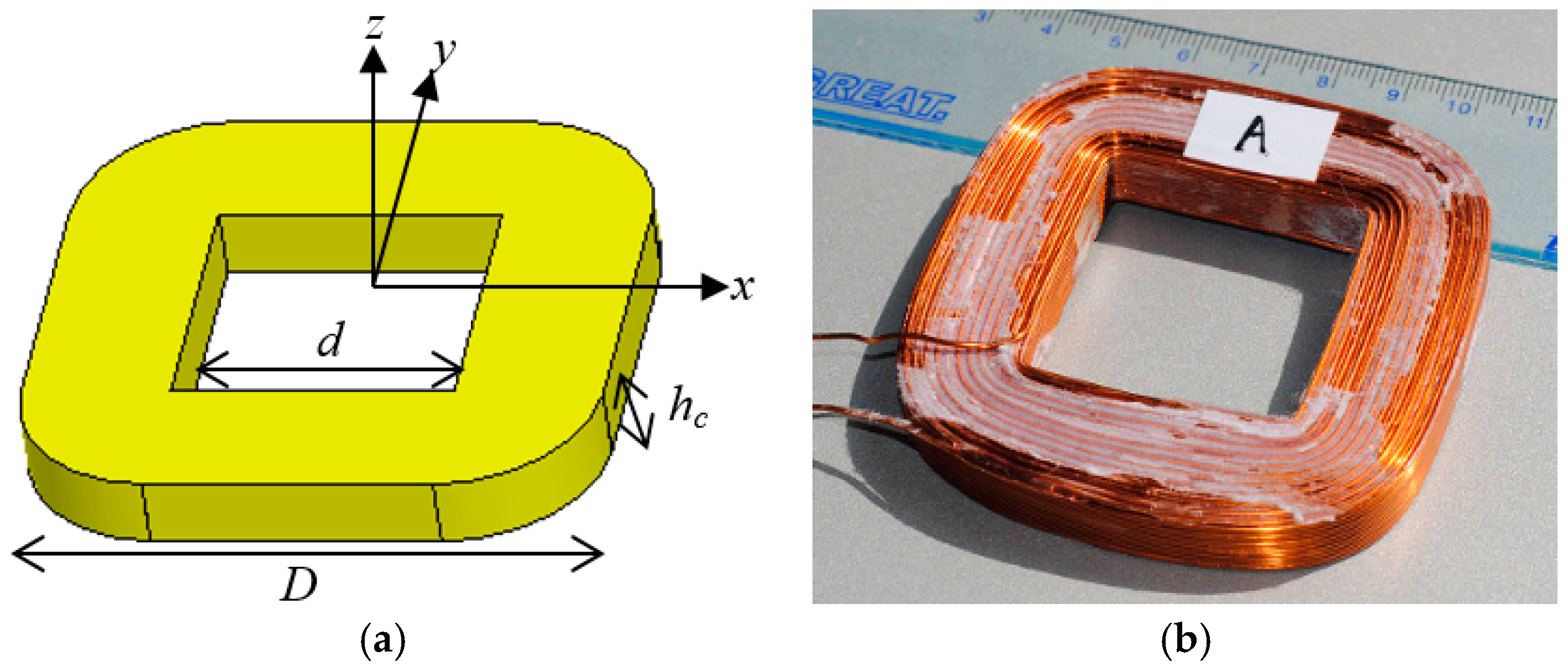
Figure 11.
Inductance calculation model for the square coil.
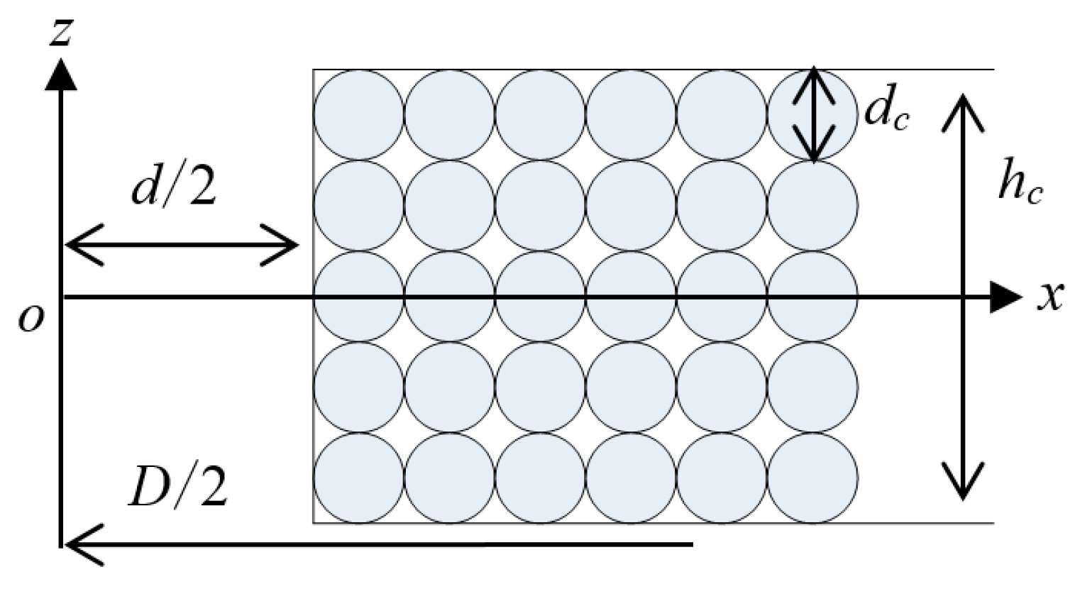
Figure 12.
Planar motor force experimental system. (DC: Direct Current).
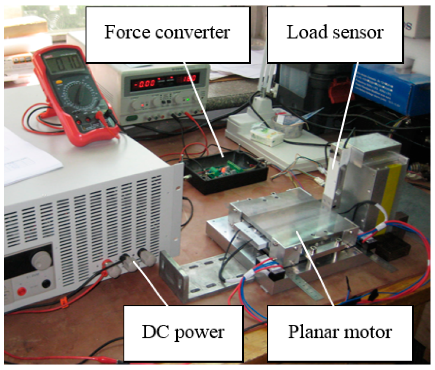
Figure 13.
Force characteristics versus current: (a) force in the x direction; (b) force in the y direction.
Figure 13.
Force characteristics versus current: (a) force in the x direction; (b) force in the y direction.

| Item | Symbol | Value | Unit |
|---|---|---|---|
| inner width | d | 35.76 | mm |
| outer width | D | 71.28 | mm |
| thickness | hc | 9.60 | mm |
| wire diameter | dc | 0.76 | mm |
| conductor diameter | dc1 | 0.71 | mm |
| number of turns | N | 276 | - |
| Coil | Value | Unit |
|---|---|---|
| A | 2.341 | Ω |
| B | 2.348 | Ω |
| C | 2.350 | Ω |
| D | 2.349 | Ω |
| Coil | Value | Unit |
|---|---|---|
| A | 4.593 | mH |
| B | 4.595 | mH |
| C | 4.592 | mH |
| D | 4.572 | mH |
| Item | Symbol | Value | Unit |
|---|---|---|---|
| Magnet type | - | N38 | - |
| Magnet thickness | hM | 5.5 | mm |
| Pole pitch | τ | 54 | mm |
| Total air-gap length | h | 13 | mm |
| Main coefficient 1 | λ | 4.15 | - |
| Main coefficient 2 | γ | 0.42 | - |
| Pole-arc coefficient | αi | 0.515 | - |
© 2016 by the authors; licensee MDPI, Basel, Switzerland. This article is an open access article distributed under the terms and conditions of the Creative Commons Attribution (CC-BY) license (http://creativecommons.org/licenses/by/4.0/).
Share and Cite
MDPI and ACS Style
Zhang, H.; Kou, B. Design and Optimization of a Lorentz-Force-Driven Planar Motor. Appl. Sci. 2017, 7, 7. https://doi.org/10.3390/app7010007
AMA Style
Zhang H, Kou B. Design and Optimization of a Lorentz-Force-Driven Planar Motor. Applied Sciences. 2017; 7(1):7. https://doi.org/10.3390/app7010007
Chicago/Turabian StyleZhang, He, and Baoquan Kou. 2017. "Design and Optimization of a Lorentz-Force-Driven Planar Motor" Applied Sciences 7, no. 1: 7. https://doi.org/10.3390/app7010007
Note that from the first issue of 2016, this journal uses article numbers instead of page numbers. See further details here.