Wind-Induced Fatigue Analysis of High-Rise Steel Structures Using Equivalent Structural Stress Method

Abstract

Welded beam-to-column connections of high-rise steel structures are susceptive to fatigue damage under wind loading. However, most fatigue assessments in the field of civil engineering are mainly based on nominal stress or hot spot stress theories, which has the disadvantage of dependence on the meshing styles and massive curves selected. To address this problem, in this paper, the equivalent structural stress method with advantages of mesh-insensitive quality and capability of unifying different stress-life curves (S-N curves) into one is introduced to the wind-induced fatigue assessment of a large-scale complicated high-rise steel structure. The multi-scale finite element model is established and the corresponding wind loading is simulated. Fatigue life assessments using equivalent structural stress method, hot spot stress method and nominal stress method are performed, and the results are verified and comparisons are made. The mesh-insensitive quality is also verified. The results show that the lateral weld toe of the butt weld connecting the beam flange plate and the column is the location where fatigue damage most likely happens. Nominal stress method considers fatigue assessment of welds in a more global way by averaging all the stress on the weld section while in equivalent structural stress method and hot spot method local stress concentration can be taken into account more precisely.

1. Introduction

Wind loading is a major loading to high-rise structures, which not only causes vibration but may bring about fatigue problems as well, for the fluctuating wind as a random loading can be regarded as a sort of cycle loading for high-rise structures and may cause fatigue crack initiation in components where large stress concentration exists and finally leads to fatigue failure. Several cases of wind-induced fatigue failure of steel mast structures have been found in history [1]. As to high-rise steel frame structures whose beam-to-column connections are mostly welded and local stress concentration inevitably exists, fatigue cracks are prone to initiate near welded joints in beam-to-column connections, which certainly brings potential danger of fatigue failure.

At present, fatigue life assessments in the field of civil engineering are mainly based on nominal stress or hot spot stress theories. For example, Repetto [2,3,4] selected several types of mast structures, including telegraph poles and lamp-posts, and, by considering the changing wind speed and wind direction simultaneously, performed fatigue assessment of along-wind and crosswind response effect on structures from the frequency domain and time domain, respectively. Jia [5,6] presented a practical and efficient approach for calculating wind-induced fatigue of tubular structures and studied the effects of the wind direction and wind grid size on the high cycle fatigue of the structure. However, the fatigue assessment of welded joints based on nominal stress and hot spot stress methods cannot accurately consider the effect of the notch effect, which is a strong stress concentration near notch roots or notch toes. As a result, many new methods and concepts based on local stress have been introduced into practical engineering structures. Righiniotis [7] used the theory of critical distances (TCD) to perform fatigue analysis of a riveted railway bridge by a global–local FE (Finite element) model. Sonsino [8] applied notch stress concept for several engineering structures including MAG-welded offshore K-nodes, sandwich panels for ship decks, spot-welded automotive doors and MAG-welded automotive trailing links.

However, the drawbacks of the methods stated above are very clear. In nominal stress, joints are classified into various joint types and each type owns a design S-N curve, which inevitably confuse engineers when selecting the accurate curve, while in hot spot stress and local stress, the results are largely dependent on the meshing style, which will bring high requirement of meshing density and thus exhaust massive computing resources and time, especially in large scale complex structures. Therefore, the desire to establish a mesh-insensitive method capable of unifying various curves into one single curve has received considerable attention. The equivalent structural stress method is the ideal combination of these two advantages.

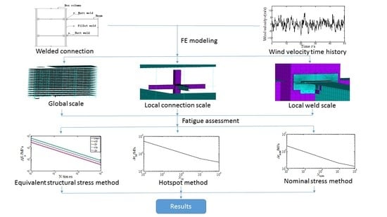
In this paper, the equivalent structural stress method is introduced into the fatigue life assessment of a typical high-rise steel braced frame structure. A multi-scale FE model is established and the corresponding wind simulation is performed. The fatigue life of the welded beam-to-column connection is assessed based on equivalent structural stress method, hot spot method and nominal stress method and comparisons are made.

2. Equivalent Structural Stress Method

The equivalent structural stress method was first proposed by Dong [9], who defined the structural stress $\left({\mathsf{\sigma }}_s\right)$ to be the superposition of a membrane component (${\mathsf{\sigma }}_m$) and a bending component (${\mathsf{\sigma }}_b$):

$${\mathsf{\sigma }}_s={\mathsf{\sigma }}_m+{\mathsf{\sigma }}_b$$

(1)

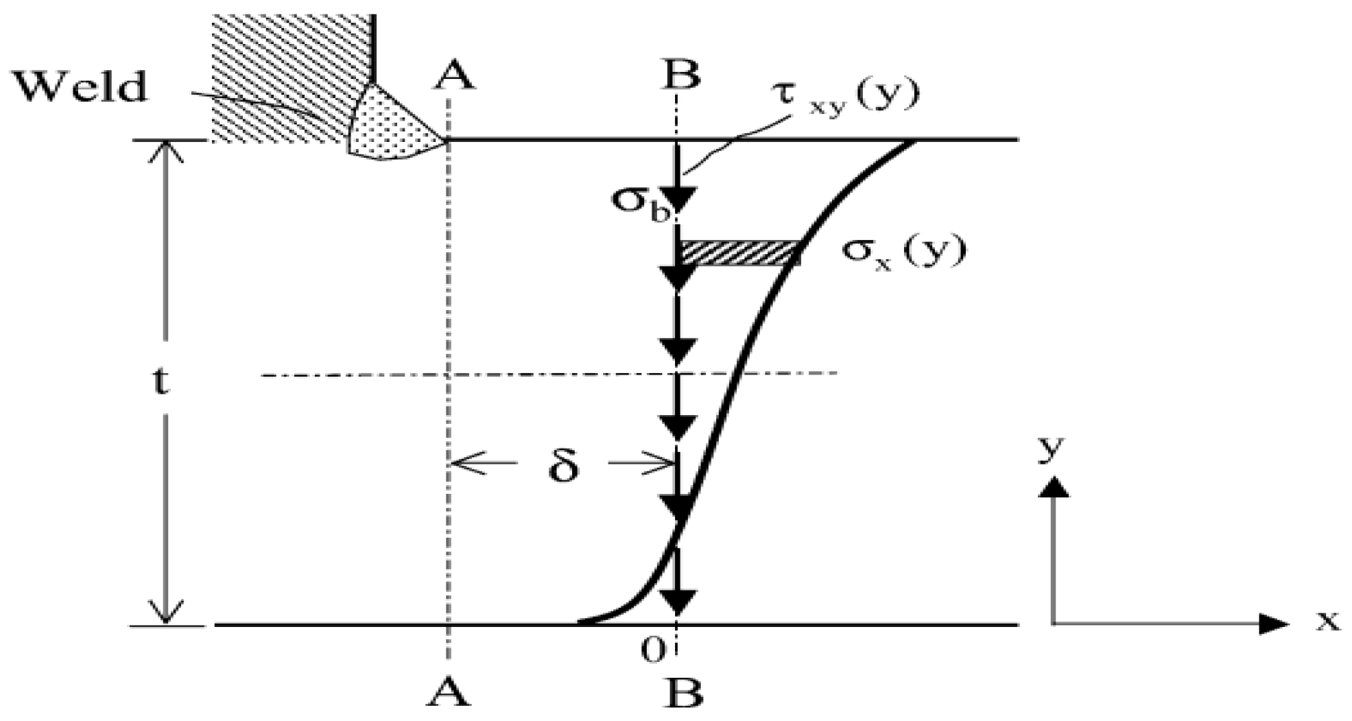
A typical T-fillet weld toe is illustrated in Figure 1, the stress distribution through the thickness at the weld toe is assumed to be monotonic with the peak stress occurring at the weld toe. Two reference sections are defined, Section A–A, where the normal structural stress (${\mathsf{\sigma }}_s$) is defined at the weld toe, and Section B–B, where a row of elements with same length of $\mathsf{\delta }$ which represents the distance between Sections A–A and B–B at the weld toe can be used in the FE model so both local normal stress ${\mathsf{\sigma }}_x\left(y\right)$ and shear stress ${\mathsf{\tau }}_{xy}\left(y\right)$ can be directly obtained from a FE solution. The plate thickness is t and the transverse shear of the structural stress components is ignored. The local coordinate is established as in Figure 1. By imposing equilibrium conditions that the force balances in x direction evaluated along B–B and moment balances in Section A–A at y = 0 between Sections A–A and B–B, the structural stress components ${\mathsf{\sigma }}_m$ and ${\mathsf{\sigma }}_b$ must satisfy the following conditions:

$${\mathsf{\sigma }}_m=\frac{1}{t}{{\displaystyle \int }}_0^t{\mathsf{\sigma }}_x\left(y\right)dy$$

(2)

$${\mathsf{\sigma }}_m·\frac{t^2}{2}+{\mathsf{\sigma }}_b·\frac{t^2}{6}={{\displaystyle \int }}_0^t{\mathsf{\sigma }}_x\left(y\right)ydy+\mathsf{\delta }{{\displaystyle \int }}_0^t{\mathsf{\tau }}_{xy}\left(y\right)dy$$

(3)

It is clear that if element size ($\mathsf{\delta }$) is small or transverse, shear, which is one of the integral terms on the right-hand side of Equation (3), is negligible, and the integral representations of ${\mathsf{\sigma }}_b$ and ${\mathsf{\sigma }}_m$ in Equations (2) and (3) can be directly evaluated at Section A–A in Figure 1.

In hot spot stress or other local stress analysis, the stress values within some distance from the weld toe can change significantly with the changing meshing style while in the equivalent structural stress analysis the stress deduced from elementary structural mechanics theory will be less affected by the meshing style, so the first advantage of mesh-insensitive is achieved. By the effects of stress concentration, thickness of plates and loading on the fatigue life of welds being considered, and based on thousands of fatigue test data, the welded joint fatigue S-N curves based on the nominal stress are compressed into a single master S-N curve based on the equivalent structural stress which can be deduced from the structural stress ${\mathsf{\sigma }}_s$ above. As a result, the second advantage of unifying different curves is realized.

This method has been applied to fatigue assessment of several types of welded joints including butt welds, fillet welds and spot welds and good correlation is proven [10,11]. Later, Dong extended this method to medium and low cycle fatigue assessment, by defining a structural strain parameter [12]. However, the appliance of this method to real three-dimensional complex structure is still tricky because, in three-dimensional circumstances, the formulae are a little different from Equations (2) and (3) and need modification. Besides, in a large scale structure, acquiring detailed stress time-history near welds needs multi-scale modeling technique, which is not an easy task.

3. High-Rise Steel Braced Frame Structure

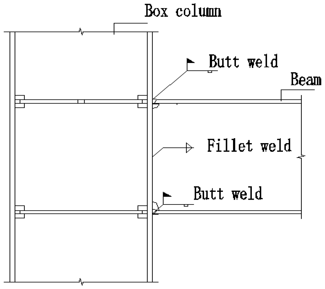
A typical high-rise steel braced frame structure is chosen, which is located in a downtown area of a medium city in China, with the plane shape to be a regular rectangular. The plane length is 70.65 m and the width is 22.6 m. The building height is 71.6 m with 17 floors above the ground level and a one-floor basement underground. The steel used in this structure has Poisson’s ratio 0.3 and elastic modulus 206 GPa. The box-section columns underground are steel reinforced concrete columns and those above ground level are pure steel columns. The column sections change from 600 mm × 600 mm× 32 mm to 500 mm × 500 mm × 24 mm with the increase of height. The section of braces is mainly H-shape, which is 350 mm × 300 mm × 18 mm × 24 mm, supported by BRB. The beams are hot-rolled H-beams which are connected to columns by welded joints, as shown in Figure 2, where the two beam flange plates are connected by butt welds and the web plate is connected by fillet welds.

4. Wind Simulation

In simplicity, it is assumed that the wind direction is constant and always perpendicular to the structural lateral surface and only along-wind response is taken into account. Since this building is in China, the selection of design basic wind speed refers to Chinese specifications. Actually, if other specifications are selected, the corresponding design basic wind speed can be transformed from that in Chinese specifications by converting the standard height, terrain roughness, etc. The fatigue assessment procedure stated in this paper keeps the same. According to Chinese specifications [13], in this city, when the terrain roughness is defined as Area B, which means the outskirts area of the city, return period is 100 years, standard height is 10 m and average time interval is 10 min, the standard mean wind pressure is $p_0=0.45\mathrm{kPa}$ and the mean wind speed can be calculated as $v_0=\sqrt{1600p_0}=26.83\mathrm{m}/\mathrm{s}$. Since this structure is located in a downtown area (the terrain roughness is defined as Area C which means the downtown area with intensive buildings nearby), the mean wind speed is transformed into $v_{a0}=20.23\mathrm{m}/\mathrm{s}$. The mean wind speed profile takes the form of a power law as:

$$U\left(z\right)=U_0{\left(\frac{z}{z_0}\right)}^{\mathsf{\alpha }}$$

(4)

where z₀ is the reference height which is taken as 10 m; U₀ is the wind speed at the reference height; which is taken as $20.23\mathrm{m}/\mathrm{s}$ as stated above; and α is the exponent of the velocity profile, which is 0.22 for this case.

The harmonic superposition method is used to generate the random fluctuating wind time series, and Davenport spectrum is adopted as the power spectrum of velocity fluctuation [14], as shown in Equations (5) and (6):

$$\frac{n{S}_v\left(n\right)}{{\overline{v}}_{10}^2}=\frac{4k{x}^2}{n{\left(1+x^2\right)}^{\raisebox{1ex}{$3$}\!\left/ \!\raisebox{-1ex}{$4$}\right.}}$$

(5)

$$x=1200\frac{n}{{\overline{v}}_{10}}$$

(6)

where ${\overline{v}}_{10}$ is the mean wind speed in the standard height of 10 m, which is taken as $20.23\mathrm{m}/\mathrm{s}$ as stated above; n is the frequency of the fluctuating wind; k is the terrain roughness factor of this area, which is 0.03; and $S_v\left(n\right)$ is the power spectrum of velocity fluctuation.

Due to the large height and width of the high-rise structure, the horizontal and vertical spatial coherence of velocity fluctuation needs to be taken into consideration simultaneously, the square root of the coherence function $Coh\left(d,n\right)$ is as shown in Equations (7) and (8):

$$Coh\left(d,n\right)=\frac{S_{u_1{u}_2}\left(d,n\right)}{\sqrt{S_{u_1}\left(l,n\right)S_{u_2}\left(k,n\right)}}=e^{-c}$$

(7)

$$c=\frac{n{\left[c_x{\left(x-x^{\prime }\right)}^2+c_z{\left(z-z^{\prime }\right)}^2\right]}^{\frac{1}{2}}}{\frac{1}{2}\left[\overline{v}\left(z\right)+\overline{v}\left(z^{\prime }\right)\right]}$$

(8)

where l and k are two points on the structural surface and their coordinates are (x, z) and (x’, z′), respectively; the distance between them is d; $S_{u_1{u}_2}\left(d,n\right)$ is the cross spectrum; $S_{u_1}\left(l,n\right)$ and $S_{u_2}\left(k,n\right)$ are the self-power spectrum of these two points; $\overline{v}\left(z\right)$and $\overline{v}\left(z^{\prime }\right)$ are the mean wind speed in the height of z and z′; and c_z and c_x are constants, 10 and 16, respectively.

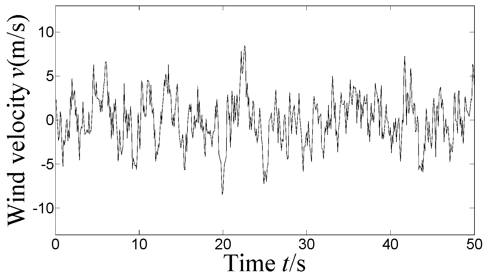
Because of the large computing amount involved in harmonic superposition method, during the generation of wind field it is not realistic to consider the horizontal and vertical spatial coherence of each beam-to-column connection. Therefore, in order to simplify the procedure, a total of 17 height reference points located at the height of each layer are selected in the vertical direction, and in the horizontal direction along the width, three reference points in each layer is selected every 35 m. Thus, a total of 51 wind time series are generated, whose duration is 50 s and the time interval is 0.1 s. Figure 3 is a typical fluctuating wind time-history obtained.

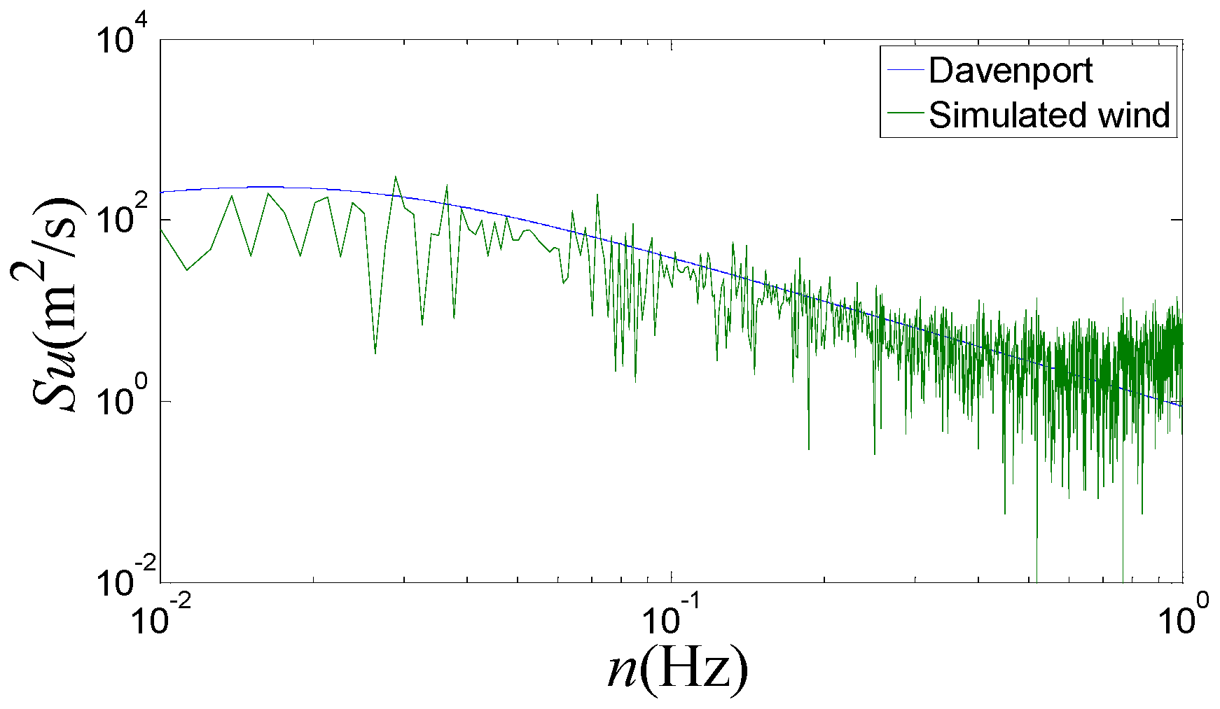
The obtained wind speed time-history is converted to power spectral density by inverse Fourier transform and is compared with the target Davenport spectrum. As shown in Figure 4, the smooth curve is the power spectral density curve of the Davenport spectrum, and the rest curve is the power spectral density curve of the simulated wind speed and found to be in agreement with Davenport spectrum well in most frequency bands.

5. Multi-Scale Model

Multi-scale modeling is a numerical modeling technique involved in FE modeling, which refers to the combined modeling of different scales. In multi-scale modeling, the important parts are modeled with relatively fine mesh while the parts which do not need attention are modeled with relatively coarse mesh. By appropriate connections at the boundaries of different element models, the force balance and deformation coordination are realized, thus more accurate results will be obtained by spending less computing resources and time.

In the structure, the beam-to-column connections in the ground floor are relatively easy to produce stress concentration, because the horizontal wind force and the gravity of the structure finally transmit to the ground floor through beams and columns. Since wind loading is much smaller than the gravity, under the gravity, in a beam-to-column connection the upper beam flange is easy to produce tension while the lower flange is easy to produce pressure, and as known to us all, when it comes to fatigue damage prevention, pressure is more conductive to the structure than tension. Thus, the upper flange is the position where fatigue cracks are easier to initiate and the welds connecting upper beam flange and the column is where local model is required.

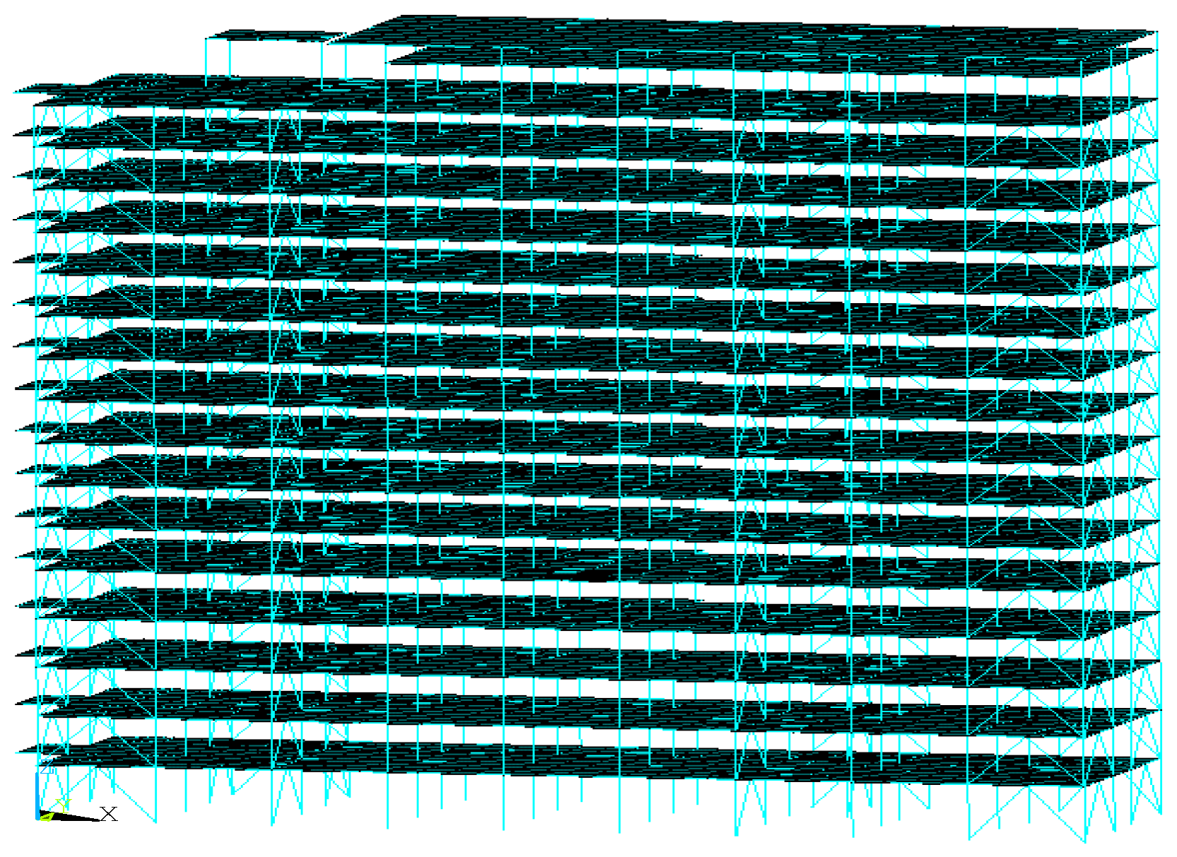
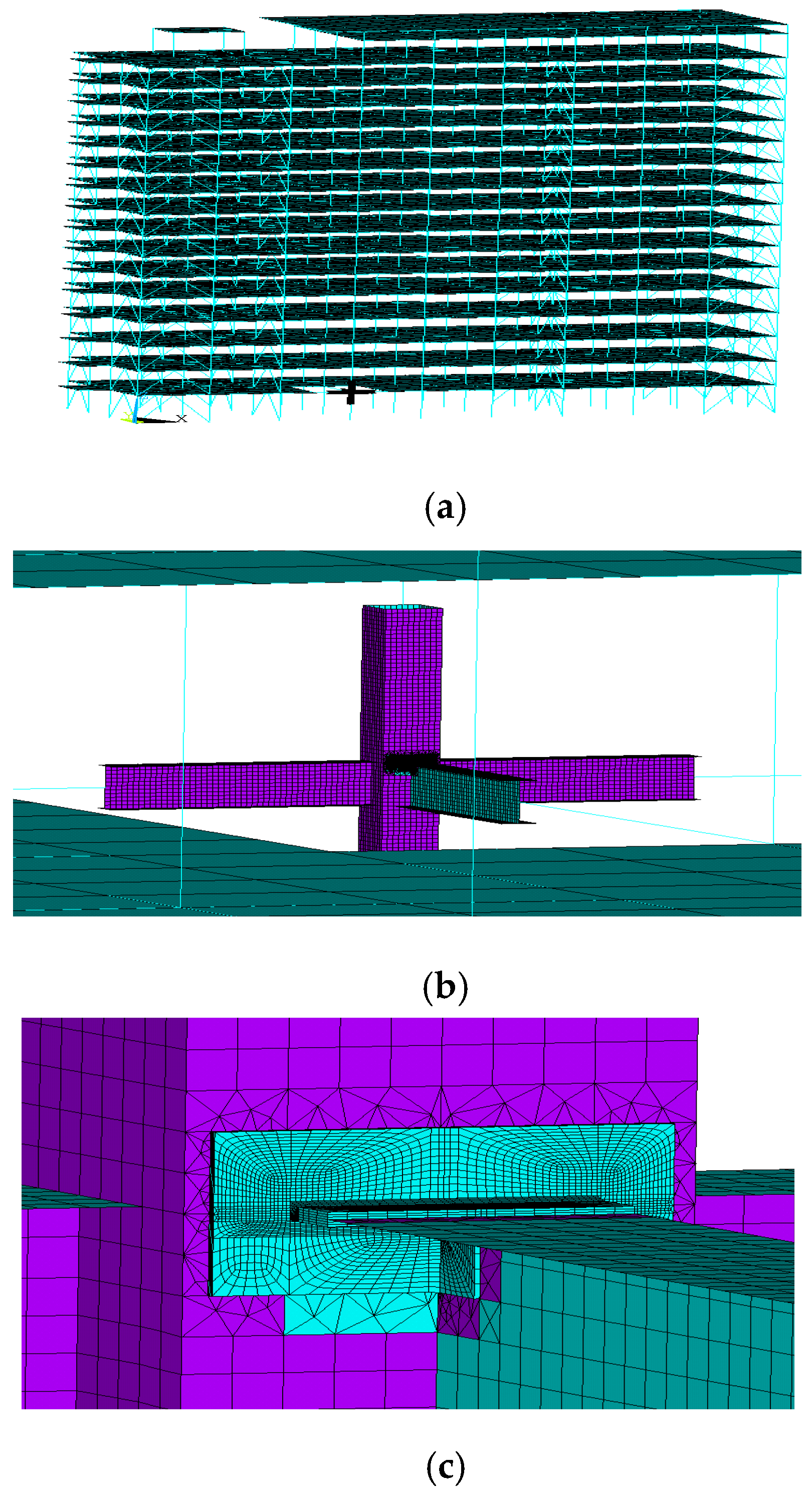
Thus, a multi-scale FE model is established by the commercial FE software ANSYS (ANSYS, Inc., Canonsburg, PA, USA) with a global scale model, a local connection scale model and a local weld scale model. In the global scale model, a model of the whole structure is established and beams and columns are simulated by element BEAM188 and floors are simulated by element SHELL63, as shown in Figure 5a. A typical beam-to-column connection considered to be more stress-concentrated in the first floor is chosen to establish the local connection scale model, whose beam and column are simulated by element SHELL63, as illustrated in Figure 5b. The upper flange plate on the inner beam where the tension stress concentration usually happens is chosen to establish a local weld scale model, which is simulated by eight-node element SOLID45, as shown in Figure 5c. The connections among the three different scale models are created by establishing the rigid region which can provide the desirable constraint equation. Thus, the multi-scale element model embodies the force transition from the global scale to the local connection scale then to the local weld scale and the connection between beam elements to shell elements then to solid elements.

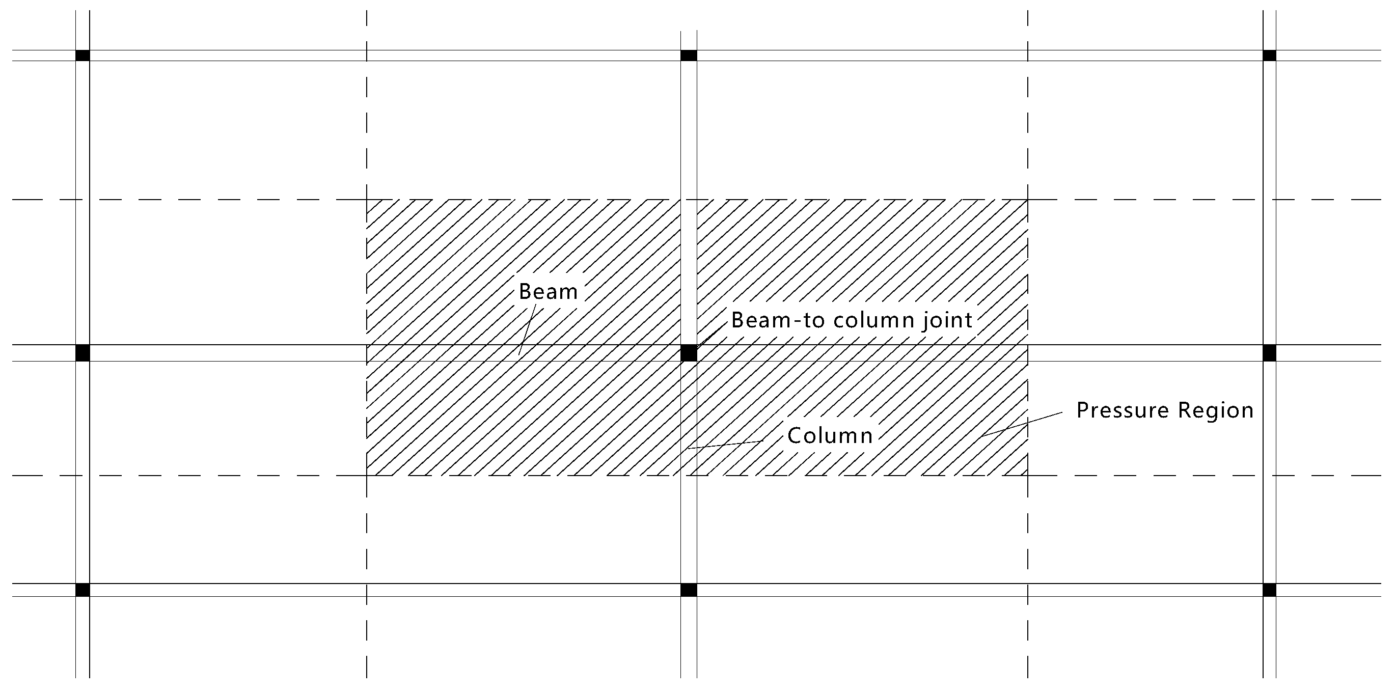
The structural windward surface is divided into several pressure regions, each of which contains a beam-to-column connection, as illustrated in Figure 6. The wind pressure on each pressure region can be approximately equivalent to a concentrated force in the region center, which is the exact location where each beam-to-column connection is, as represented in Figure 6 as the black dot in the pressure region center. Therefore, the simulated wind speed time history curves are transformed into corresponding wind loading (concentrated force) time history curves by Equation (9).

$$\begin{array}{ll}{P}_i=A_i{\mathsf{\mu }}_s{W}_i\left(z,t\right)& =\frac{1}{2}{A}_i{\mathsf{\mu }}_s\mathsf{\rho }{V_i}^2\left(z,t\right)=\frac{1}{2}{A}_i{\mathsf{\mu }}_s\mathsf{\rho }{\left[{\overline{\mathrm{v}}}_i\left(z\right)+v_i\left(z,t\right)\right]}^2\\ & =\frac{1}{2}{A}_i{\mathsf{\mu }}_s\mathsf{\rho }{{\overline{v}}_i}^2\left(z\right)+\frac{1}{2}{A}_i{\mathsf{\mu }}_s\mathsf{\rho }\left[2{\overline{v}}_i\left(z,t\right)+{v_i}^2\left(z,t\right)\right]\\ & \approx \frac{1}{2}{A}_i{\mathsf{\mu }}_s\mathsf{\rho }{{\overline{v}}_i}^2\left(z\right)+A_i{\mathsf{\mu }}_s\mathsf{\rho }{\overline{v}}_i\left(z\right)v_i\left(z,t\right)\end{array}$$

(9)

where $P_i$ is the concentrated force exerted on i-th beam-to-column connection; ${\overline{v}}_i\left(z\right)$, $v_i\left(z,t\right)$ and $V_i\left(z,t\right)$ are the mean wind speed, fluctuating wind speed and the natural wind speed of i-th beam-to-column connection and the natural wind speed is the sum of the mean wind speed and the fluctuating wind speed, respectively; $\mathsf{\rho }$ is the air density; A_i is the pressure region i-th beam-to-column connection belongs to, which is illustrated in Figure 6 as the shaded area; and ${\mathsf{\mu }}_s$ is the shape coefficient of the structure, and, for a rectangle, it is taken as 1.3 according to Chinese specifications.

By time-history analysis, the stress time-history curve near the connecting weld of the selected the beam-to-column connection can be obtained and thus the fatigue assessment can be performed.

6. Fatigue Assessment

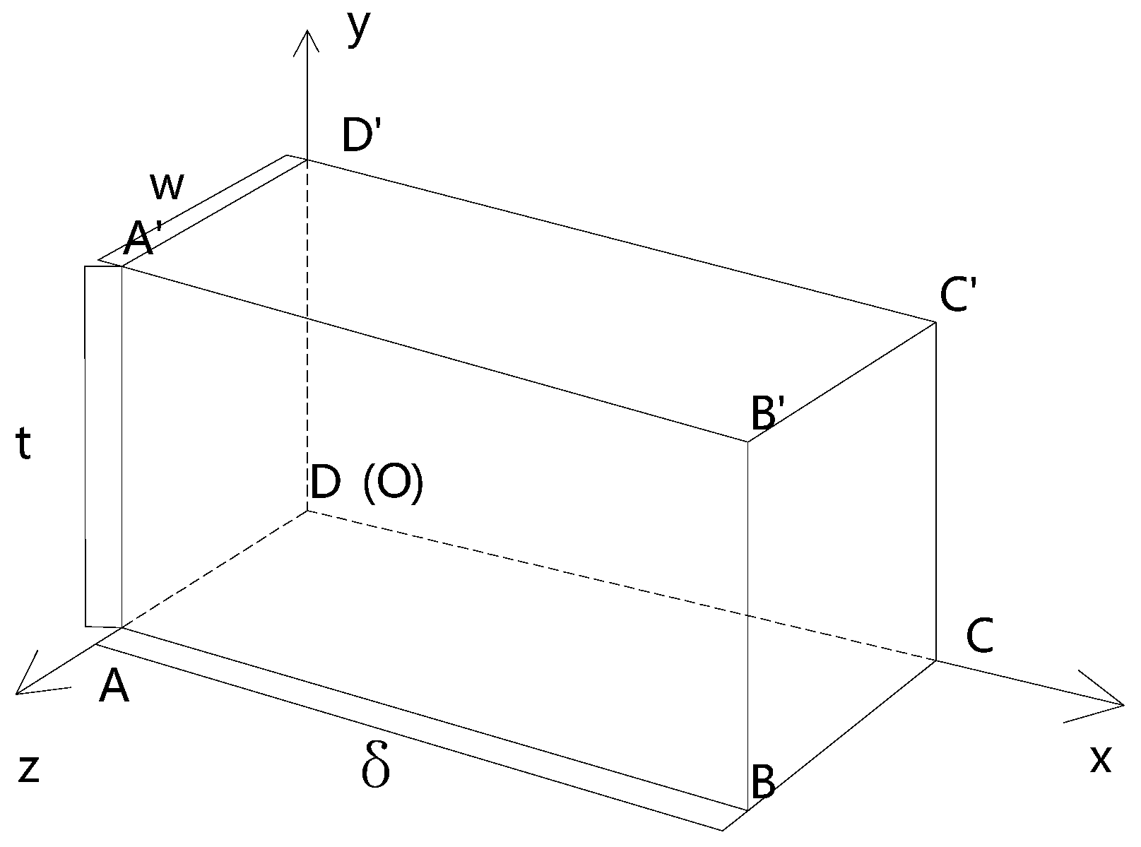
Regarding three-dimensional structures, due to the three-dimensional solid elements involved, a modification of the formulae stated above is necessary, which is mainly based on two dimensional planar circumstances. A three-dimensional isolated body is taken from the weld toe, where two reference sections are defined. They are AA’D’D along the thickness and BB’C’C defined $\mathsf{\delta }$ away from AA’D’D. A local coordinate is established as shown in Figure 7 and the origin O is defined at the bottom of AA’D’D. By the space effect being considered, the modified formulae can be obtained by imposing equilibrium conditions that the force balances in x direction evaluated along BB’C’C and moment balances at Point O, as shown in Equations (10) and (11). The membrane stress ${\mathsf{\sigma }}_{m3D}$ and bending stress ${\mathsf{\sigma }}_{b3D}$ can be got and the structural stress ${\mathsf{\sigma }}_{s3D}$ is obtained as Equation (12).

$${\mathsf{\sigma }}_{m3D}=\frac{1}{wt}({{\displaystyle \iint }}_{B{B}^{\prime }{C}^{\prime }C}{\mathsf{\sigma }}_x\left(y\right)dzdy+\underset{AB{B}^{\prime }{A}^{\prime }}{{\displaystyle \iint }}{\mathsf{\tau }}_{zx}dxdy+\underset{DC{C}^{\prime }{A}^{\prime }}{{\displaystyle \iint }}{\mathsf{\tau }}_{zx}dxdy$$

(10)

$$\begin{array}{ll}{\mathsf{\sigma }}_{m3D}\frac{t^2}{2}+{\mathsf{\sigma }}_{b3D}\frac{t^2}{6}& \\ & =\frac{1}{w}{\displaystyle {\iint }_{B{B}^{\prime }{C}^{\prime }C}{\mathsf{\sigma }}_x\left(y\right)ydzdy+\frac{\mathsf{\delta }}{w}}{\displaystyle {\iint }_{B{B}^{\prime }{C}^{\prime }C}{\mathsf{\tau }}_{xy}\left(x,y\right)dzdy}\\ & +\frac{t}{2w}{\displaystyle \underset{AB{B}^{\prime }{A}^{\prime }}{\iint }{\mathsf{\tau }}_{zx}\left(x,y\right)dxdy+\frac{t}{2w}}{\displaystyle \underset{DC{C}^{\prime }{A}^{\prime }}{\iint }{\mathsf{\tau }}_{zx}\left(x,y\right)dxdy}\\ & +\frac{1}{w}{\displaystyle \underset{AB{B}^{\prime }{A}^{\prime }}{\iint }{\mathsf{\tau }}_{zy}x\left(x,y\right)dxdy+\frac{1}{w}{\displaystyle \underset{DC{C}^{\prime }{A}^{\prime }}{\iint }{\mathsf{\tau }}_{zy}x\left(x,y\right)dxdy}}\end{array}$$

(11)

$${\mathsf{\sigma }}_{s3D}={\mathsf{\sigma }}_{m3D}+{\mathsf{\sigma }}_{b3D}$$

(12)

Based on the structural stress obtained, an equivalent structural stress parameter is formulated and proven to be effective in unifying a great number of fatigue test results into a single narrow band, called the master S-N curve. The equivalent structural stress $\Delta S_e$ is defined as:

$$\Delta S_e=\frac{\Delta {\mathsf{\sigma }}_{s3D}}{{t^{*}}^{\raisebox{1ex}{$\left(2-m\right)$}\!\left/ \!\raisebox{-1ex}{$2m$}\right.}·I{\left(r\right)}^{\raisebox{1ex}{$1$}\!\left/ \!\raisebox{-1ex}{$m$}\right.}}$$

(13)

where $t^{*}$ is a relative thickness, which is defined as the division between plate thickness t and a unit thickness (1 mm) as $t^{*}=t/1\mathrm{mm}$. m is selected to be 3.6 based on a two stage crack growth model. The life integral I(r) is a function of bending ratio r. They are defined as:

$$r=\frac{\left|{\mathsf{\sigma }}_{b3D}\right|}{\left|{\mathsf{\sigma }}_{b3D}\right|+\left|{\mathsf{\sigma }}_{b3D}\right|}$$

(14)

$$I{\left(r\right)}^{\frac{1}{m}}=0.0011r^6+0.0767r^5+0.0988r^4+0.0946r^3+0.0221r^2+0.014r+1.2223$$

(15)

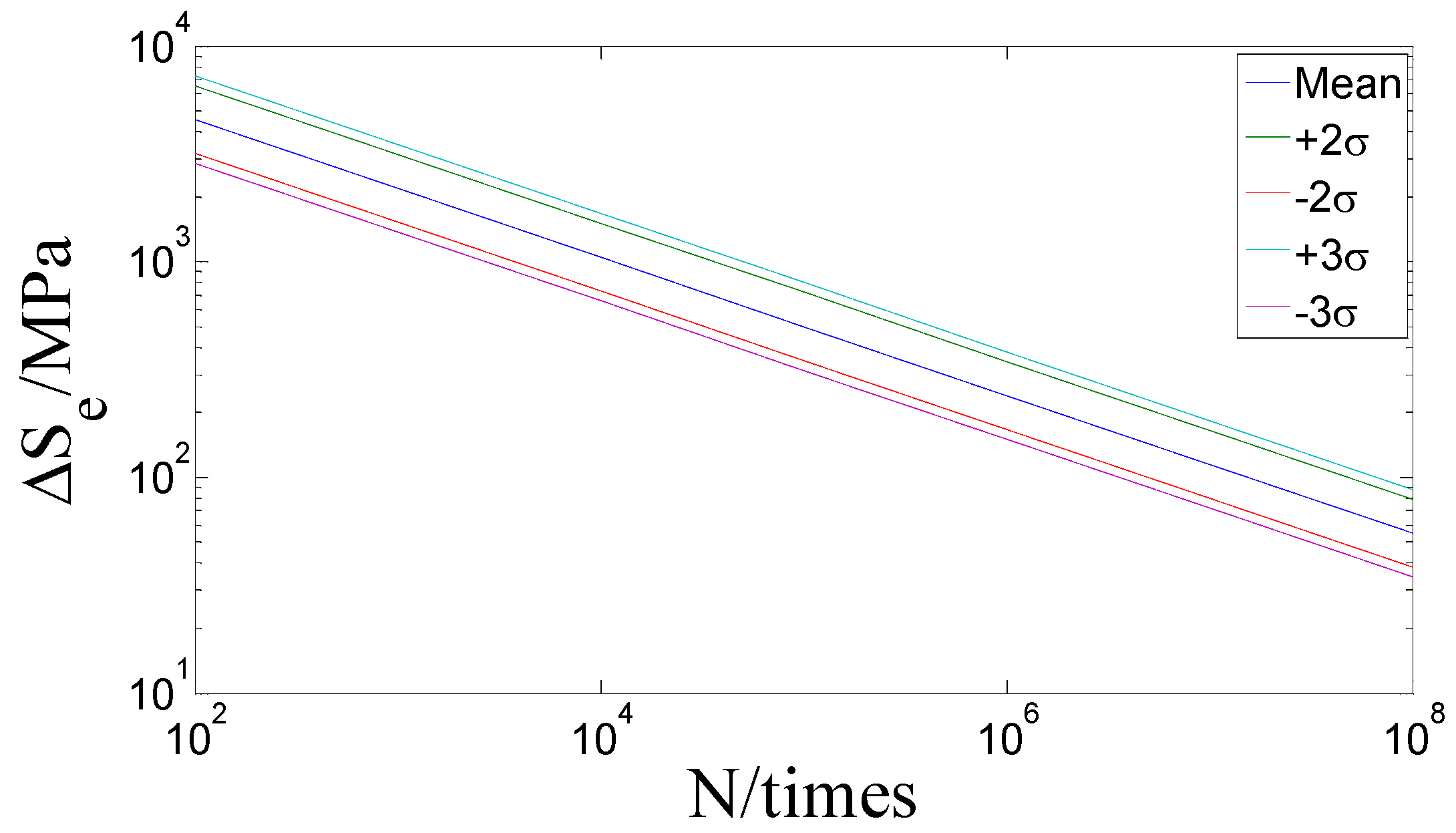
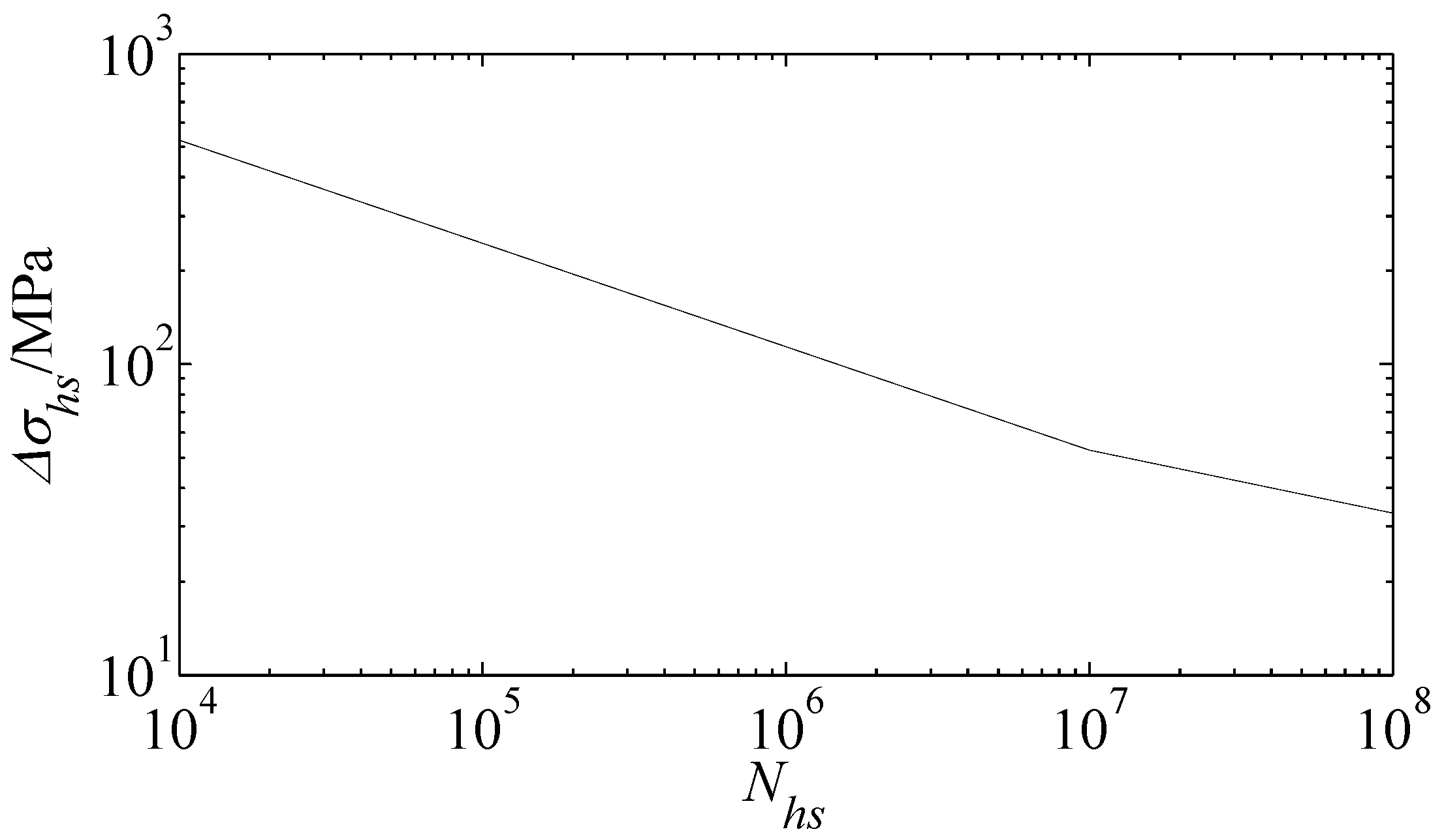
After defining the equivalent structural stress , the master S-N curve is defined in the form of:

$$\Delta S_e=C·N^h$$

(16)

where C and h are constants, as shown in

Table 1. Parameters for master S-N curve.

Statistical Basis	C	h
Mean	19930.2	0.32
+2σ	28626.5
−2σ	13875.8
+3σ	31796.1
−3σ	12492.6

. σ represents the standard derivation defined with respect to cycle to failure in log scale. Different curves based on the corresponding statistical basis are illustrated in Figure 8. Here, the mean curve is selected, so C is 19930.2 and h is 0.32.

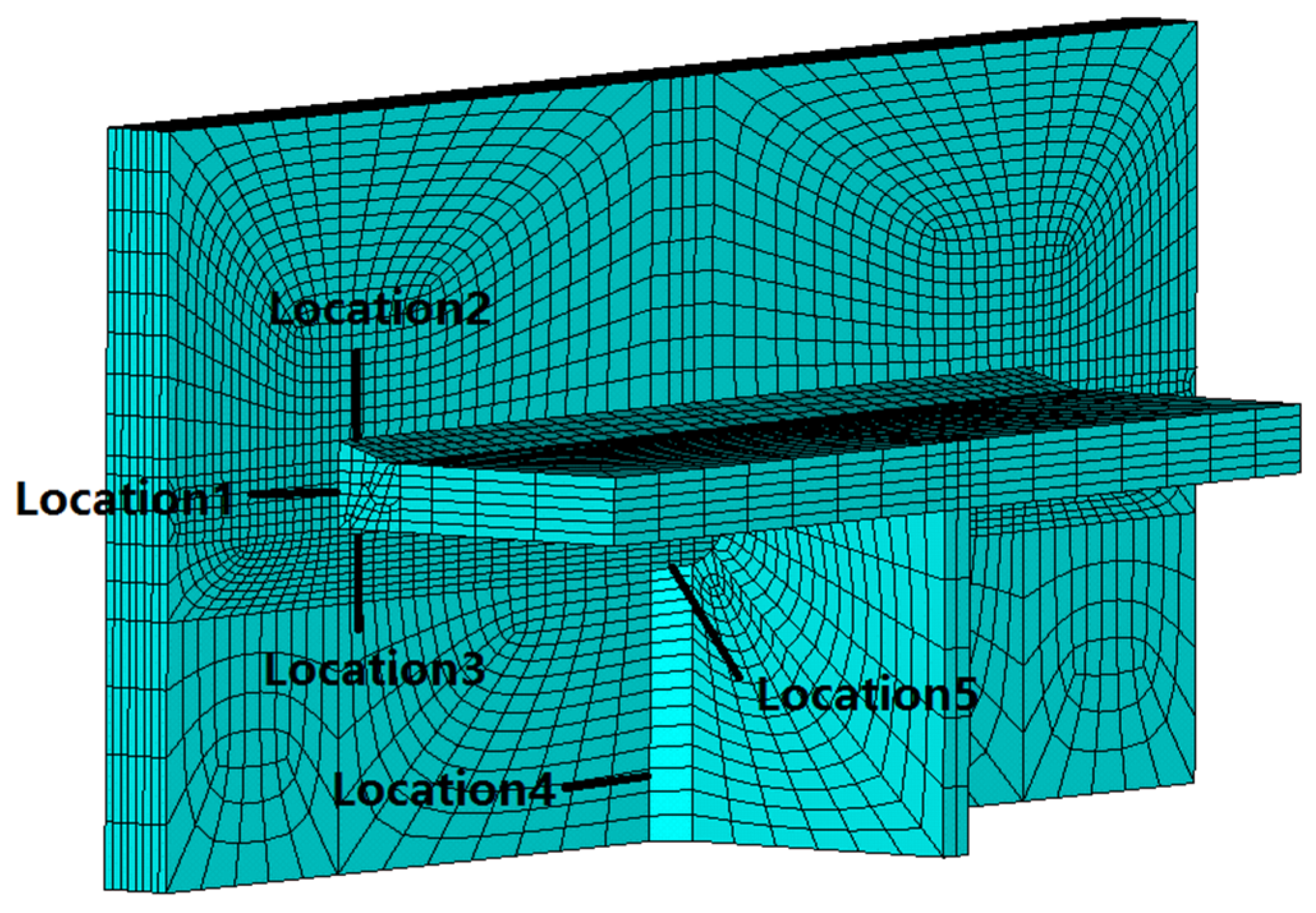
In the local weld model which consists of a butt weld near the flange plate and a fillet weld near the web plate, five typical locations near the welds are selected, which are the lateral weld toe of the butt weld on the column (Location 1), upper weld toe of the butt weld on the column (Location 2), lower weld toe of the butt weld on the column (Location 3), the lateral weld toe of the fillet weld (Location 4) and the upper side of the fillet weld (Location 5), as shown in Figure 9. These locations are usually regarded as the dangerous locations where stress concentration exists.

Based on the modified equivalent structural stress formulae and the master S-N curve stated above, the fatigue assessment of these five locations is carried out as follows.

First, by area map and area operation technology involved in ANSYS, the integral parts in Equations (10) and (11) can be obtained and thus the membrane stress ${\mathsf{\sigma }}_{m3D}$ and bending stress ${\mathsf{\sigma }}_{b3D}$ can be calculated, which are variables related to time. According to Equation (12), the structural stress ${\mathsf{\sigma }}_{s3D}$ time-history can be obtained. Finally, the time-history of structural stress ${\mathsf{\sigma }}_{s3D}$ is converted to the time-history of the equivalent structural stress $\Delta S_e$ according to Equation (13).

Second, according to rain-flow counting method and Palmgren–Miner linear accumulating damage rule, the effective equivalent structural stress range $\Delta S_{eq}$ which produces the same amount of fatigue damage during this 50 s time as the time-history of the equivalent structural stress $\Delta S_e$ does is obtained according to Equation (19). The cycle number n₅₀ during this 50 s time can also be obtaiend according to rain-flow counting method. As the formula of $\Delta S_{eq}$ based on equivalent structural stress method is a little different from that based on hot spot stress method, the deduction procedure is detailed as follows.

When undergoing varied amplitude loading, the accumulating damage is:

$$D_1={\displaystyle \sum }_{i=1}^k\frac{n_i}{N_i}={\displaystyle \sum }_{i=1}^k\frac{n_i}{\sqrt[h]{\frac{\Delta S_{ei}}{C}}}$$

(17)

where $\Delta S_{ei}$ is the i-th equivalent structural stress range causing fatigue damage in the stress spectrum, $n_i$ is the number of cycles under stress range $\Delta S_{ei}$, and N_i is the number of failure cycles under the action of $\Delta S_{ei}$.

When undergoing constant amplitude loading, the accumulating damage is:

$$D_2=\frac{{{\displaystyle \sum }}_{i=1}^k{n}_i}{N}=\frac{{{\displaystyle \sum }}_{i=1}^k{n}_i}{\sqrt[h]{\frac{\Delta S_{eq}}{C}}}$$

(18)

To make these two equivalent, which means $D_1=D_2$, the effective stress range based on equivalent structural stress method is calculated as:

$$\Delta S_{eq}=C·{\left(\frac{{{\displaystyle \sum }}_{i=1}^k{n}_i}{{{\displaystyle \sum }}_{i=1}^k\frac{n_i}{\sqrt[h]{\raisebox{1ex}{$\Delta S_{ei}$}\!\left/ \!\raisebox{-1ex}{$C$}\right.}}}\right)}^h$$

(19)

Combined with the master S-N curve stated above, the number of failure cycles $N_{eq}$ under the action of $\Delta S_{eq}$ can be calculated by Equation (20) and the fatigue damage during this 50 s $D_{50}$ is obtained by Equation (21):

$$N_{eq}=\sqrt[h]{\frac{\Delta S_{eq}}{C}}$$

(20)

$$D_{50}=\frac{n_{50}}{N_{eq}}$$

(21)

By extending it to the time of one year, the annual fatigue damage $D_{annual}$ and fatigue life $T$ of these six locations can be assessed by Equations (22) and (23):

$$D_{annual}=\raisebox{1ex}{$31536000$}\!\left/ \!\raisebox{-1ex}{$50$}\right.·D_{50}$$

(22)

$$T=\frac{1}{D_{annual}}$$

(23)

7. Results

The fatigue life assessment results obtained as the procedures detailed above are shown in

Table 2. Fatigue assessment result based on equivalent structural stress method.

Location	$\mathbf{\Delta }{\mathit{S}}_{\mathit{e}\mathit{q}}/\mathbf{M}\mathbf{P}\mathbf{a}$	${\mathit{D}}_{50}$	${\mathit{D}}_{\mathit{a}\mathit{n}\mathit{n}\mathit{u}\mathit{a}\mathit{l}}$	$\mathit{T}$/year
1	9.200	$5.986\times {10}^{-9}$	0.0038	265
2	6.103	$1.682\times {10}^{-9}$	0.0011	943
3	6.478	$2.001\times {10}^{-9}$	0.0013	792
4	0.058	7.887$\times {10}^{-16}$	4.974$\times {10}^{-10}$	2.010 $\times {10}^9$
5	1.463	1.964 $\times {10}^{-11}$	1.239 $\times {10}^{-5}$	8.074 $\times {10}^4$

.

In Table 2, it can be seen that the fatigue damage of the fillet weld connecting the web plate and the column is much smaller than that of the butt weld connecting the upper beam flange plate and column, which means in high-rise steel braced frame structure the butt weld connecting the upper beam flange plate and column is more dangerous in regards to fatigue damage. By comparing fatigue life and damage of Locations 1–3, it can be discovered that the fatigue life of Location 1 is the shortest, which means the lateral weld toe of the butt weld connecting the upper beam flange plate and column is the most dangerous location, whose fatigue life is 265 years, which meets the engineering design demands.

8. Discussion

After the results have been obtained, further discussion and verification is necessary. In this section, the effect of meshing style on the calculating results is discussed to verify the mesh-insensitive quality. Furthermore, fatigue assessments based on hot spot stress and nominal stress are performed and comparisons are made to verify the results.

8.1. Element Type and Size Impact Analysis

Since fatigue life assessment based on equivalent structural stress method is insensitive to meshing style, it is indispensable to verify the negligible effect of changing element type and size on the computing results near the weld. If the verification is failed, it means the results are incorrect.

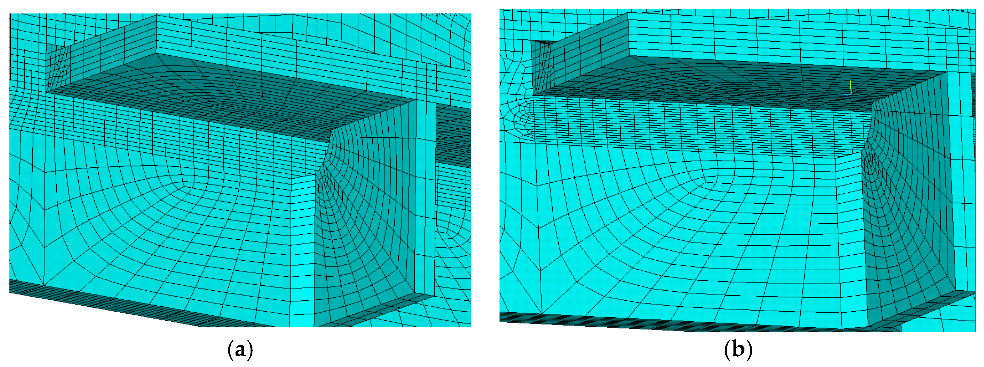
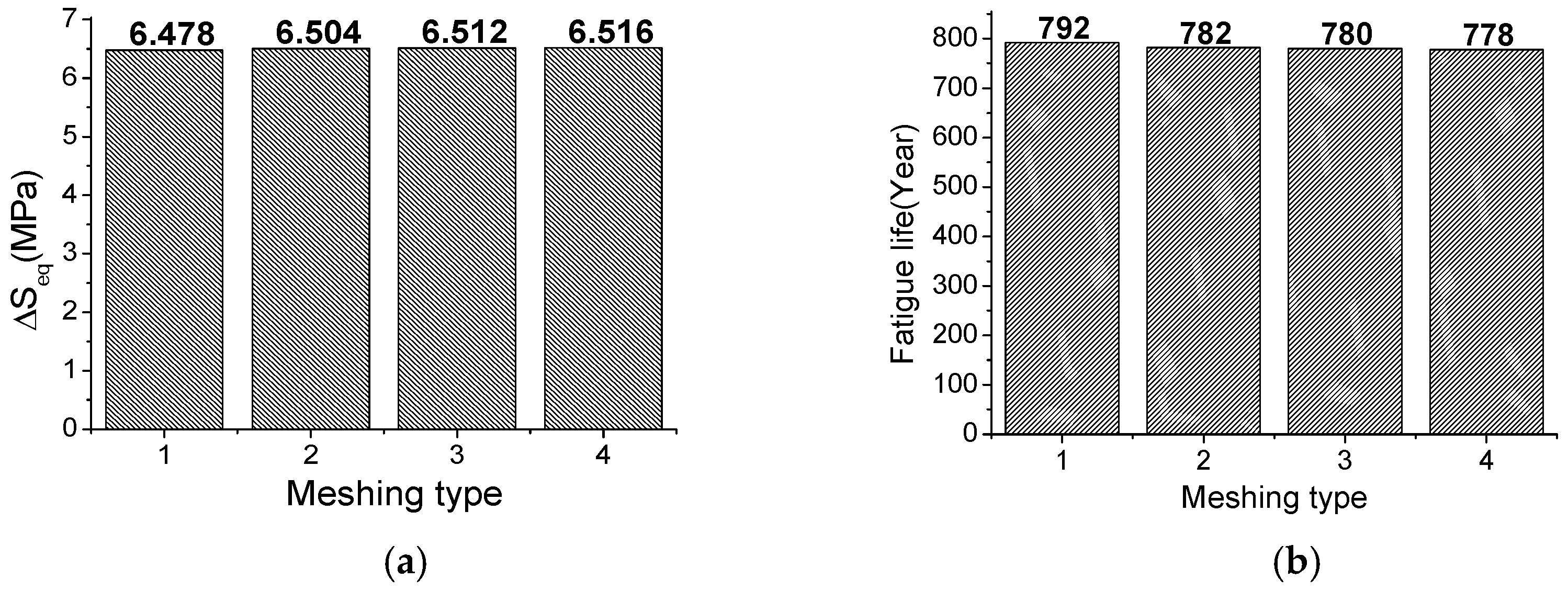
Take Location 3 as an example, for the alteration of meshing styles is relatively easy and convenient. Different element types, which contain linear element SOLID45 (8 nodes) and quadratic element SOLID95 (20 nodes), or different meshing sizes, which contain 1 mm and 2 mm in the vicinity of Location 3 (in the direction perpendicular to the weld seam) as shown in Figure 10 are adopted, respectively.

Table 3. Different meshing types.

Meshing Type	Element Type	Number of Nodes	Size Dimension/mm
1	SOLID45	8	2
2	SOLID45	8	1
3	SOLID95	20	2
4	SOLID95	20	1

lists the description of these four meshing types. Time history analysis is performed as previously stated. The results of effective equivalent structural stress range $\Delta S_{eq}$ and fatigue life are illustrated in Figure 11.

According to the results obtained above, it can be found that with the decreasing element size dimension and the use of high order elements, the effective equivalent structural stress range and fatigue life assessment results based on equivalent structural stress method keep almost invariant, which verifies that the equivalent structural stress method is indeed mesh-insensitive.

8.2. Results Compared with Hot Spot Stress Method

As hot spot stress theory has been widely used in fatigue assessment in the field of civil engineering and proven to be quite reliable. It is necessary to compare the results obtained by hot spot stress method and equivalent structural stress method so that the results obtained by equivalent structural stress can be verified.

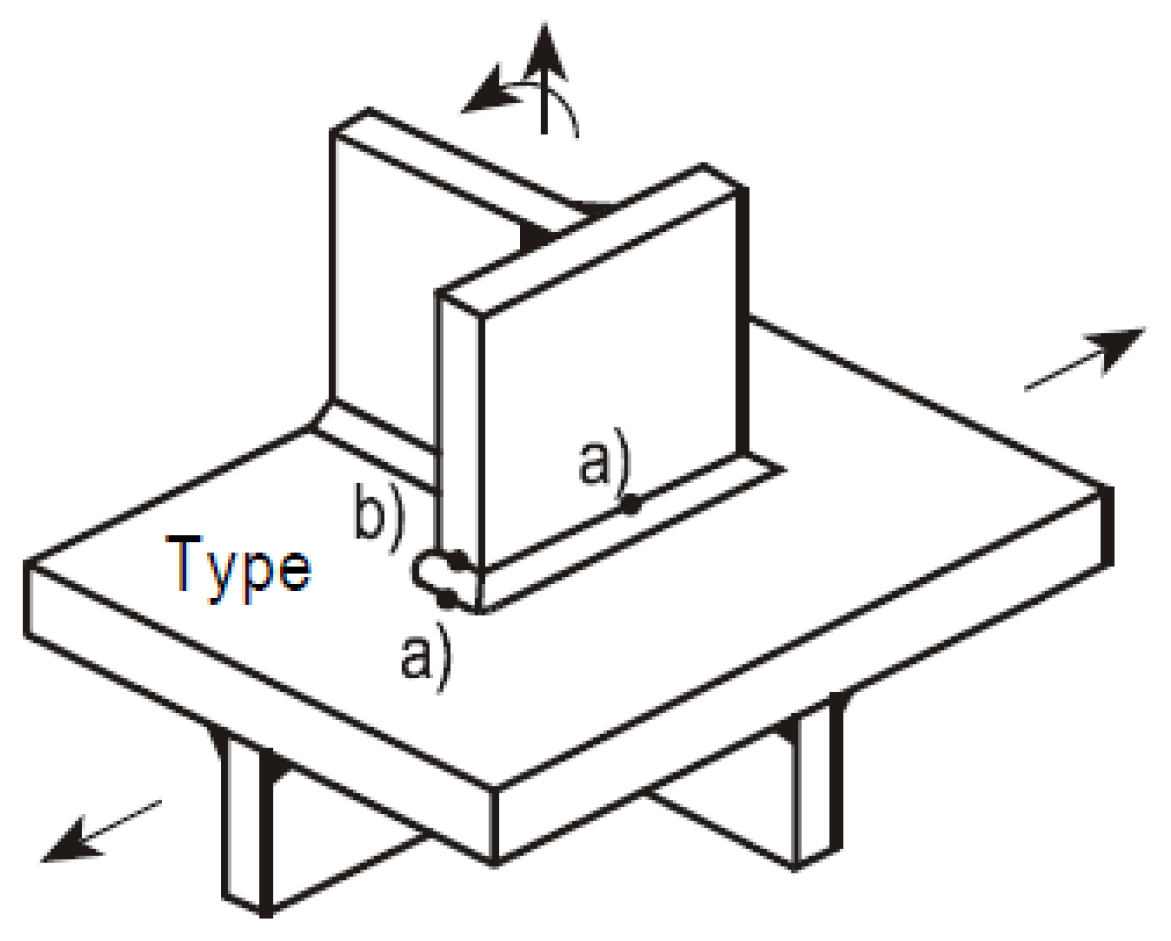
The hot spot stress represents the structural stress at the hot spot, which includes all stress raising effects of a structural detail and excludes all stress concentrations due to the local weld profile itself. There are mainly two types of hot spot and they can be defined as Type a, which is hot spot stress transverse to weld toe on plate surface, and Type b, which is hot spot stress transverse to weld toe at plate edge, as illustrated in Figure 12.

When hot spot stress is used to calculate the structural stress, a surface stress extrapolation can be defined. For Type a hot spot, a linear extrapolation is adopted, where the hot spot stress ${\mathsf{\sigma }}_{\mathrm{hsa}}$ can be calculated according to the stress of two reference points which are located 0.4t and 1.0t away from the hot spot (${\mathsf{\sigma }}_{x_1},{\mathsf{\sigma }}_{x_2}$), where t is the thickness of the adjacent plate, as defined in Equation (24):

$${\mathsf{\sigma }}_{\mathrm{hsa}}=1.67{\mathsf{\sigma }}_{x_1}-0.67{\mathsf{\sigma }}_{x_2}$$

(24)

For Type b hot spot, a linear extrapolation of three reference points is adopted, where the hot spot stress ${\mathsf{\sigma }}_{\mathrm{hsb}}$ can be calculated according to the stress of three reference points which are located 4 mm, 8 mm and 12 mm away from the hot spot (${\mathsf{\sigma }}_{x_1}^{\prime },{\mathsf{\sigma }}_{x_2}^{\prime },{{\mathsf{\sigma }}_{x_3}}^{\prime }$), as defined in Equation (25):

$${\mathsf{\sigma }}_{\mathrm{hsb}}=3{{\mathsf{\sigma }}_{x_1}}^{\prime }-3{{\mathsf{\sigma }}_{x_2}}^{\prime }+{{\mathsf{\sigma }}_{x_3}}^{\prime }$$

(25)

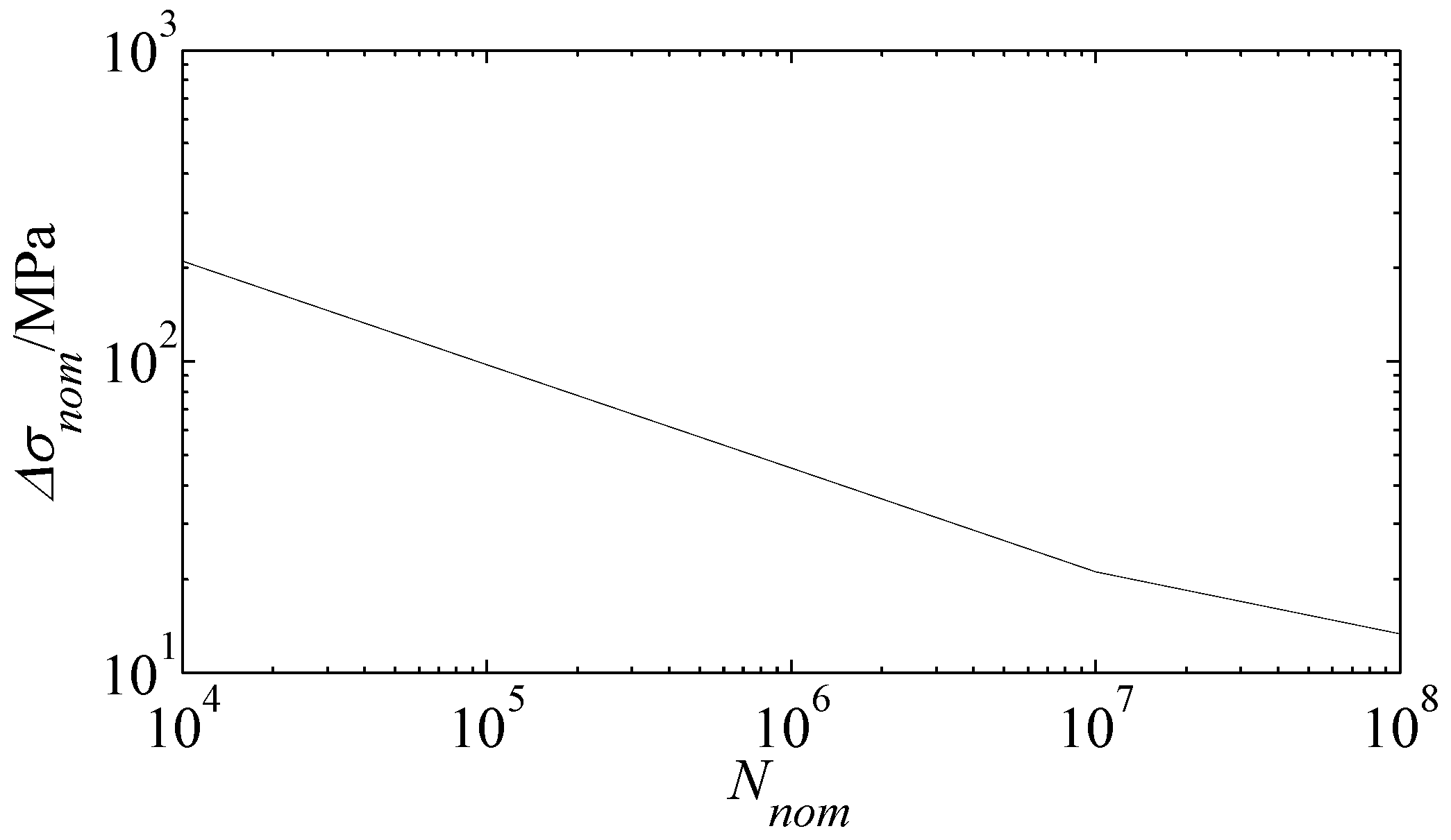
According to the IIW Recommendations [15], FAT90 curve is found to be the most proper S-N curve, which is shown as Equation (26) and illustrated in Figure 13.

$$\Delta {{\mathsf{\sigma }}_{hs}}^{m^{\prime }}{N}_{hs}=C_{hs}$$

(26)

where $\Delta {\mathsf{\sigma }}_{hs}$ is the hot spot stress range, $N_{hs}$ is the number of failure cycles under the action of stress range $\Delta {\mathsf{\sigma }}_{hs}$, $C_{hs}$ is a constant and m’ is the negative reciprocal of S-N curve slope in double logarithmic coordinates, which can be found in

Table 4. Parameters for FAT90 curve.

FAT	Knee Point Stress Range $\mathbf{\Delta }{\mathsf{\sigma }}_{\mathit{k}\mathit{p}}$	${\mathit{N}}_{\mathit{h}\mathit{s}}\le {10}^7$		${\mathit{N}}_{\mathit{h}\mathit{s}}>{10}^7$
		${\mathit{m}}^{\prime }$	${\mathit{C}}_{\mathit{h}\mathit{s}}$	${\mathit{m}}^{\prime }$	${\mathit{C}}_{\mathit{h}\mathit{s}}$
90	52.7 MPa	3	$1.458\times {10}^{12}$	5	$4.065\times {10}^{15}$

.

After the time-history analysis is conducted and the hot spot stress is obtained as the procedure above, the rain-flow counting method and Palmgren–Miner linear accumulating damage rule are utilized once again to convert the varied amplitude range to an effective range, which is shown as Equation (27). The cycle number $n_{50hs}$ during this 50 s can also be obtained.

$$\Delta {\mathsf{\sigma }}_e={\left[\frac{{{\displaystyle \sum }}_{i=1}^k{n_i}^{\prime }{\left(\Delta {\mathsf{\sigma }}_{hsi}\right)}^{m^{\prime }}}{N_{eqhs}}\right]}^{\raisebox{1ex}{$1$}\!\left/ \!\raisebox{-1ex}{$m^{\prime }$}\right.}$$

(27)

where $N_{eqhs}$ is the cycle number during this 50 s, $\Delta {\mathsf{\sigma }}_{hsi}$ is the i-th hot spot stress range causing fatigue damage in the stress spectrum, and ${n_i}^{\prime }$ is the number of cycles under stress range $\Delta {\mathsf{\sigma }}_{hsi}$.

Based on the effective hot spot stress range $\Delta {\mathsf{\sigma }}_e$, the number of failure cycles $N_{hs}$ under the action of $\Delta {\mathsf{\sigma }}_{hs}$ can be calculated by Equation (26) and the fatigue damage during this 50 s can be obtained by Equation (21). Thus, the annual fatigue damage and fatigue life can be calculated according to Equations (22) and (23) and the results are shown in

Table 5. Fatigue assessment result based on hot spot stress method.

Location	Type of Hot Spot	$\mathbf{\Delta }{\mathsf{\sigma }}_{\mathit{e}}/\mathbf{M}\mathbf{P}\mathbf{a}$	${\mathit{D}}_{50\mathit{h}\mathit{s}}$	${\mathit{D}}_{\mathit{a}\mathit{n}\mathit{n}\mathit{u}\mathit{a}\mathit{l}\mathit{h}\mathit{s}}$	${\mathit{T}}_{\mathit{h}\mathit{s}}$/Year
1	a	12.155	$1.005\times {10}^{-8}$	0.0032	315
2	a	9.367	$2.733\times {10}^{-9}$	0.0009	1160
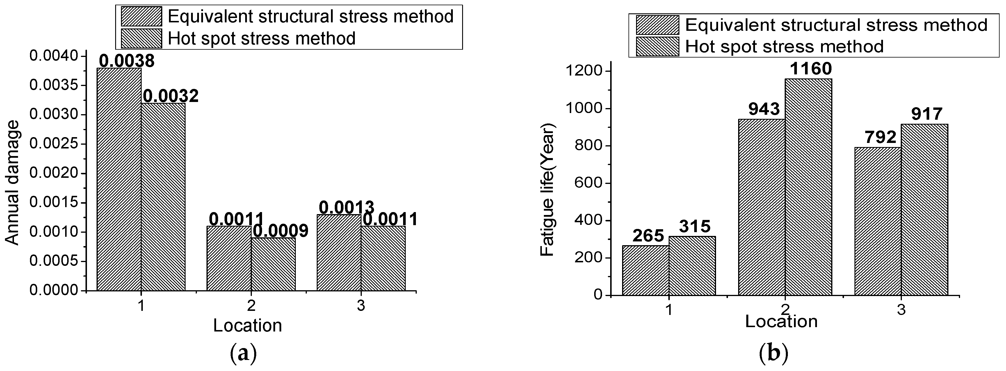
3	a	9.819	$3.457\times {10}^{-9}$	0.0011	917

. As can be concluded from the results obtained by equivalent structural stress method above, the fatigue life of the fillet weld connecting the web plate and the column is much longer than that of the butt weld connecting the upper beam flange plate and column, so, for simplicity, only the three locations near the butt weld connecting the upper beam flange plate and column are calculated in hot spot stress method. Figure 14 illustrates the results based on equivalent structural stress and hot spot stress.

According to Table 5 and Figure 14, it can be found that the discrepancy of results obtained by hot spot stress and equivalent structural stress are mostly around 15%, which meets engineering demands. The discrepancy maybe mainly stems from the complicated stress state involved in large-scale structures, which are usually multi-axial stress state, while in small-scale welded joint test specimens the stress state is relatively simple, which is usually single-axial stress state, so the fatigue assessment using different methods agrees perfectly with each other. It can be found that the fatigue damage calculated by equivalent structural stress is higher than that calculated by hot spot stress, which means the fatigue assessment by equivalent structural stress method is more conservative and tends to be safer when engineering structures are designed. Actually, compared with hot spot stress method, the two greatest advantages of equivalent structural stress method lie in the mesh-insensitive quality, which is very important when large-scale engineering structures are dealt with, and the capability of unifying different curves into one master S-N curve, which can avoid the confusion when the desired curve needs to be selected.

8.3. Results Compared with Nominal Stress Method

As most fatigue assessment in the field of civil engineering is based on nominal stress, it is necessary to compare the results obtained by nominal stress and equivalent structural stress so that the advantage and disadvantage can be concluded.

In nominal stress assessment, the multi-scale FE model is replaced by a global one, as shown in Figure 15, where beams and columns are completely simulated by element BEAM188 and the local model with element SOLID45 is no longer necessary. It is no doubt that analysis using this global model costs far less computing resources and time, at a cost of the confusion of selecting the proper S-N curve and inability of considering the local concentration. According to the IIW Recommendations [15], as there are so many curves involved during the selection of a desirable S-N curve, it seems that only approximate welded joint detail can be found. Finally, FAT36 curve is found to be the most proper S-N curve, which is described in

Table 6. Description of FAT36 curve.

FAT36 Curve	Description
	Splice of rolled section with intermediate plate, fillet welds, weld root crack. Analysis base on stress in weld throat.

and shown as Equation (28) and illustrated in Figure 16.

$$\Delta {{\mathsf{\sigma }}_{nom}}^{m^{\prime }}{N}_{nom}=C_{nom}$$

(28)

where $\Delta {\mathsf{\sigma }}_{nom}$ is the nominal stress range, $N_{nom}$ is the number of failure cycles under the action of stress range $\Delta {\mathsf{\sigma }}_{nom}$, $C_{nom}$ is a constant and m’ is the negative reciprocal of S-N curve slope in double logarithmic coordinates, which can be found in

Table 7. Parameters for FAT36 curve.

FAT	Knee Point Stress Range $\mathbf{\Delta }{\mathsf{\sigma }}_{\mathit{k}\mathit{p}}$	${\mathit{N}}_{\mathit{n}\mathit{o}\mathit{m}}\le {10}^7$		${\mathit{N}}_{\mathit{n}\mathit{o}\mathit{m}}>{10}^7$
		${\mathit{m}}^{\prime }$	${\mathit{C}}_{\mathit{n}\mathit{o}\mathit{m}}$	${\mathit{m}}^{\prime }$	${\mathit{C}}_{\mathit{n}\mathit{o}\mathit{m}}$
36	58.5 MPa	3	$2\times {10}^{12}$	5	$6.851\times {10}^{15}$

.

Based on FAT36 curve, the nominal stress can be determined by elementary theories of structural mechanics based on linear-elastic behavior. Nominal stress ${\mathsf{\sigma }}_{nom}$ is the average stress in the plate at weld toe of the structural detail, which can be defined as:

$${\mathsf{\sigma }}_{nom}=\frac{N}{A}+\frac{M_x}{I_x}+\frac{M_y}{I_y}$$

(29)

where N is the axial force, A is the section area of the plate, M_x and M_y are the moment in the two mutually perpendicular directions on the plate section, and I_x and I_y are the inertia moment of the plate section. These parameters, which are all time series, can be obtained through the global FE model. With the same wind time series utilized, time history analysis is performed.

The rain-flow counting method and Palmgren–Miner linear accumulating damage rule are utilized once again to convert the varied amplitude range to an effective range, which is shown as Equation (30), and cycle number $n_{50nom}$ during this 50 s can be obtained:

$$\Delta {\mathsf{\sigma }}_{nom}={\left[\frac{{{\displaystyle \sum }}_{i=1}^k{n_i}^{\prime }{\left(\Delta {\mathsf{\sigma }}_{nomi}\right)}^{m^{\prime }}}{N_{eqnom}}\right]}^{\raisebox{1ex}{$1$}\!\left/ \!\raisebox{-1ex}{$m^{\prime }$}\right.}$$

(30)

where $N_{eqnom}$ is the cycle number during this 50 s, $\Delta {\mathsf{\sigma }}_{nomi}$ is the i-th nominal stress range causing fatigue damage in the stress spectrum, and ${n_i}^{\prime }$ is the number of cycles under stress range $\Delta {\mathsf{\sigma }}_{nomi}$.

Based on the effective nominal stress range $\Delta {\mathsf{\sigma }}_{nom}$, the number of failure cycles $N_{nom}$ under the action of $\Delta {\mathsf{\sigma }}_{nom}$ can be calculated by Equation (28) and the fatigue damage during this 50 s can be obtained by Equation (21). Thus, the annual fatigue damage $D_{annualnom}$ and fatigue life $T_{nom}$ can be calculated according to Equations (22) and (23) and the results are shown in

Table 8. Fatigue assessment using different methods.

Method	Location	${\mathit{D}}_{50\mathit{n}\mathit{o}\mathit{m}}$	${\mathit{D}}_{\mathit{a}\mathit{n}\mathit{n}\mathit{u}\mathit{a}\mathit{l}\mathit{n}\mathit{o}\mathit{m}}$	${\mathit{T}}_{\mathit{n}\mathit{o}\mathit{m}}$/Year
Nominal stress	Global	$1.377\times {10}^{-10}$	4.342 $\times {10}^{-5}$	2.3 $\times {10}^4$
Equivalent structural stress	Location 1	$5.986\times {10}^{-9}$	0.0038	265
	Location 4	7.887 $\times {10}^{-16}$	4.974 $\times {10}^{-10}$	2.010 $\times {10}^9$

.

According to Table 8, it can be found that the result obtained by nominal stress varies greatly from and falls in between the results based on equivalent structural stress method of different locations of the weld. It means nominal stress method considers the weld in a more global way, which averages all the stress on the weld plate section and it cannot consider the local stress concentration accurately while in equivalent structural stress method, the fatigue life of different parts vary greatly and in the stress concentration zone, the fatigue life assessed is far less than that in other parts. As a result, relative large discrepancy exists between the fatigue life result of the stress concentration zone based on equivalent structural stress method and that averaged in the whole section by nominal stress method. This phenomenon, which has been found in the relevant literature [16], is extremely obvious in large-scale structures, although in small-scale welded joint tests, the two results can mostly agree well with each other. This may be because of the complicated stress state involved in large-scale structures while in small-scale welded joint tests the stress state is relatively simple.

Generally speaking, compared with the fatigue assessment based on equivalent structural stress, the fatigue assessment based on nominal stress tends to be dangerous due to its less consideration of local stress concentration. However, nominal stress method is still widely used in practical for its great convenience of FE modeling and fast computing speed to estimate the fatigue life, which is especially important involving complicated engineering project.

9. Conclusions

This paper has presented the fatigue life assessment of a typical steel high-rise steel braced frame structure using the equivalent structural stress method. By establishing multi-scale FE model and time-history analysis, fatigue assessment is performed using equivalent structural stress method. As a result, Location 1, which is lateral weld toe of the butt weld connecting the upper beam flange plate and column, is found to be the most dangerous location and is likely subjected to fatigue damage. This can provide reference to the design of steel high-rise steel braced frame structures. Furthermore, the comparison of the results obtained by equivalent structural stress and hot spot stress show fatigue damage calculated by equivalent structural stress is higher, which means the fatigue assessment by equivalent structural stress method is more conservative and tends to be safer. Meanwhile, the results based on nominal stress reflects that nominal stress method considers the weld in a more global way, which averages all the stress on the weld plate section and cannot take into account the local stress concentration near the welds accurately. However, in nominal stress assessment, only global FE model is required and the computing time is much shorter than that in equivalent structural stress or hot spot stress. Therefore, nominal stress method, hot spot stress method and equivalent structural stress method have their own advantages and disadvantages and selection needs to be determined according to detailed circumstances. Generally speaking, in fatigue assessment of large-scale complex structures, nominal stress method is recommended to be used to study the fatigue damage trend, and is especially suitable for looking for the critical components regarding fatigue failure in large-scale structures. Equivalent structural stress method or hot spot stress method if the conditions are allowed (computing resources and time are abundant) is recommended to be used to analyze the fatigue life accurately. Furthermore, the methodology stated in this paper can be applied similarly to any high-rise steel structure, including mast structures and tower structures with welded joints, thus providing reference to wind-induced fatigue assessment of any high-rise steel structure.