Analysis of MPPT Failure and Development of an Augmented Nonlinear Controller for MPPT of Photovoltaic Systems under Partial Shading Conditions

Abstract

The output–voltage–power curves of photovoltaic (PV) arrays exhibit complex multi-peak shapes when local shading occurs. The existing maximum power point tracking (MPPT) algorithms to solve this multi-peak problem do not consider the possibility of tracking failures due to the time of the irradiance change. In this study, first, the reason for the failure of the global MPPT (GMPPT) algorithm is analyzed based on the PV array mathematical model and its output characteristics under partial shading conditions; then, in order to estimate the MPP voltage, an artificial neural network (ANN) is trained using environmental information such as irradiance. A hybrid MPPT method using an augmented state feedback precise linearization (AFL) controller combined with an ANN is proposed to solve problems such as the shift of the static operating point of the DC/DC boost converter. Finally, numerical simulations are conducted to validate the proposed method and eliminate the possibility of MPPT failure. The proposed hybrid MPPT method is compared with the conventional perturb and observe (P & O) method and the improved P & O method through simulations. Using the proposed neural network and nonlinear control strategy, the MPP can be tracked rapidly, accurately, and statically, proving that the method is feasible and effective.

1. Introduction

Global energy consumption has increased noticeably due to the increase in the population. The sustainable use of renewable energy solves one of the major concerns of the world community, since the amount of fossil energy sources is no longer sufficient [1]. Energy generated from photovoltaic (PV) systems is inexhaustible; hence, PV systems are suitable candidates for a long-term, reliable, and environmentally friendly source of electricity [2]. The output power of a PV systems varies with the intensity of the solar irradiance and the environmental temperature. Due to the nonlinear current–voltage (I–V) characteristics of the solar cell, there is a unique maximum power point (MPP) on the power–voltage (P–V) curve. Global maximum power point tracking (GMPPT) is one of the basic measures to improve the overall efficiency of the PV power generation systems. However, real environments experience partial shading, which is a condition whereby a portion of the PV module (or array) is shaded, while the other parts remain uniformly irradiated. When a PV array is subjected to partial shading, a considerable amount of energy is lost because the shaded module is short-circuited by its bypass diode. This forces its voltage, and consequently power, to be reduced to zero and the P–V curve exhibits a complex multi-peak shape. In this case, the traditional algorithms using gradient information, such as the perturb-and-observe (P & O) and incremental conductance (INC) algorithms, become invalid [3,4,5,6,7,8].

In the last decade, several researchers have compared various MPPT techniques [9,10], focusing on the P–V characteristics [11,12,13,14,15], models [16,17,18,19], and methods [20,21,22,23,24,25,26,27,28,29,30,31,32,33] to track the maximum power of PV modules/arrays under partial shading conditions (PSC). The research on the PV output characteristics is mainly focused on the analysis of failure, power loss, and voltage variations in the MPPT method under the PSC. The research on the PV model mainly concentrates on a unified model of the PV array and an accurate model of the PV unit under complex environments. In general, the results of the studies on PV output characteristics and models are often fed back for updating the GMPPT algorithm; thus, they are significant for the applications of the PV system.

The maximum power tracking algorithms, which are the core of the PV power generation systems, can be broadly divided into three categories:

In the first category, the GMPP can be obtained by traversing all the maximum points in the PV array, which are the local maximum power points (LMPPs), and then sorting this maximum group [20,21,22]. The advantage is that the GMPP can be found accurately, and the algorithm is simple and stable; however, the optimization process is slow, redundant, and wastes hardware and software resources.

In the second category, the region of maximum power is determined according to the PV and model characteristics, and the multi-peak problem is transformed into a unimodal problem of the region. Then, the traditional method is used to track the MPP [23,24,25,26]. The advantage of the methods in this category is that they can reduce the traversal region; however, they have a higher dependency on the analysis of the local shadow models and output characteristics, which means that the determination of the MPP region is difficult and the robustness is poor.

In the third category, using a heuristic and intelligent optimization algorithm, the global maximum power of the PV system is directly calculated using an iterative method [27,28,29,30,31,32,33], to achieve MPPT. The advantages of these methods are that they do not depend on the model or PV characteristics, and can even update the algorithm through online follow-ups and self-learning. However, it is difficult to deal with the problems of GMPPT under frequent, continuous, and rapid changes in irradiance, because the iterative process is usually slow and can be easily trapped in a local optimal solution. In addition, the accuracy of the steady-state solution is not high.

In summary, a large number of scholars have conducted in-depth studies on the local shadowing in PV GMPPT. However, most of the algorithms still have problems such as slow global search speed, local optimality, and over-dependence on system models. In addition, the verification methods for these algorithms are based on the static multi-peak problem, and they ignore the possible MPPT failures caused by irradiance changes. To the best of the authors’ knowledge, there has been no published paper presenting a framework using an intelligent hybrid method for PV systems in the grid-connected mode. The major contributions of this paper, toward overcoming the drawbacks of the above references, are outlined below:

(1)

The output characteristics of the PV arrays are analyzed using the PV array model under PSC, and the V–P curve is found to demonstrate a multi-peak trend. The reasons for the failure of the conventional MPPT algorithm are analyzed under the premise of rapid and continuous irradiance changes.

(2)

For the MPPT failures caused by the timings of the irradiance changes, this paper proposes a hybrid MPPT method that uses an artificial neural network (ANN) to estimate the MPP and an augmented state feedback precise linearization (AFL) controller for the DC/DC converter to meet the fast and frequent changes in irradiance.

(3)

Considering the influence of the multi-peak output of the PV array on the small signal of the DC/DC converter under PSC, this paper designs a nonlinear control method with precise state feedback linearization.

The remainder of this paper is organized as follows: Section 2 presents the structure of the PV system proposed in this paper, a nonlinear mathematical model of the PV array under PSC, and the reason for the failure of GMPPT under PSC. Section 3 introduces the proposed training results of the ANN structure used for MPPT, based on the environment information, and analyzes the error in the network. Section 4 presents an AFL nonlinear controller to track the output reference voltage of the ANN over a wide range, based on the nonlinear mathematical analysis of the DC/DC converter, and designs the controller of the DC/AC converter to accomplish the whole scheme of PV system connection to grid. Section 5 illustrates the performance of the proposed solution using detailed simulations executed under various conditions to validate the effectiveness of the hybrid MPPT method proposed in this paper. Simulations for the comparison of the proposed MPPT method with the conventional P & O method and the improved P & O method are also illustrated. The conclusions are presented in Section 6, which is the last part of this paper.

2. Grid-Connected PV Generation System

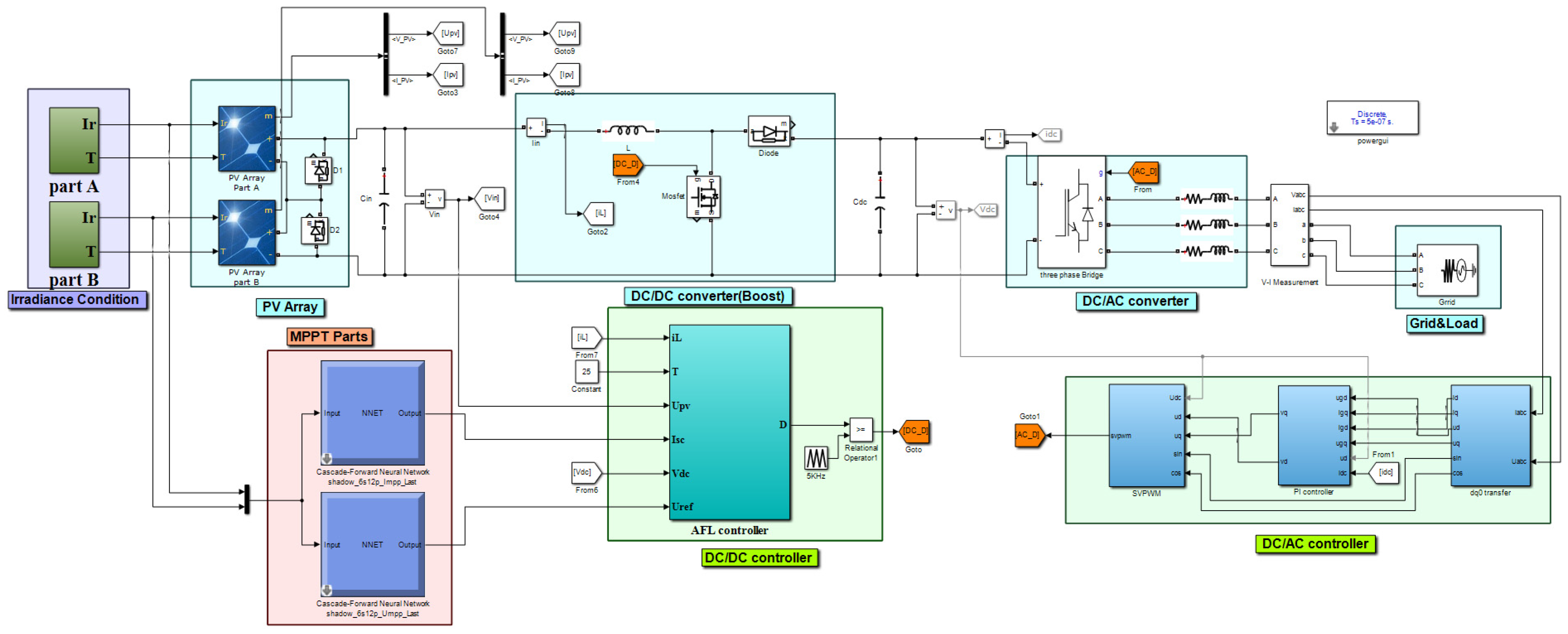
2.1. Structure of the Proposed System

Irradiance, temperature, and other environmental information present nonlinear characteristics with respect to the PV output power. The output-voltage–power curves of the PV arrays exhibit complex multi-peak shapes when local shading occurs. Because the ANN has the capability to be used in nonlinear applications and can respond rapidly to changes in reference, its usage in different areas has been growing. An ANN does not require reprogramming as it is based on a learning process. Therefore, in this paper, the irradiances of different solar cells are detected to train the ANN controller to obtain an MPP reference.

The power electronic converter model is a typical nonlinear system model. Conventional controllers such as the PI controllers based on small-signal modeling cannot track the reference rapidly and precisely when the converter quiescent operating point shifts over a wide dynamic range. The static operating point of the boost DC/DC converter will vary widely under PSC. This paper proposes an AFL controller based on the DC/DC converter to solve the problems that exist in conventional controllers.

Figure 1 shows the structure of a grid-connected PV system in which a PV generator interacts with a DC/DC converter controlled by an MPPT algorithm using ANN. By detecting the irradiance and temperature information, the ANN provides maximum power with offline training. According to the theory of exact feedback nonlinear linearization, an AFL controller is utilized to track the MPP reference given by the ANN. The control of the DC/AC inverter can maintain the DC-link voltage at a constant reference value (700 V, in this paper).

2.2. PV Array Model under PSC

A PV array consists of a number of solar panels according to the load capacity requirements. When R_s = 0 and R_sh = ∞, the mathematical model [19,30] of the PV array under uniform irradiance can be described by the following equation:

$$I_{apv}=I_{scn}{N}_p\{1-C_1[\exp (\frac{V_{apv}/N_s}{C_2{V}_{ocn}})-1]\},$$

(1)

where $C_1=(1-I_m/I_{scn})e^{-V_m/(C_2{V}_{ocn})}$, $C_2=(V_m/V_{ocn}-1){[\ln (1-I_m/I_{scn})]}^{-1}$, I_scn, V_ocn, I_m, V_m, N_s, N_p, I_apv, and V_apv are the parameters of the PV panels under standard test conditions (STCs), the short-circuit current, open-circuit voltage, MPP current, MPP voltage, number of PV modules in series, number of PV modules in parallel, PV array output current, and PV array output voltage, respectively. Although the model in Equation (1) is no longer applicable under shaded conditions, the mathematical model for the PV array under local shadow conditions can be established based on a similar principle. A series of PV modules in a PV array is described as a substring, and is shown in Figure 2a. For the PV substring in Figure 2a under irradiance, the solid curve (blue and pink) in Figure 2b is the actual output curve. It can be seen that the V–I characteristic curve is clearly divided into two sections. Under non-uniform irradiance conditions, the current I_sc1 generated by the substring N_s1 is not equal to the current I_sc2 generated by the substring N_s2, and I_sc1 > I_sc2. For example, a single-string array current equation with two substrings connected in series can be represented by the following piecewise function [16]:

$$I_{pv}=\{\begin{array}{c}{I}_{sc1}\{1-C_1[\exp (\frac{V_{pv}/\left(N_{s1}\right)}{C_2{V}_{ocn}})-1]\},I_{sc2}\le I\le I_{sc1}\\ I_{sc2}\{1-C_1[\exp (\frac{V_{pv}/(N_{s2}+N_{s1})}{C_2{V}_{ocn}})-1]\},0\le I\le I_{sc2}\end{array},$$

(2)

where I_sc1 and I_sc2 represent the short-circuit currents at different irradiances, as shown in Figure 2b. V_pv is the PV substring voltage and I_pv is the PV substring current.

The PV array distribution into rows and columns is shown in Figure 2c below. From (1) and (2), the mathematical model of the array under PSC can be expressed as follows:

$$\{\begin{array}{c}{I}_{apv}={\displaystyle \sum _1^{N_p}{I}_{pv}}=M(V_{apv})\\ V_{apv}=\max \{V_{pv}\}\end{array},$$

(3)

where I_apv and V_apv are the total output current and voltage in one series, provided by Equation (3).

2.3. Failure Analysis of GMPPT under PSC

The PV array model proposed in this paper, based on (2) and (3), is shown in Figure 2c, where G_ij (i = 1–3; j = 1–12) is region A, and the other region is region B. N_s = 6, N_p = 12, and N_s1 = 3. The parameters of a single solar panel are shown in

Table 1. Parameters of the solar cell.

Parameter	Value
Voc (open-circuit voltage)	65.2 V
Isc (short-circuit current)	5.96 A
Vm (MPP (maximum power point) voltage)	54.7 V
Im (MPP current)	5.58 A
Pm (MPP power)	305.2 W

. For regions A and B with different lighting conditions, the PV output characteristic curve can be measured as shown in Figure 3.

It can be observed from Figure 3 that the MPP of the entire PV array is changed if the irradiance of the area A is 200 W/m² and the illumination condition of area B is changed. Considering the possibilities of dynamic irradiance changes, we make the following assumptions, to make the simulation conditions as specific as possible:

(1)

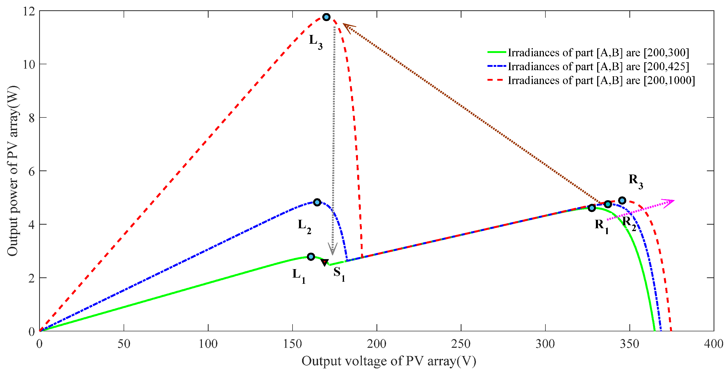
Assuming that the illumination characteristic of the PV array at the moment t is given by the L3–R3 curve, and that the lighting condition changes at moment t + 1, the output characteristic curve of the PV array becomes L1–R1, and the actual PV output becomes S1. As the PV curve exhibits a multi-peak shape, the traditional MPP R1 cannot be obtained by searching the LMPP L1 using the gradient information as in the P & O and INC methods. Some experts found that the overall output power of the PV array changed greatly in this process. Global search algorithms such as the particle swarm optimization (PSO) algorithm or the artificial bee colony (ABC) algorithm can be used for global optimization, by using the amplitudes of the output power variations and the t + 1 global optimal solution R1 to solve the local shadow problems of the PV output characteristics with multiple peaks.

(2)

The light characteristic curve of the PV array is assumed to be the L1–R1 curve at moment t, and the curve of the PV characteristic becomes L3–R3 at moment t + 1, which indicates that the MPP of the PV system should change from R1 to L3.

In this process, as the suboptimal solution R3 of the L3–R3 curve is near R1, the power change is not very large. Therefore, the global search algorithm can be started, which results in the failure of the MPPT algorithm. As can be seen in Figure 4, in this failure case, the power loss ratio is approximately three.

The threshold of the algorithm is inversely proportional to the starting frequency. However, the global optimization search algorithm usually needs a long time to search in an iterative manner, and it is difficult to perform the maximum power search in time when the irradiance changes frequently or continuously.

Therefore, it is difficult to solve the multi-peak problem of local shadowing using the traditional method. The global search algorithm has the problem of slow convergence, and it is difficult to start the global optimization search algorithm using only the current and voltage definitions.

Therefore, it is necessary to use the environment information to make the search judgments, and to utilize fast and efficient tracking algorithms to solve the multi-peak problem of GMPPT under dynamic local shadow conditions.

3. ANN Method for Maximum Power-Point Tracking (MPPT)

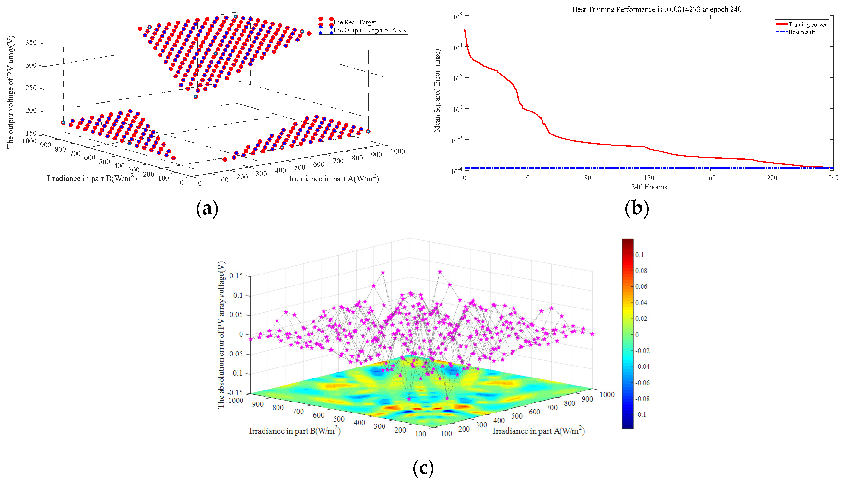
3.1. Neural Network Construction for MPPT

ANNs have recently been developed further, not only in theory but also in practice. A common ANN for MPPT [34,35], showed in Figure 4, has three layers: input, hidden and output layers. In this paper, the ANN input can be the PV-array environmental parameters such as irradiance or temperature and the output is the maximum power. The ANN output is used as the reference power for the DC/DC controller as Formula (4) shows. The input vector x_i in Figure 4a is equal to G_i, which indicates the PV cells’ irradiance for the weights γ_j and λ_ij, while b_j and c are the biases for each joint from the input layer to the output layer.

$$\{\begin{array}{c}{V}_m=\mathsf{\theta }({\displaystyle \sum _{j=1}^m{\mathsf{\gamma }}_j}{\mathsf{\varphi }}_j(G))+c\\ {\mathsf{\varphi }}_j(G)={\mathsf{\rho }}_j({\displaystyle \sum _{i=1}^n({\mathsf{\lambda }}_{ij}}{G}_i+b_j))\end{array}$$

(4)

The training data are determined by using MATLAB/Simulink (R2016b, Mathworks, Natick, MA, USA) to simulate the PV array based on parameters supplied by the manufacturer. For every case, the specific irradiance and temperature values are recorded as the input data to the ANN. The MPP corresponding to each input combination is also recorded as the output data of the ANN. The network is implemented for determining the maximum power of the PV array, when the PV array is subjected to various environmental parameter conditions. The network is obtained through training (supervised) using a training function—the Levenberg–Marquardt algorithm. However, the parameters of a specific PV array have changed over the years; hence, the data used to train the ANN may not be accurate. Therefore, the output reference power is not the exact optimal power. Nevertheless, this reference operation point is close to the MPP.

The DC-DC boost-converter proposed in this paper shows clear advantages over conventional methods, especially under the condition of irradiance mutation.

3.2. Neural Network Analysis for MPPT

In order to show the training result of neural network, according to the irradiance condition in Section 2.3, the regions with the same irradiance are taken as an integrated whole to simplify the structure of the neural network shown in Figure 4a.

According to Figure 5b, it is noted that the output of the PV system varies over time and with the environmental conditions, so the periodic training of the ANN is crucial. A total of 361 sample data points (irradiance between 100 W/m² to 1000 W/m² of part A and B, starting at 100 W/m² in steps of 50 W/m² to 1000 W/m²) were generated to train the network. To perform the ANN, the number of layers, number of neurons of each layer, transmission function of each layer, and kind of training network needs to be assigned. The proposed ANN has three layers; the first and second layers have 10 neurons, while the third layer has one. The first and second layers of the transfer functions are Tansig and the third layer is Purelin. The training data are obtained by simulating the PV system in Matlab/Simulink using the Levenberg–Marquardt algorithm. Two hundred fifty training epochs and applying training as a training function are enough to get good results in Figure 5a. The error computation is performed by algorithm of mean square error method (MSE) during the training process. The admissible of MSE for the ANN is assigned to be approximately 10⁻⁴ in Figure 5b.

Figure 5c shows the changing trend surfaces of the absolution and relative errors at the different irradiances between part A and B. Obviously, in most cases, the absolution errors of ANN output max power are within ±0.15 V. Thus, the results of ANN training are better and are regarded as the reference voltage that is followed by DC/DC converter controller.

4. Topology and Control Strategy for Proposed Power Converter

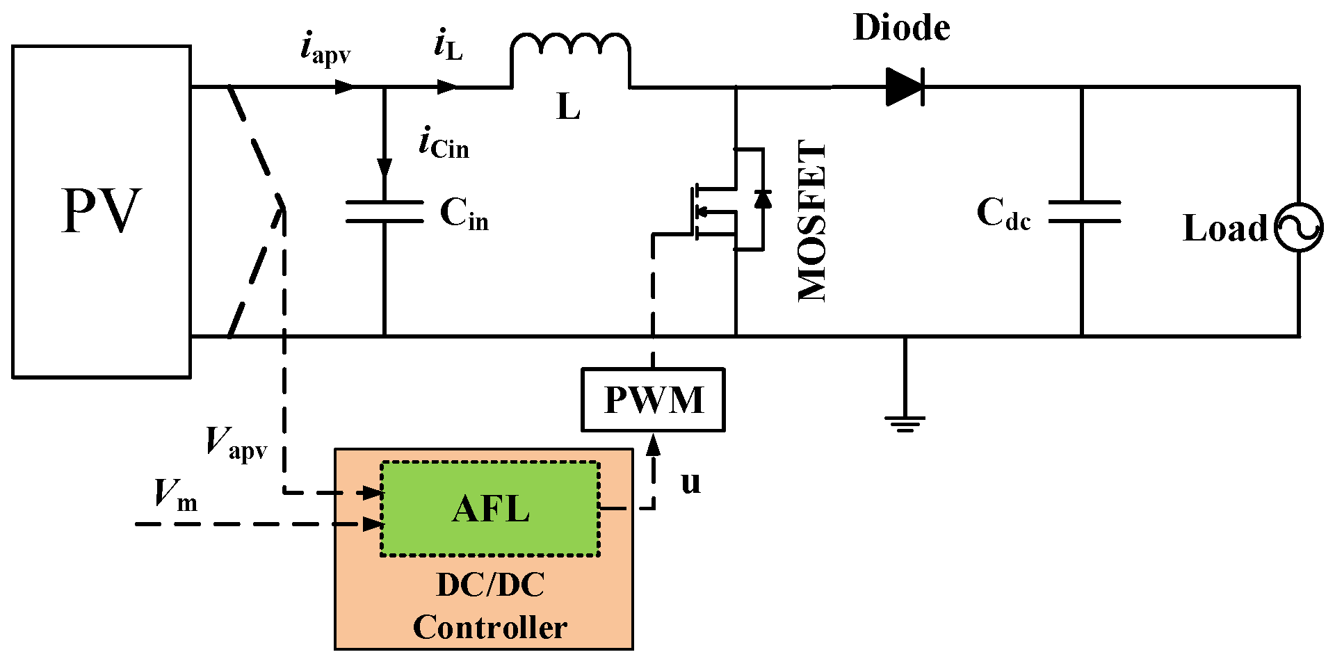
4.1. Nonlinear Model of DC/DC Converter

A simplified circuit scheme of the PV system is presented in Figure 6. The circuit uses a boost converter because of the wide adoption of such a step-up DC/DC structure in PV systems; nevertheless, the analysis presented in this paper can be extended to other DC/DC topologies also. The scheme uses a voltage source as the system load, to model the DC links of double-stage structures in commercial PV inverters where the DC/AC stage regulates the DC-link voltage (C_dc capacitor voltage) [36]. This voltage-source model is widely used to represent the closed-loop grid-connected inverters owing to its satisfactory balance between accuracy and simplicity, which is confirmed in [30,31,32,33,34,35,36,37,38,39,40]. In the topological structure, P_m is the ANN output, namely, the reference power. The control goal of the boost converter is that the actual output power of the PV should be compatible with the P_m of the DC/DC controller.

The dynamic behavior of the DC-DC converter is modeled by the Equations (5) and (6) [41],where i_L represents the inductor current, V_apv is the PV array voltage, I_apv represents the PV array current and P_apv = V_apv × I_apv, V_dc is the DC-link voltage, and L and C_in represent the inductor and capacitor values:

$$\frac{\mathrm{d}{i}_L}{\mathrm{d}t}=\frac{V_{apv}-V_{dc}(1-u)}{L}$$

(5)

$$\frac{\mathrm{d}{V}_{apv}}{\mathrm{d}t}=\frac{I_{apv}-i_L}{C_{in}}.$$

(6)

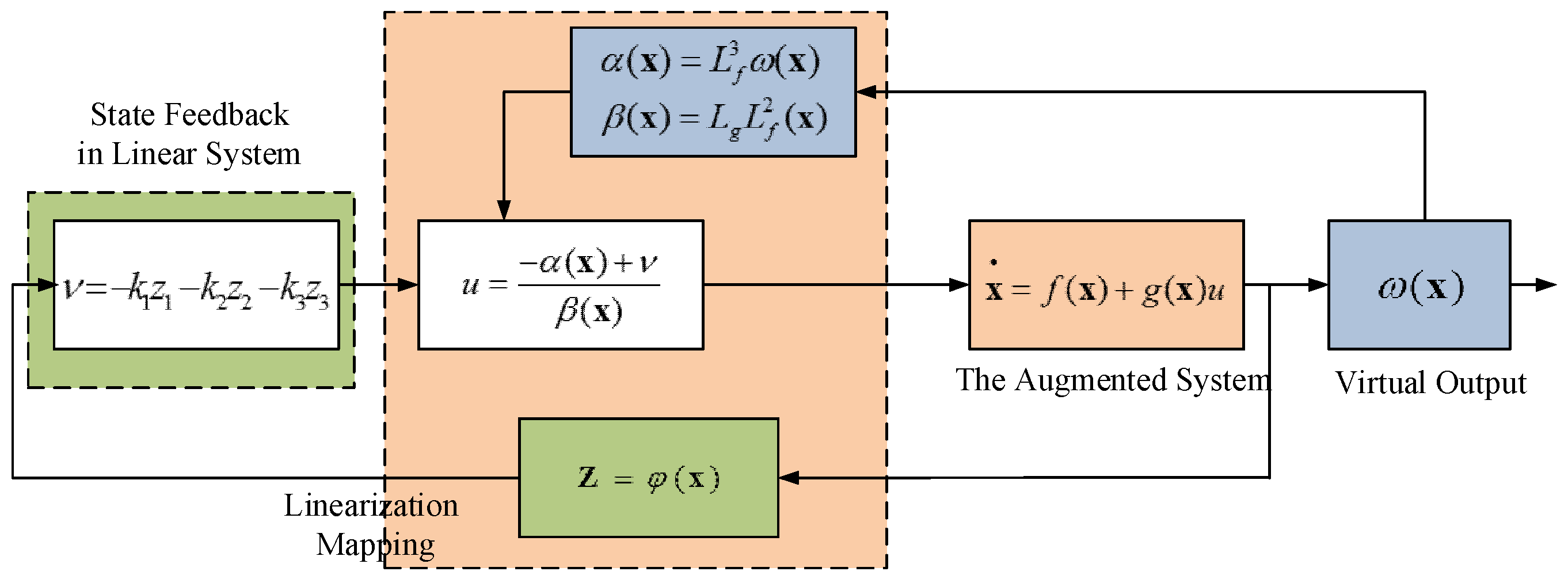
4.2. Augmented-State Feedback Linearization (AFL) Control for Nonlinear Systems

The nonlinear equation system formed by Equations (5) and (6) describes the PV system dynamic behavior under all operating conditions. The traditional PI controller is designed as a linear system. In general, the engineers linearize the nonlinear systems using small-signal modeling methods and adjust the parameters of PI in the linear systems. However, in this method, we need a steady-state point that is to be fixed as the converter working state. In other words, in the fast changing irradiance cases under partial shadow conditions, a linear method such as small-signal modeling cannot satisfy the requirements.

As can be seen from Figure 3, in the PV array under the local shadow conditions there is a significant shift in the static operating point: the voltage at the maximum power point is changed at a large range.

Based on the nonlinear control theory presented in Appendix A, and in conjunction with Equations (2), (3), (5), and (6), we can establish a transformational matrix that varies with time to linearize the nonlinear system under a particular condition [42,43,44]. Then, the state feedback controller is projected onto the linear system to accomplish dynamic tracking. However, the control effect of ordinary state feedback produces steady-state errors.

In order to eliminate the dynamic voltage tracking error under the steady-state condition, a state variable x₃ is defined as x₃ = ∫(V_apv − V_m)dt. The augmented state-space description of the nonlinear system ∑ can be written as follows:

$$\{\begin{array}{l}\stackrel{•}{x_1}=\frac{x_2-V_{dc}}{L}+\frac{V_{dc}}{L}u\\ \stackrel{•}{x_2}=\frac{M(x_2)-x_1}{C_{in}}\\ \stackrel{•}{x_3}=M(x_2)-V_m\end{array},$$

(7)

where the state variable x₁ is the inductor current and x₂ is the capacitor C_in voltage, which is the PV output voltage as well.

The description of ∑ could be written as $\stackrel{•}{x}=f(x)+g(x)u$:

$$f(x)=\left[\begin{array}{l}\frac{x_2-V_{dc}}{L}\\ \frac{M(x_2)-x_1}{C_{in}}\\ M(x_2)-V_m\end{array}\right],g(x)=\left[\begin{array}{l}\frac{V_{dc}}{L}\\ 0\\ 0\end{array}\right].$$

According to the nonlinear control theory and definitions mentioned in Appendix A, the augmented system ∑ could be partially feedback linearized by constructing a considered output function. Assuming the output function $y=\mathsf{\omega }(x)$, the criteria ${\mathrm{L}}_g\mathsf{\omega }(x)=0$, ${\mathrm{L}}_g{\mathrm{L}}_f\mathsf{\omega }(x)=0$ and ${\mathrm{L}}_g{{\mathrm{L}}^2}_f\mathsf{\omega }(x)\ne 0$ should be met.

By analyzing the characteristic of control matrix $g(x)$, the criteria could be met when the output function is considered as $\mathsf{\omega }(x)=x_3$. A new state variable Z could be defined as $Z=\mathsf{\phi }(x)={[\mathsf{\omega }(x),{\mathrm{L}}_f\mathsf{\omega }(x),{{\mathrm{L}}^2}_f\mathsf{\omega }(x)]}^{\mathrm{T}}$ to construct a coordinate transformation.

The augmented system ∑ could be mapped to a third-order linear time-invariant system Π as follows:

$$\stackrel{•}{Z}=\left[\begin{array}{ccc}0& 1& 0\\ 0& 0& 1\\ 0& 0& 0\end{array}\right]Z+\left[\begin{array}{c}0\\ 0\\ 1\end{array}\right]\mathsf{\nu },$$

(8)

where $\mathsf{\nu }$ is the controlled variable in system Π.

The controlled variable u in system ∑ can be written as:

$$u=\frac{-{{\mathrm{L}}^3}_f\mathsf{\omega }(x)+\mathsf{\nu }}{{\mathrm{L}}_g{{\mathrm{L}}^2}_f\mathsf{\omega }(x)}.$$

(9)

From Equation (9), it can be seen that the controlled variables in system ∑ could be described by the controlled variable ν in the third-order linear time-invariant system Π. The response curve of system ∑ is determined by the controlled variable ν.

The control law $\mathsf{\nu }=-KZ=-k_1{z}_1-k_2{z}_2-k_3{z}_3$ could be designed according to the theory of linear system, then, substituting it into Equation (8), it could be written as Equation (10):

$$\stackrel{••}{z_1}+k_3\stackrel{•}{z_1}+k_2{z}_1+k_1{\displaystyle \int z_1\mathrm{d}t}=0,$$

(10)

where $z_1=\mathsf{\omega }(x)=x_3={\displaystyle \int (V_{pv}-V_{mpp})\mathrm{d}t}$.

The state variable $z_1$ is determined by feedback coefficient matrix $K=[k_1,k_2,k_3]$ in the third-order differential equation, and the effect of PV output voltage V_apv given by ANN tracking reference V_m is determined as well.

A third-order system could be considered as a product of a first-order system and a second-order system. The system can be reduced to a reasonable order according to the system distribution of the roots, which means by designing the dominant pole placement. The system is designed as a second-order system in this paper, that is, the distance between the roots and the imaginary axis in the first-order system is larger than three times the distance between the roots and the imaginary axis in the second-order system. The state variables $z_{1,1}$, $z_{1,2}$, and $z_{1,3}$could be written as $z_{1,1}={\mathsf{\omega }}_n$, $z_{1,2}=-\mathsf{\xi }{\mathsf{\omega }}_n+{\mathsf{\omega }}_n\sqrt{{\mathsf{\xi }}^2-1}$, and $z_{1,3}=-\mathsf{\xi }{\mathsf{\omega }}_n-{\mathsf{\omega }}_n\sqrt{{\mathsf{\xi }}^2-1}$. $\mathsf{\xi }$ is the second-order system damping ratio that affects the system dynamic performance. In order to be an overdamped system, ξ should be greater than or equal to 3. ${\mathsf{\omega }}_n$ is the system natural frequency that affects the steady-state precision and corresponding velocity, and ${\mathsf{\omega }}_n$ is supposed to be k times the LC_in circuit resonant frequency. The control parameters of the system could be written as (11):

$$\{\begin{array}{c}{k}_1={\mathsf{\omega }}_n^3=k{(1/\sqrt{L{C}_{in}})}^3\\ k_2=(2\mathsf{\xi }+1){\mathsf{\omega }}_n^2\\ k_3=(2\mathsf{\xi }+1){\mathsf{\omega }}_n\end{array}.$$

(11)

The augmented state-space feedback linearization control strategy is presented in Figure 7.

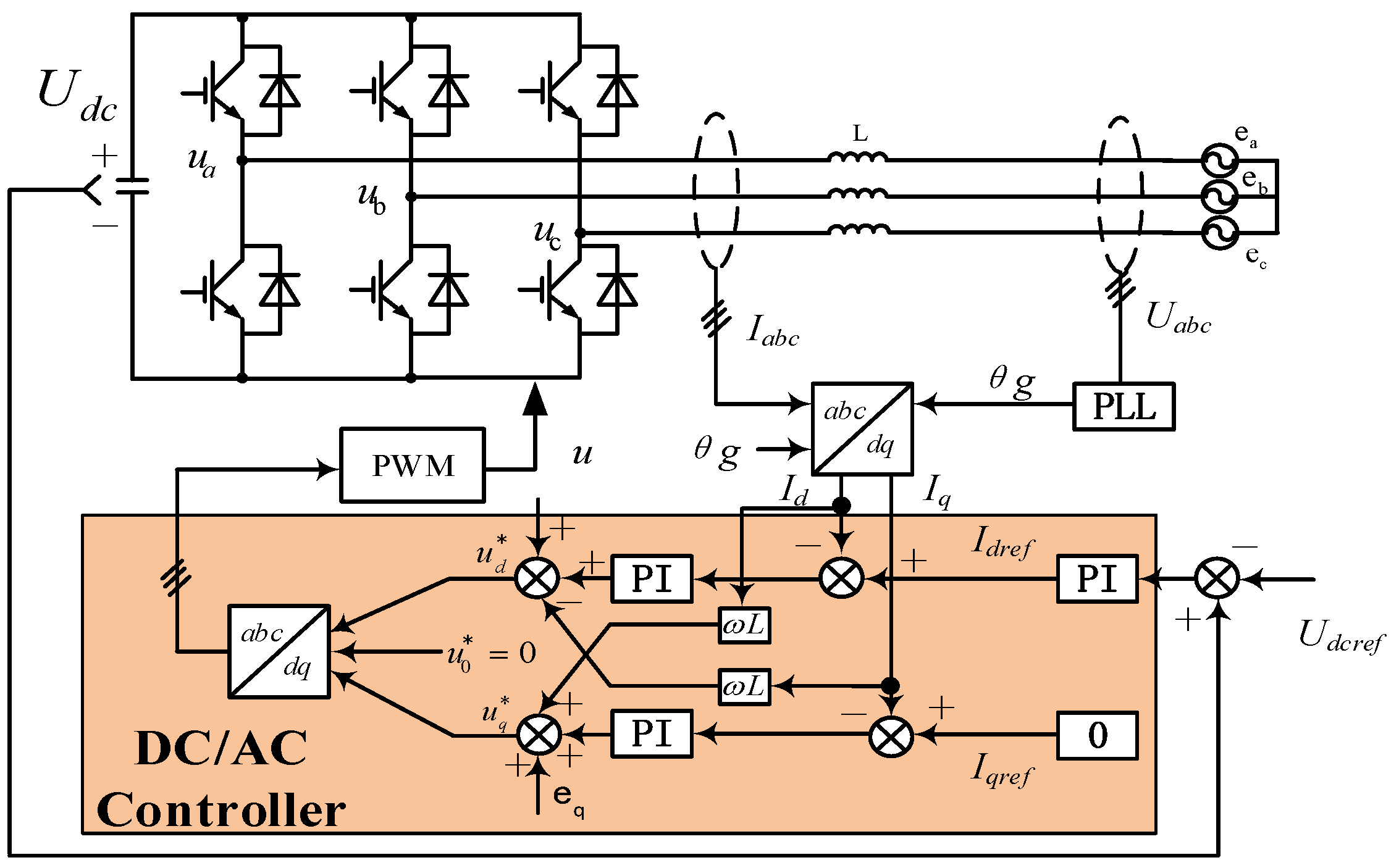
4.3. DC/AC Inverter and Control

Figure 8 shows a typical topology of a two-stage grid-connected PV system, which includes a DC/DC boost converter and a DC/AC converter. The first-stage DC/DC boost converter connected to the PV panel steps up the output DC voltage of the DC bus to a level appropriate for the DC/AC inverter, based on the MPPT algorithm.

The DC/AC inverter control strategy is based on the instantaneous powers of the d–q frame references applied for pulse-width modulation (PWM) control. According to the instantaneous power theory, the active power p and reactive power q can be written as in Equation (10):

$$\{\begin{array}{l}p=\frac{3}{2}(e_d{i}_d+e_q{i}_q)\\ q=\frac{3}{2}(e_d{i}_q-e_q{i}_d)\end{array},$$

(12)

where $e_d$, $e_q$, $i_d$, and $i_q$ are d–q components of the grid voltage and d–q components of the output current, respectively. $\left|E\right|$ is the amplitude of the grid voltage. On the d–q frame references under the voltage-oriented control (V_OC) method, $e_d=\left|E\right|$, $e_q=0$. Thus,

$$\{\begin{array}{l}p=\frac{3}{2}{e}_d{i}_d\\ q=\frac{3}{2}{e}_d{i}_q\end{array}.$$

(13)

Ignoring the inverter attenuation losses, the instantaneous value of the DC-link power p_dc can be described as shown in Equation (14):

$$p_{dc}=i_{dc}{u}_{dc}.$$

(14)

The active power p and p_dc could be represented as

$$i_{dc}{u}_{dc}=p=\frac{3}{2}{e}_d{i}_d.$$

(15)

The control scheme of the grid-side inverter is shown in Figure 8. The internal d–q current loop references can be calculated from the external loop, and the PI controller is used to regulate the d–q grid currents [45,46,47]. The outputs of the d–q current controllers, ΔV_gd and ΔV_gq, which denote a variation of the grid voltage, are added to the d–q grid voltages to obtain the dynamic response with the feedforward of the grid voltage [48]. In order to operate in terms of unity power factor with grid, I_qref is set to 0.

5. Digital Simulation Experiments and Analysis

5.1. Simulation Case 1

The purpose of testing the rapidity and effectiveness of tracking the MPP voltage of PV arrays under PSC is to verify the GMPPT nonlinear control method proposed in simulation case 1.

The performance of the proposed MPPT method based on nonlinear control is evaluated under conditions where the irradiance changes rapidly, by using Matlab/Simulink. The PV array model proposed in this paper is shown in Figure 2b, where N_s = 6, N_p = 12, and N_s1 = 3 is region A, and N_s2 = 3 is shown as area B. The parameters of the solar module are presented in Table 1. The irradiances of regions A and B are shown in Figure 9. The simulation parameters are presented in Appendix B, and the simulation results are shown in Figure 9, Figure 10, Figure 11, Figure 12, Figure 13 and Figure 14.

The peaks under 200 V in Figure 9 are defined as the left peaks and the peaks above 200 V are defined as the right peaks.

It can be seen from Figure 9 that during the simulation the irradiance can change gradually or abruptly. The amplitude of the MPP voltage also deviates frequently by more than 150 V; that is, the MPP keeps moving between the left and right peaks with changes in irradiance. The MPP is on the right peak in area a of Figure 9A. As the irradiance increases, the MPP moves to the left peak at 0.16 s and keeps increasing, as shown in Figure 9B. At 0.35 s, the MPP is still on the left peak when the irradiance decreases from 1000 W/m² to 550 W/m² suddenly. At 0.4 s, the MPP on the left peak shifts to the right peak when the irradiance decreases from 550 W/m² to 250 W/m², as shown in area d of Figure 9A. At 0.45 s, 0.5 s, 0.55 s, and 0.74 s, the irradiance changes as shown in Figure 9a, accompanied by a shift of the MPP from the left peak to the right peak.

In order to verify the method proposed in this paper, the simulation conditions are designed to simulate a variety of changes in the PV array. The simulation conditions are consistent with the analysis in Section 2.3.

It can be observed from Figure 10 that, in areas a, b, c, e, g, and h, the AFL method can track the MPP voltage quickly and without steady-state errors, under conditions where the irradiance changes slowly or rapidly; this is obviously superior to the FL method.

In areas (A) to (B) and stages d–h, even if the MPP voltage changes in a wide range and the dynamic tracking process produces a large overshoot, the controller can still respond within 0.03 s to the new voltage reference. As can be observed in Figure 10, the AFL method can track the MPP voltage quickly, accurately, and statically.

At the same time, the hybrid control method (ANN + AFL) proposed in this paper can achieve MPPT and eliminate the possibility of GMPPT failures, regardless of the changes in the PV shielding conditions.

The control effect of MPPT focuses on the output power of the PV system, as shown in Figure 11. It can be seen from Figure 11 that the AFL controller can realize the MPP with high efficiency and can accurately track the MPP voltage.

Although the transients in the PV output current cause a power surge at the point of MPP voltage mutation, especially in the case of a wide range of mutations, the AFL controller eliminates the dynamic processes in a short period and stabilizes the output power.

It can be seen from Figure 11 and Figure 12 that in parts a, d, e, and h of the simulation process, which indicate MPP in the right peaks, the currents in regions A and B are equal because of low irradiances.

As regions A and B of different lighting conditions result in different MPP voltages, the PV array output power comes from regions A and B together.

In the simulation process of b, c, f, and g, the irradiance of region B is much higher than that of region A, and the output power of region B is larger than the sum of the powers of regions A and B.

Therefore, the bypass diode of region A turns on, and the region A voltage is clamped by the diode conduction voltage. At this time, the PV output voltages and powers generated by the region B from 0.16 s to 0.4 s and from 0.5 s to 0.74 s are shown in Figure 13.

The DC-link voltage and the output current of the PV grid-connected inverter are depicted in Figure 13a. It can be observed that the DC-link voltage is maintained at 700 V and that the fluctuations are within an acceptable range of approximately 15 V.

The effectiveness of the hybrid MPPT method presented in this paper is shown in Figure 13b. The output current is consistent with the PV output characteristic curve in Figure 9a.

5.2. Simulation Case 2

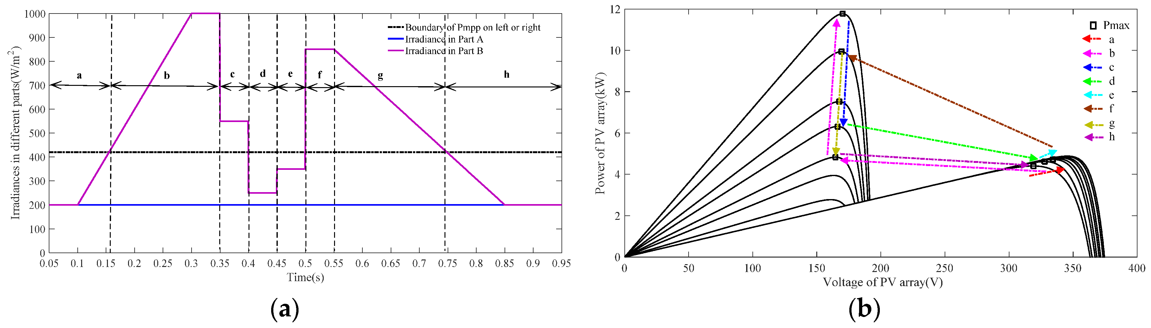
In this case, simulations are carried out under different scenarios to compare the proposed MPPT method with other methods such as the conventional P & O method [5] and the improved P & O method [4]. The duration of simulation is 2 s, which is separated into three sections as illustrated in

Table 2. Considered shading conditions.

Section No.	Time (s)	Shading Pattern [G1,1~12, G2,1~12, G3,1~12, G4,1~12, G5,1~12, G6,1~12] (W/m2)
SP1	0.1~0.3	[300, 300, 300, 1000, 700, 700]
SP2	0.3~1.5	[300, 300, 300, 1000, 500, 500]
SP3	1.5~2.0	[300, 300, 300, 1000, 1000, 300]

.

From Table 2 and Figure 14, it can be observed that the simulation process consists of three different partial shading processes. It is assumed that under the simulation pattern 1 (SP1), all three methods can achieve MPP.

(1)

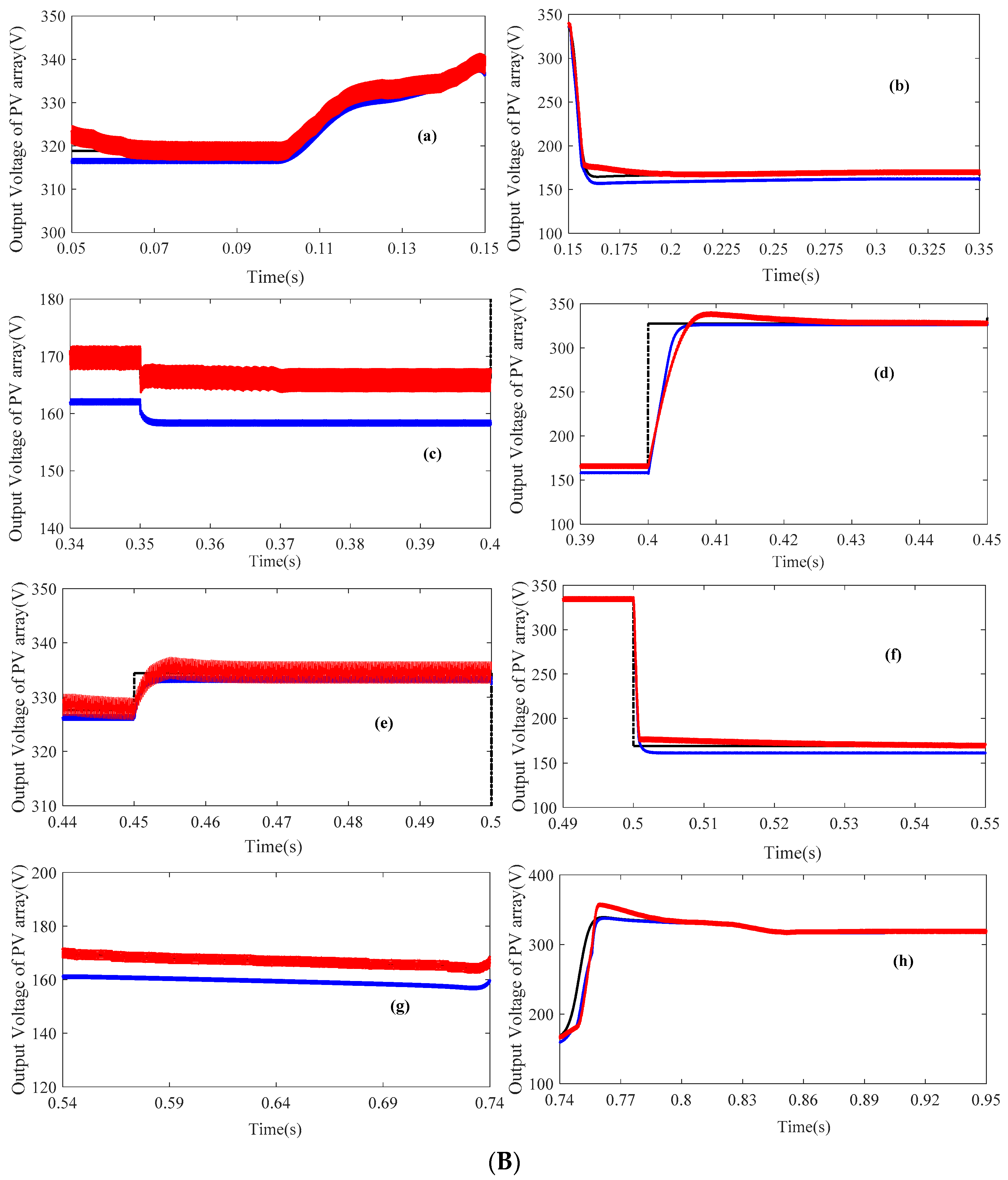
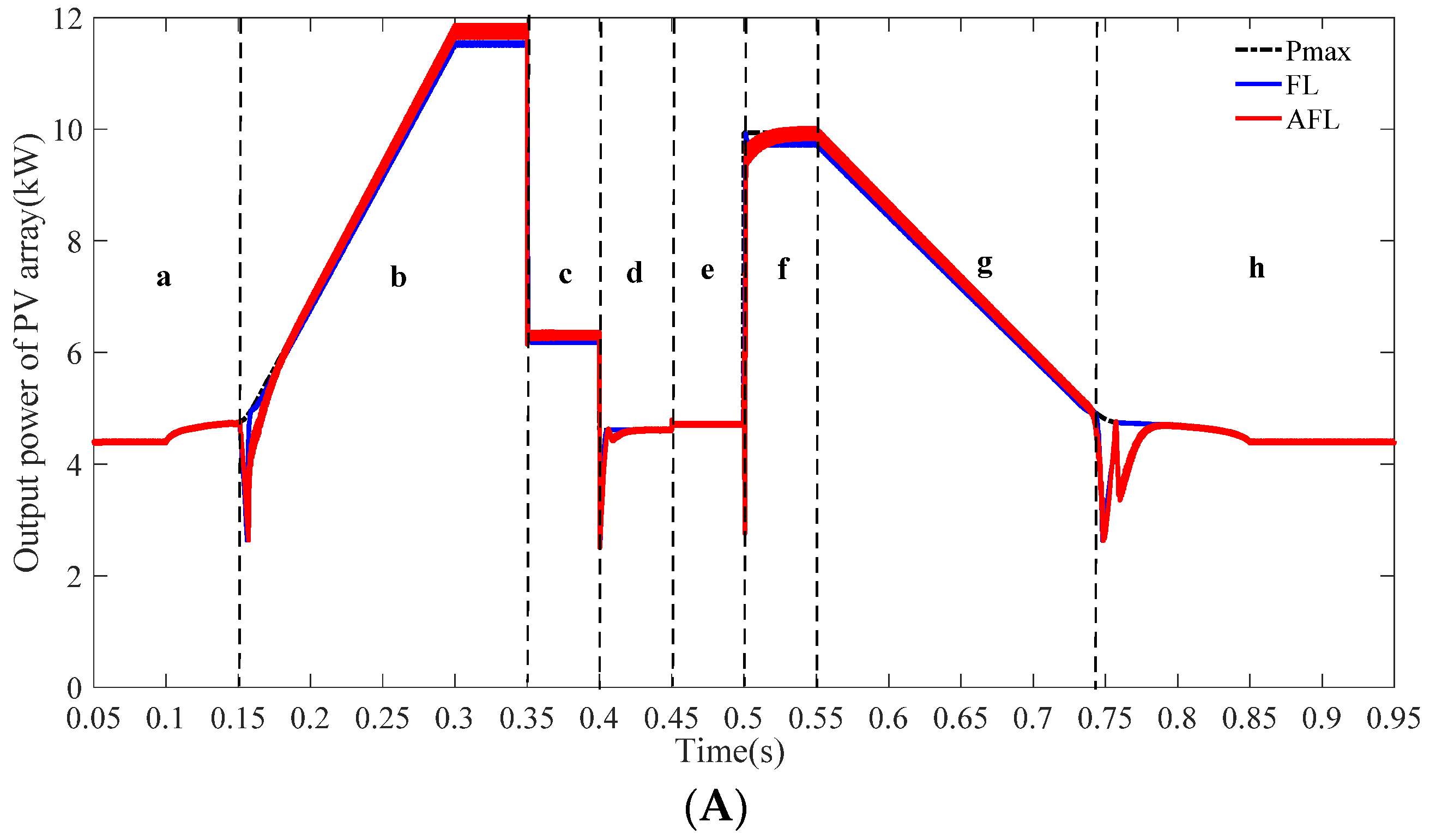
As shown in Part I of Figure 14, when the shading condition changes to SP2 from SP1, the PV output characteristic changes from the pink curve to the brown curve. The traditional P & O algorithm (the green curve in Figure 14) can track the MPP (point a) in section SP1. However, only the local MPP (point b) in section SP2 can be tracked by the traditional P & O algorithm, which indicates that the traditional P & O algorithm for MPPT fails to track the GMPP in section SP2. Since the instantaneous power change ΔP is large, the improved P & O algorithm (the blue curve in Figure 14) can start the global search module and track the GMPP (point c), similar to the method proposed in this paper (the red curve in Figure 14). It is clear from the dynamic process that the response time of the proposed method is much less than that of the improved P & O algorithm, and that the tracking speed is increased more than 6-fold. By combining this inference with the information in

Table 3. Performances of the different MPPT (maximum power point tracking) methods under different scenarios.

Section No.	Ideal Maximum Power (W)	Output Power Obtained (W)
		P & O	Improved P & O	ANN + AFL 1
SP1	8393.4	8282.9	8283.1	8381.4
SP2	7341.3	5989.2	7225.3	7311.2
SP3	7811.6	7108.4	7112.6	7798.8

¹ ANN: artificial neural network; AFL: augmented state feedback precise linearization.

, it can be inferred that the steady-state maximum power of the proposed method is also superior to that of the improved P & O algorithm.

(2)

When the shading condition changes to SP2 from SP3, the PV output characteristic changes from the brown curve to the black curve, as shown in Figure 14II. It can be seen that the MPP (point c) of the SP2 shading condition is near the local MPP (point d) of the SP3 shading condition. It is difficult to start the global search because the power change due to the shading condition change is not large enough. Therefore, the improved P & O and traditional P & O algorithms track the local MPP (point d) in identical manners, which indicates that the GMPP tracking fails in the cases of the improved P & O and traditional P & O algorithms. It can be seen from Table 3 that the power loss caused by MPPT failure is 699 W, which accounts for approximately 10% of the maximum power. The method proposed in this paper can track the MPP (point e) quickly and accurately, and effectively solve the MPPT failure problem caused by local shadow conditions.

6. Conclusions

Control methods for MPPT and for the entire grid-connected PV power generation system under PSC were proposed in this paper. An ANN was combined with the nonlinear controller of a DC/DC converter to obtain good tracking, especially in case of fast irradiance changes. Under the simulation conditions discussed in the paper, the following conclusions could be drawn:

(1)

The PV output characteristics were modeled and analyzed under PSC, and the complex nonlinear multi-peak morphology of the PV array output was verified. It was found that the timings of irradiance changes might cause the failure of traditional MPPT methods or make it difficult to define the starting conditions, especially for MPPT algorithms based on voltage or current information.

(2)

Based on the above analysis, an artificial neural training network model was designed based on environmental variables and irradiance information, and GMPPT was realized efficiently and effectively using the hybrid method (ANN + AFL) for the DC/DC converter. A comparison of the proposed MPPT method with the conventional P & O method and the improved P & O method was illustrated through simulations. The GMPPT failure caused by the timing of the irradiance change was solved.

(3)

For the problems caused by the partial shading process, such as the MPP voltage of the PV output being shifted greatly, the static operating point of the system being changed, or the difficulty of designing a PI controller to eliminate the steady state under small-signal modeling, this paper proposed an AFL control method for nonlinear systems to accurately track the MPP without static errors. The control parameters were clear and easy to design and apply.

References

1. Mathiesen, B.V.; Lund, H.; Karlsson, K. 100% renewable energy systems, climate mitigation and economic growth. Appl. Energy 2011, 88, 488–501. [Google Scholar] [CrossRef]
2. Carcangiu, G.; Dainese, C.; Faranda, R.; Leva, S.; Sardo, M. New network topologies for large scale photovoltaic systems. In Proceedings of the IEEE Power Tech Conference 2009, Bucharest, Romania, 28 June–2 July 2009; pp. 1–7.
3. Mamarelis, E.; Petrone, G.; Spagnuolo, G. A two-steps algorithm improving the P & O steady state MPPT efficiency. Appl. Energy 2014, 113, 414–421. [Google Scholar]
4. Hiren, P.; Vivek, A. Maximum Power Point Tracking Scheme for PV Systems Operating Under Partially Shaded Conditions. IEEE Trans. Power Electron. 2008, 55, 1689–1698. [Google Scholar]
5. Nicola, F.; Giovanni, P.; Giovanni, S.; Massimo, V. Optimization of perturb and observe maximum power point tracking method. IEEE Trans. Power Electron. 2005, 20, 963–973. [Google Scholar]
6. Qiang, M.; Mingwei, S.; Liying, L.; Guerrero, J.M. A Novel Improved Variable Step-Size Incremental-Resistance MPPT Method for PV Systems. IEEE Trans. Ind. Electron. 2011, 58, 2427–2434. [Google Scholar]
7. Alberto, D.; George, C.L.; Sonia, L.; Giampaolo, M. Experimental investigation of partial shading scenarios on PV (photovoltaic) modules. Energy 2013, 55, 466–475. [Google Scholar]
8. Singh, M.D.; Shine, V.J.; Janamala, V. Application of artificial neural networks in optimizing MPPT control for standalone solar PV system. In Proceedings of the 2014 International Conference on Contemporary Computing and Informatics (IC3I), Mysore, India, 27–29 November 2014; pp. 162–166.
9. Faranda, R.; Leva, S.; Maugeri, V. MPPT techniques for PV systems: Energetic and cost comparison. In Proceedings of the IEEE Power and Energy Society 2008 General Meeting, Pittsburgh, PA, USA, 20–24 July 2008.
10. Berrera, M.; Dolara, A.; Faranda, R.; Leva, S. Experimental test of seven widely-adopted MPPT algorithms. In Proceedings of the 2009 IEEE Bucharest PowerTech: Innovative Ideas Toward the Electrical Grid of the Future, Bucharest, Romania, 28 June–2 July 2009.
11. Martınez-Moreno, F.; Munoz, J.; Lorenzo, E. Experimental model to estimate shading losses on PV arrays. J. Sol. Energy Mater. Sol. Cells 2010, 94, 2298–2303. [Google Scholar] [CrossRef] [Green Version]
12. Yazdani, A.; Di Fazio, A.R.; Ghoddami, H.; Russo, M.; Kazerani, M.; Jatskevich, J.; Strunz, K.; Leva, S.; Martinez, J.A. Modeling guidelines and a benchmark for power system simulation studies of three-phase single stage photovoltaic systems. IEEE Trans. Power Deliv. 2011, 26, 1247–1264. [Google Scholar] [CrossRef]
13. Potnuru, S.R.; Pattabiraman, D.; Ganesan, S.I.; Chilakapati, N. Positioning of PV panels for reduction in line losses and mismatch losses in PV array. Renew. Energy 2015, 78, 264–275. [Google Scholar] [CrossRef]
14. Sahu, H.S.; Nayak, S.K.; Mishra, S. Maximizing the Power Generation of a Partially Shaded PV Array. IEEE J. Emerg. Sel. Top. Power Electron. 2016, 4, 626–637. [Google Scholar] [CrossRef]
15. Patel, H.; Agarwal, V. MATLAB-Based Modeling to Study the Effects of Partial Shading on PV Array Characteristics. IEEE Trans. Energy Convers. 2008, 23, 302–310. [Google Scholar] [CrossRef]
16. Liu, X.; Qi, X.; Zheng, S.; Wang, F.; Chen, D. Model and Analysis of Photovoltaic Array under Partial Shading. Power Syst. Technol. 2010, 34, 192–197. [Google Scholar]
17. Dıaz-Dorado, E.; Cidras, J.; Carrillo, C. Discrete I–V model for partially shaded PV-arrays. Sol. Energy 2014, 103, 96–107. [Google Scholar] [CrossRef]
18. Alberto, D.; Sonia, L.; Manzolini, G. Comparison of different physical models for PV power output prediction. Sol. Energy 2015, 119, 83–99. [Google Scholar] [Green Version]
19. Kadri, R.; Andrei, H.; Gaubert, J.-P. Modeling of the photovoltaic cell circuit parameters for optimum connection model and real-time emulator with partial shadow conditions. Energy 2012, 42, 57–67. [Google Scholar] [CrossRef]
20. Ahmed, J.; Salam, Z. An Improved Method to Predict the Position of Maximum Power Point during Partial Shading for PV Arrays. IEEE Trans. Ind. Inform. 2015, 11, 1378–1387. [Google Scholar] [CrossRef]
21. Ji, Y.-K.; Jung, D.-Y.; Kim, J.-G.; Kim, J.-H.; Lee, T.-W.; Won, C.-Y. A Real Maximum Power Point Tracking Method for Mismatching Compensation in PV Array under Partially Shaded Conditions. IEEE Trans. Power Electron. 2011, 26, 1001–1009. [Google Scholar] [CrossRef]
22. Murtaza, S.; Chiaberge, M.; Spertino, F.; Boero, D.; De Giuseppe, M. A maximum power point tracking technique based on bypass diode mechanism for PV arrays under partial shading. Energy Build. 2014, 73, 13–25. [Google Scholar] [CrossRef]
23. Sundareswaran, K.; Vignesh kumar, V.; Palani, S. Application of a combined particle swarm optimization and perturb and observe method for MPPT in PV systems under partial shading conditions. Renew. Energy 2015, 75, 308–317. [Google Scholar] [CrossRef]
24. Hajighorbani, S.; Radzi, M.A.M.; Ab Kadir, M.Z.A.; Shafie, S.; Zainuri, M.A.A.M. Implementing a Novel Hybrid Maximum Power Point Tracking Technique in DSP via Simulink/MATLAB under Partially Shaded Conditions. Energies 2016, 9, 1–25. [Google Scholar] [CrossRef]
25. Ghasemi, M.A.; Forushani, H.M.; Parniani, M. Partial Shading Detection and Smooth Maximum Power Point Tracking of PV Arrays Under PSC. IEEE Trans. Power Electron. 2016, 31, 6281–6292. [Google Scholar] [CrossRef]
26. Liu, T.-H.; Chen, J.-H.; Huang, J.-W. Global maximum power point tracking algorithm for PV systems operating under partially shaded conditions using the segmentation search method. Sol. Energy 2014, 103, 350–363. [Google Scholar] [CrossRef]
27. Lyden, S.; Haque, M.E. A Simulated Annealing Global Maximum Power Point Tracking Approach for PV Modules Under Partial Shading Conditions. IEEE Trans. Power Electron. 2016, 31, 4171–4181. [Google Scholar] [CrossRef]
28. Ahmed, J.; Salam, Z. A Maximum Power Point Tracking (MPPT) for PV system using Cuckoo Search with partial shading capability. Appl. Energy 2014, 119, 118–130. [Google Scholar] [CrossRef]
29. Syafaruddin; Karatepe, E.; Hiyama, T. Artificial neural network-polar coordinated fuzzy controller based maximum power point tracking control under partially shaded conditions. IET Renew. Power Gener. 2009, 3, 239–253. [Google Scholar] [CrossRef]
30. Rizzo, S.A.; Scelba, G. ANN based MPPT method for rapidly variable shading conditions. Appl. Energy 2015, 145, 124–132. [Google Scholar] [CrossRef]
31. Liu, Y.-H.; Huang, S.-C.; Huang, J.-W.; Liang, W.-C. A Particle Swarm Optimization-Based Maximum Power Point Tracking Algorithm for PV Systems Operating Under Partially Shaded Conditions. IEEE Trans. Energy Convers. 2012, 27, 1027–1035. [Google Scholar] [CrossRef]
32. Mohanty, S.; Subudhi, B.; Ray, P.K. A New MPPT Design Using Grey Wolf Optimization Technique for Photovoltaic System under Partial Shading Conditions. IEEE Trans. Sustain. Energy 2016, 7, 181–188. [Google Scholar] [CrossRef]
33. Benyoucef, A.S.; Chouder, A.; Kara, K. Artificial bee colony based algorithm for maximum power point tracking (MPPT) for PV systems operating under partial shaded conditions. Appl. Soft Comput. 2015, 32, 38–48. [Google Scholar] [CrossRef]
34. Jiang, L.L.; Nayanasiri, D.R.; Maskell, D.L.; Vilathgamuwa, D.M. A hybrid maximum power point tracking for partially shaded photovoltaic systems in the tropics. Renew. Energy 2015, 76, 53–65. [Google Scholar] [CrossRef]
35. Elobaid, L.M.; Abdelsalam, A.K.; Zakzouk, E.E. Artificial neural network-based photovoltaic maximum power point tracking techniques: A survey. IET Renew. Power Gener. 2015, 9, 1043–1063. [Google Scholar] [CrossRef]
36. Trejos, A.; Gonzalez, D.; Ramos-Paja, C.A. Modeling of Step-up Grid-Connected Photovoltaic Systems for Control Purposes. Energies 2012, 5, 1900–1926. [Google Scholar] [CrossRef]
37. Manganiello, P.; Ricco, M.; Petrone, G.; Monmasson, E.; Spagnuolo, G. Optimization of Perturbative PV MPPT Methods through Online System Identification. IEEE Trans. Ind. Electron. 2014, 61, 6812–6821. [Google Scholar] [CrossRef]
38. Renaudineau, H.; Donatantonio, F.; Fontchastagner, J.; Petrone, G.; Spagnuolo, G.; Martin, J.-P.; Pierfederici, S. A PSO-Based Global MPPT Technique for Distributed PV Power Generation. IEEE Trans. Ind. Electron. 2015, 62, 1047–1058. [Google Scholar] [CrossRef]
39. Mamarelis, E.; Petrone, G.; Spagnuolo, G. An Hybrid Digital-Analog Sliding Mode Controller for Photovoltaic Applications. IEEE Trans. Ind. Inf. 2103, 9, 1094–1103. [Google Scholar] [CrossRef]
40. Haroun, R.; Aroudi, A.E.; Cid-Pastor, A.; Garcia, G.; Olalla, C.; Martinez-Salamero, L. Impedance Matching in Photovoltaic Systems Using Cascaded Boost Converters and Sliding-Mode Control. IEEE Trans. Power Electron. 2015, 30, 3185–3199. [Google Scholar] [CrossRef]
41. Erickson, R.W.; Maksimovic, D. Fundamentals of Power Electronics, 2nd ed.; Springer: Berlin, Germany, 2007. [Google Scholar]
42. Abbasi, M.H.; Moradian, H. Improving the performance of a nonlinear boiler-turbine unit via bifurcation control of external disturbances: A comparison between sliding mode and feedback linearization control approaches. Nonlinear Dyn. 2016, 85, 229–243. [Google Scholar]
43. Ding, X.; Sinha, A. Hydropower Plant Frequency Control Via Feedback Linearization and Sliding Mode Control. J. Dyn. Syst. Meas. Control-Trans. ASME 2016, 138, 074501. [Google Scholar] [CrossRef]
44. Alonge, F.; Cirrincione, M.; Pucci, M.; Sferlazza, A. Input- Output Feedback Linearization Control with On-Line MRAS-Based Inductor Resistance Estimation of Linear Induction Motors Including the Dynamic End Effects. IEEE Trans. Ind. Appl. 2016, 52, 254–266. [Google Scholar] [CrossRef]
45. Dannehl, J.; Wessels, C.; Fuchs, F.W. Limitation of voltage-oriented PI current control of grid-connected PWM rectifier with LCL filters. IEEE Trans. Ind. Electron. 2009, 56, 380–388. [Google Scholar] [CrossRef]
46. Dannehl, J.; Fuchs, F.W.; Hansen, S.; Thogersen, P.B. Investigation of active damping approaches for PI-based current control of grid-connected pulse width modulation converter with LCL filters. IEEE Trans. Ind. Appl. 2010, 46, 1509–1517. [Google Scholar] [CrossRef]
47. Dannehl, J.; Fuchs, F.W.; Thogersen, P.B. PI state current control of grid-connected PWM converters with LCL filters. IEEE Trans. Power Electron. 2010, 25, 2320–2330. [Google Scholar] [CrossRef]
48. Hwang, T.S.; Park, S.Y. A seamless control strategy of a distributed generation inverter for the critical load safety under strict grid disturbances. IEEE Trans. Power Electron. 2013, 28, 4780–4790. [Google Scholar] [CrossRef]
Figure 1. Structure of a PV (photovoltaic) system with a classical MPPT (maximum power point tracking)-based ANN (artificial neural network).
Applsci 07 00095 g001
Figure 2. Schematic model of PV array: (a) PV substring under shading condition; (b) V–I characteristic curve corresponding to (a); (c) PV array model.
Applsci 07 00095 g002
Figure 3. V–P characteristics of PV array under PSC (maximum power point).
Applsci 07 00095 g003
Figure 4. Structure of ANN in MPPT: (a) Typical ANN structure; (b) ANN structure proposed in this paper.
Applsci 07 00095 g004
Figure 5. Testing data of ANN controller: (a) The output of the neural network training with the amount of target data; (b) the mean squared error (MSE) in converging process; (c) the absolute error of neural network training.
Applsci 07 00095 g005
Figure 6. Topology of DC-DC boost converter in PV system.
Applsci 07 00095 g006
Figure 7. Augmented state-space feedback linearization control strategy.
Applsci 07 00095 g007
Figure 8. Control strategy of DC/AC inverter.
Applsci 07 00095 g008
Figure 9. (a) Irradiances of different parts of the PV array; (b) voltage of the PV array.
Applsci 07 00095 g009
Figure 10. Output voltage of PV systems with AFL (augmented state feedback precise linearization) and FL (state feedback precise linearization) controller: (A) Output voltage (overall); (B) output voltage (detailed): (a) output voltage (0.05–0.15 s); (b) output voltage (0.15–0.35 s); (c) output voltage (0.35–0.40 s); (d) output voltage (0.40–0.45 s); (e) output voltage (0.45–0.50 s); (f) output voltage (0.50–0.55 s); (g) output voltage (0.55–0.74 s); (h) output voltage (0.74–0.95 s).
Applsci 07 00095 g010aApplsci 07 00095 g010b
Figure 11. Output power of PV systems with AFL and FL: (A) Output power (overall); (B) output power (detailed): (a) output power (0.05–0.15 s); (b) output power (0.15–0.35 s); (c) output power (0.35–0.40 s); (d) output power (0.40–0.45 s); (e) output power (0.45–0.50 s); (f) output power (0.50–0.55 s); (g) output power (0.55–0.74 s); (h) output power (0.74–0.95 s).
Applsci 07 00095 g011aApplsci 07 00095 g011b
Figure 12. Output current and voltage in different parts of the PV array.
Applsci 07 00095 g012
Figure 13. DC-link voltage and inverter output current: (a) DC-link voltage; (b) three-phase output current.
Applsci 07 00095 g013
Figure 14. Comparison of proposed MPPT method with the P & O (perturb and observe) and improved P & O methods, under different scenarios.
Applsci 07 00095 g014