ℓ_2,1 Norm and Hessian Regularized Non-Negative Matrix Factorization with Discriminability for Data Representation

Abstract

Matrix factorization based methods have widely been used in data representation. Among them, Non-negative Matrix Factorization (NMF) is a promising technique owing to its psychological and physiological interpretation of spontaneously occurring data. On one hand, although traditional Laplacian regularization can enhance the performance of NMF, it still suffers from the problem of its weak extrapolating ability. On the other hand, standard NMF disregards the discriminative information hidden in the data and cannot guarantee the sparsity of the factor matrices. In this paper, a novel algorithm called ${\ell }_{2,1}$ norm and Hessian Regularized Non-negative Matrix Factorization with Discriminability (${\ell }_{2,1}$HNMFD), is developed to overcome the aforementioned problems. In ${\ell }_{2,1}$HNMFD, Hessian regularization is introduced in the framework of NMF to capture the intrinsic manifold structure of the data. ${\ell }_{2,1}$ norm constraints and approximation orthogonal constraints are added to assure the group sparsity of encoding matrix and characterize the discriminative information of the data simultaneously. To solve the objective function, an efficient optimization scheme is developed to settle it. Our experimental results on five benchmark data sets have demonstrated that ${\ell }_{2,1}$HNMFD can learn better data representation and provide better clustering results.

1. Introduction

In many real-world applications, the input data is usually high-dimensional. On one hand, this is a serious challenge for storage and computation. On the other hand, it makes a lot of machine learning algorithms unworkable due to the curse of dimensionality [1]. Means of obtaining a concise and informative data representation for high-dimensional data has become a highly significant focus. Matrix factorization is one kind of popular and effective model of data representation, and finds two or more low-rank matrix factors and their product can well approximate the data matrix. Various matrix factorization methods have been proposed, adopting different constraints on matrix factors. The classical matrix factorization models include Principal Component Analysis (PCA) [2], Singular Value Decomposition (SVD), QR decomposition, vector quantization.

Among the various matrix factorization approaches, Non-negative Matrix Factorization (NMF) [3] is a promising one. In NMF, data matrix $X$ is decomposed into a non-negative basic matrix $U$ which reveals the latent semantic structure, and a non-negative encoding matrix $V$, which denotes a new representation with respect to the basis matrix. Because of the non-negative constraints, NMF only allows pure additive combinations, and leads to a parts-based representation. Due to its psychological and physiological interpretation, NMF and its variants have been widely used in computer vision [3], pattern recognition [4], image processing [5], document analysis [6].

Standard NMF performs factorization in Euclidean space. It is unable to discover geometrical structures in data space, which is critical in real-world applications. Therefore, lots of recent work has focused on preserving the intrinsic geometry of the data space by adding different constraints to the objective function of NMF. Cai et al. [7] proposed graph regularized NMF (GNMF) by constructing a nearest neighbor graph while preserving the local geometrical information of the data space. Lu et al. [8] proposed Manifold Regularized Sparse NMF for hyperspectral unmixing, in which manifold regularization was introduced into sparsity-constrained NMF for unmixing. Gu et al. [9] proposed Neighborhood-Preserving Non-negative Matrix Factorization, which imposed an additional constraint on NMF that each item be able to be represented as a linear combination of its neighbors. All the mentioned graph regularized NMF methods construct a graph to encode the geometrical information and use graph Laplacian as a smooth operator. Despite the successful application of graph Laplacian in semi-supervised and unsupervised learning, it still suffers from the problems that the solution is biased towards a constant, as well as its lack of extrapolating power [10].

Sparsity regularization methods that focus on selecting the input variables that best describe the output have been widely investigated. Hoyer [11] proposed a sparse constraint NMF and added the ${\ell }_1$ norm constraint on the basis and encoding matrices, which were able to discover sparse representations better than those given by standard NMF. Cai et al. [12] proposed Unified Sparse Subspace Learning (USSL) for learning sparse projections by using a ${\ell }_1$ norm regularizer. The limitation of the ${\ell }_1$ norm penalty is that it is unable to guarantee successful models in cases of categorical predictors, for the reason that each dummy variable is selected independently [13]. So ${\ell }_1$ norm is not feasible for conducting feature selection. To settle this issue, Nie et al. [14] proposed a robust feature selection approach by imposing ${\ell }_{2,1}$ norm on loss functions. Yang et al. [15] proposed ${\ell }_{2,1}$ norm regularized discriminative feature selection for unsupervised learning. Gu et al. [16] combined feature selection and subspace learning simultaneously in a joint framework, which is based on using ${\ell }_{2,1}$ norm on the projection matrix and achieves the goal of feature selection. The ${\ell }_{2,1}$ norm penalty term encourages row sparsity as well as the correlations of all the features. Recently, some researchers proposed ${\ell }_{1/2}$ norm [17] regularized NMF [18,19], and low-rank regularized NMF [20,21] with improved performance for special purposes. The ${\ell }_{1/2}$ norm can usually induce sparser solutions than its ${\ell }_1$ counterpart, but it is usually unstable. The limitation of the low rank constraint is that it is not suited to feature selection in general.

What’s more, discriminative information is very important for learning a better representation. For example, by exploiting the partial label information as hard constraints of NMF, Liu [22] developed a semi-supervised Constrained NMF (CNMF), which obtained better discriminating power. Li et al. [23] proposed robust structured NMF a semi-supervised NMF learning algorithm, which learns a robust discriminative data representation by pursuing the block-diagonal structure and the ${\ell }_{2,p}$ norm loss function. But under unsupervised scenario, we cannot have the label information. In fact, we could add approximate orthogonal constraints to obtain some discriminative information under unsupervised conditions. Unfortunately, standard NMF ignores this important information.

To address these flaws, a novel NMF algorithm, called ${\ell }_{2,1}$ norm and Hessian Regularized Non-negative Matrix Factorization with Discriminability (${\ell }_{2,1}$HNMFD), is developed in this paper, which is designed to include local geometrical structure preservation, row sparsity and to exploit discriminative information at the same time. Firstly, Hessian regularization is introduced in the framework of NMF to preserve the intrinsic manifold of the data. Then, ${\ell }_{2,1}$ norm constraints are added on the coefficient matrix to ensure that the representation vectors are row sparse. Furthermore, approximate orthogonal constraints are added to capture some discriminative informational in the data. An optimization scheme is developed to solve the objective function.

The rest of the paper is organized as follows: In Section 2, we give a brief review of related works. In Section 3, we introduce our ${\ell }_{2,1}$HNMFD algorithm and the optimization scheme. Experimental results are presented in Section 4. Finally, we draw a conclusion and point out future work in Section 5.

2. Related Works

This section presents a brief review of related works. At first, we describe the notations used throughout the paper.

2.1. Common Notations

In this paper, we use lowercase boldface letters and uppercase boldface letters denote vectors and matrices, respectively. For matrix $M$, we denote its $(i,j)$-th element by $M_{ij}$. The $i$-th element of a vector $b$ is denoted by $b_i$. Given a set of $N$ items, we use matrix $X\in R_{+}^{M\times N}$ to represent the non-negative original data matrix where the $i$-th column vector is according to the feature vector for the $i$-th item. Throughout this paper, $||M|{|}_F$ denotes the Frobenius norm of matrix $M$.

2.2. NMF

NMF is an effective decomposition for multivariate non-negative data. Given a non-negative matrix $X=\{x_1,\dots ,x_N\}\in R^{M\times N}$, each column of $X$ is a data vector. The goal of NMF is to find two low-rank matrices $U$ and $V$ that minimize the following objective function [3]:

$$\begin{array}{c}{J}_{NMF}= ||X-UV{||}_F^2,\\ \mathrm{s}.\mathrm{t}.U_{ik}\ge 0,V_{kj}\ge 0,\hspace{0.17em}\hspace{0.17em}\forall i,j,k.\end{array}$$

(1)

It is easy to see that when both $U$ and $V$ are taken as variables simultaneously, the objective function $J_{NMF}$ is not convex. But when $V$ is fixed, $J_{NMF}$ is convex in $U$ and vice versa. So Lee and Seung [24] developed an iterative multiplicative updating rule as follows:

$$\begin{array}{l}{U}_{ik}^{t+1}= U_{ik}^t\frac{{(X{(V^t)}^T)}_{ik}}{{(U^t{V}^t{(V^t)}^T)}_{ik}}\\ V_{kj}^{t+1}= V_{kj}^t\frac{{({(U^{t+1})}^{T}X)}_{kj}}{{({(U^{t+1})}^T{U}^{t+1}{V}^t)}_{kj}}.\end{array}$$

(2)

By constructing auxiliary functions, $J_{NMF}$ is proved to be non-increasing under the above update rules [24].

2.3. GNMF

In [7], Cai et al. developed a graph regularized non-negative matrix factorization (GNMF) method to obtain a compact data representation that discovers hidden concept, and respects the intrinsic geometric structure simultaneously. GNMF minimizes the objective function as follows:

$$\begin{array}{c}{J}_{GNMF}= ||X-UV{||}_F^2+\lambda Tr(VL{V}^T)\\ \mathrm{s}.\mathrm{t}. U_{ik}\ge 0,V_{kj}\ge 0,\hspace{0.17em}\hspace{0.17em}\forall i,j,k.\end{array},$$

(3)

where $L=D-W$ is called graph Laplacian, $W$ denotes the weight matrix constructed by finding the $k$ nearest neighbors for each data point, and $D$ is a diagonal matrix whose entries are column sums of $W$, i.e., $D_{ii}={\displaystyle {\sum }_j}\hspace{0.17em}{W}_{ij}$.

The objective function $J_{GNMF}$ is also not convex when both $U$ and $V$ are taken as variables simultaneously. Therefore it is unlikely to find the global minima. The Using the following update rules [7], local minima of the objective function $J_{GNMF}$ can be obtained:

$$\begin{array}{l}{U}_{ik}^{t+1}= U_{ik}^t\frac{{(X{(V^t)}^T)}_{ik}}{{(U^t{V}^t{(V^t)}^T)}_{ik}}\\ V_{kj}^{t+1}= V_{kj}^t\frac{{({(U^{t+1})}^{T}X+\lambda V^{t}W)}_{kj}}{{({(U^{t+1})}^T{U}^{t+1}{V}^t+\lambda V^{t}D)}_{kj}}\end{array},$$

(4)

Cai et al. [7] has proved that the objective function $J_{GNMF}$ is non-increasing under the above updating rules.

3. ${\ell }_{2,1}$ Norm and Hessian Regularized Non-Negative Matrix Factorization with Discriminability

In this section, a novel ${\ell }_{2,1}$ norm and Hessian Regularized Non-negative Matrix Factorization with Discriminability (${\ell }_{2,1}$HNMFD) model is developed, which performs Hessian regularized Non-negative Matrix Factorization (HNMF) and preserves discriminative information, as well as maintaining row sparsity for encoding matrices simultaneously. Then, an alternating optimization scheme is developed to solve its objective function.

3.1. Hessian Regularized Non-Negative Matrix Factorization

Hessian energy is motivated by Eells-energy for mapping between manifolds [25]. Given a smooth manifold $M\subset R^n$ and a map function $f:M\to R^r$, the Eells-energy of $f$ can be written as [10]:

$$S_{Eells}(f)={\displaystyle {\int }_M}\hspace{0.17em}||{▽}_a{▽}_{b}f{||}_{T_{x}M\otimes T_{x}M}^{2}dV(x)$$

(5)

where ${▽}_a{▽}_{b}f$ is the second covariant derivation of $f$, $T_{x}M$ is the tangent space at point $x\in M$ and $dV(x)$ is the natural volume element. Using normal coordinate, ${{\displaystyle \int }}_M\hspace{0.17em}||{▽}_a{▽}_{b}f|{|}_{T_{x}M\otimes T_{x}M}^2$ can be written as:

$${\displaystyle {\int }_M}\hspace{0.17em}||{▽}_a{▽}_{b}f|{|}_{T_{x}M\otimes T_{x}M}^2 ={\displaystyle \sum _{r,s=1}^d}\hspace{0.17em}(\frac{{\partial }^{2}f}{\partial C_r\partial C_s}{)}^2$$

(6)

where $C_r$ and $C_s$ are normal coordinates. So given point $x_i$, the norm of the second covariant derivative is just the Frobenius norm of the Hessian of $f$ in standard coordinate. Thus the resulting functional is called Hessian regularizer $S_{Hess}(f)$:

$$S_{Hess}(f)={\displaystyle \sum _{i=1}^n}\hspace{0.17em}{\displaystyle \sum _{r,s=1}^d}\hspace{0.17em}\hspace{0.17em}{\Vert \frac{{\partial }^{2}f}{\partial C_r\partial C_s}|x_i\Vert }^2$$

(7)

Let $N_k(X_i)$ represent the set of $k$ nearest neighbors of $X_i$, the Hessian of $f(X_i)$ on $N_k(X_i)$ can be approximated as follows:

$$\frac{{\partial }^{2}f}{\partial C_r\partial C_s}|X_i\approx {\displaystyle \sum _{j=1}^k}\hspace{0.17em}{H}_{rsj}^{(i)}f(X_j)$$

(8)

The operator $H$ can be computed by fitting a second-order polynomial $p(X)$ in normal coordinates to ${\{f(X_j)\}}_{j=1}^k$. Let $V_{ki}=f_k(X_i)$ and $X_k=(X_{k1},\dots ,X_{kp})$, the estimate of the Frobenius norm of the Hessian of $f$ at $x_i$ is thus given by

$$||{▽}_a{▽}_{b}f|{|}^2\approx {\displaystyle \sum _{r,s=1}^m}\hspace{0.17em}({\displaystyle \sum _{\alpha =1}^k}\hspace{0.17em}{H}_{rs\alpha }^{(i)}f(\alpha ){)}^2={\displaystyle \sum _{\alpha ,\beta =1}^k}\hspace{0.17em}f(\alpha )f(\beta )B_{\alpha \beta }^{(i)}$$

(9)

where $B_{\alpha \beta }^{(i)}={\displaystyle {\sum }_{r,s=1}^m}\hspace{0.17em}{H}_{rs\alpha }^{(i)}{H}_{rs\beta }^{(i)}$ and the total estimated Hessian energy ${{\displaystyle \widehat{S}}}_{Hess}(f)$ is the sum over all data points as follows:

$$\begin{array}{c}{{\displaystyle \widehat{S}}}_{Hess}(f)={\displaystyle \sum _{i=1}^n}\hspace{0.17em}{\displaystyle \sum _{r,s=1}^m}\hspace{0.17em}{(\frac{{\partial }^{2}f}{\partial C_r\partial C_s}|x_i)}^2\hfill \\ ={\displaystyle {\sum }_{i=1}^n}\hspace{0.17em}{\displaystyle {\sum }_{\alpha \in N_k(X_i)}}\hspace{0.17em}{\displaystyle {\sum }_{\beta \in N_k(X_j)}}\hspace{0.17em}{f}_{\alpha }{f}_{\beta }{B}_{\alpha \beta }^{(i)} = <f,Bf>\hfill \end{array}$$

(10)

where $B$ is denoted as the Hessian regularization matrix, and is the accumulated matrix summing up all the matrices $B^{(i)}$.

Applying Hessian energy as the regularization term in NMF to estimate the local manifold structure, the Hessian regularized NMF (HNMF) can be formulated as:

$$\begin{array}{r}\underset{U,V}{\min }\frac{1}{2}||X-UV|{|}_F^2+\lambda tr(VB{V}^T)\\ U_{ik}\ge 0,V_{kj}\ge 0,\hspace{0.17em}\hspace{0.17em}\forall i,j,k.\end{array},$$

(11)

where $\lambda$ is the regularization parameter.

3.2. Sparseness Constraints

To distinguish the importance of different features, we try to encourage the significant features to be non-zero values, and the insignificant features to be zero, after the iterative update. Since each row of encoding matrix $V$ corresponds to a feature in the original space, we add ${\ell }_{2,1}$ norm regularization to the encoding matrix $V$, which can enforce some rows in $V$ to tend to zero. For new representation matrix $V$, a row sparseness regularizer is introduced into the objective function to shrink some row vectors in $V$ to be zero. In this way, we are able to preserve the important features and remove the irrelevant features. The ${\ell }_{2,1}$ norm of matrix $V$ is defined as:

$$||V|{|}_{2,1}={\displaystyle \sum _{j=1}^K}\hspace{0.17em}|v_{j.}|,$$

(12)

where $v_{j.}$ represents the $j$-th row of $V$.

3.3. Discriminative Constraints

To characterize some discriminative information in the learned representation matrix $V$, we follow the works done in [26,27], in which a scaled indicator matrices were developed. Given an indicated matrix $Y={\{0,1\}}^{N\times K}$, where $Y_{ij}=1$ if the $i$-th data point belongs to the $j$-th category. The scaled indicated matrix is defined as $F=Y{(Y^{T}Y)}^{-\frac{1}{2}}$, where each column of $F$ is:

$$F_{.j}={[0,\dots ,0,\underset{n_j}{\underbrace{1,\dots ,1}},0,\dots ,0]}^T/\sqrt{n_j}$$

where $n_j$ is the number of samples in the $j$-th group. We encourage the new representation $V$ to capture the discriminative information in $F$. Intuitively, we only need $V$ to approximate $F^T$, i.e., $||V-F^T|{|}_F^2\le \epsilon$, where $\epsilon$ is any small constant. Unfortunately, in unsupervised scenarios, we cannot obtain any label information in advance. However, we find that the scaled indicator matrix is strictly orthogonal

$$F^{T}F={(Y^{T}Y)}^{-\frac{1}{2}}{Y}^{T}Y{(Y^{T}Y)}^{-\frac{1}{2}}=I_k,$$

(13)

where $I_k$ is a $k\times k$ identity matrix. Since $F$ is orthogonal, $V$ should be orthogonal too. However, this constraint is too strict. So we relax the orthogonal constraint and let $V$ be approximately orthogonal, i.e.,

$$||V^{T}V-I_k|{|}_F^2\le \epsilon$$

(14)

3.4. Objective Function

By integrating (12) and (14) into Hessian regularized NMF, the objective function of ${\ell }_{2,1}$HNMFD is defined as:

$$\begin{array}{c}\underset{U,V}{\min }\hspace{0.17em}\frac{1}{2}||X-UV|{|}_F^2+\lambda tr(VB{V}^T)+\mu ||V^{T}V-I_k|{|}_F^2+\gamma ||V|{|}_{2,1},\\ \mathrm{s}.\mathrm{t}.\hspace{0.17em}\hspace{0.17em}{U}_{ik}\ge 0,V_{kj}\ge 0,\hspace{0.17em}\hspace{0.17em}\forall i,j,k.\end{array}$$

(15)

where $\lambda$, $\mu$ and $\gamma$ are regularization parameters.

3.5. Optimization

In this section, we will introduce an iterative algorithm which can give the solution to Equation (15). As far as we can see, the objective function of ${\ell }_{2,1}$HNMFD is not convex in both $U$ and $V$, so we cannot result in a closed-form solution. In the following, we will present an alternative scheme which can obtain local minima. Firstly, the optimization problem of Equation (15) can be rewritten as follows:

$$\begin{array}{cc}\hfill O=& \frac{1}{2}Tr((X{X}^T-2X{V}^T{U}^T+UV{V}^T{U}^T{)}_F^2)+\lambda tr(VB{V}^T)\hfill \\ & +\mu ||V^{T}V-I_k|{|}_F^2+\gamma ||V|{|}_{2,1}\hfill \end{array},$$

(16)

let ${\psi }_{ik}$ and ${\Phi }_{kj}$ be the Lagrange multiplier for constraint $U_{ik}\ge 0$ and $V_{kj}\ge 0$, respectively, then the Lagrange function $L$ can be written as follows:

$$\begin{array}{cc}\hfill L=& \frac{1}{2}Tr(X{X}^T-2X{V}^T{U}^T+UV{V}^T{U}^T)+\lambda tr(VB{V}^T)\hfill \\ & +\mu Tr(V^{T}V{V}^{T}V-2V^{T}V+I_k)+\gamma ||V{||}_{2,1}+Tr(\psi U^T)+Tr(\Phi V^T).\hfill \end{array},$$

(17)

3.5.1. Updating $U$

The partial derivation of $L$ with respect to $U$ is:

$$\frac{\partial L}{\partial U}=UV{V}^T-X{V}^T+\psi$$

(18)

Using the Karush–Kuhn–Tucker (KKT) conditions, ${\psi }_{ik}{U}_{ik}=0$, we get

$${(UV{V}^T-X{V}^T)}_{ik}{U}_{ik}=0.$$

(19)

The above equation leads to the following updating formula:

$$U_{ik}=U_{ik}\frac{{(X{V}^T)}_{ik}}{{(UV{V}^T)}_{ik}}$$

(20)

3.5.2. Updating $V$

The partial derivation of $L$ with respect to $V$ is:

$$\frac{\partial L}{\partial V}=U^{T}UV-U^{T}X+2\lambda VB+4\mu V{V}^{T}V-4\mu V+\gamma RV+\Phi .$$

(21)

where $R$ is a diagonal matrix with the $i$-th diagonal element as $R_{ii}=\frac{1}{2||v_{i.}|{|}_2}$.

Using the KKT condition ${\Phi }_{kj}{V}_{kj}=0$, we get

$${(U^{T}UV-U^{T}X+2\lambda V{B}^{+}-2\lambda V{B}^{-}+4\mu V{V}^{T}V-4\mu V+\gamma RV)}_{kj}=0.$$

(22)

where $B=B^{+}-B^{-}$, $B^{+}=\frac{|B|+B}{2}$, $B^{-}=\frac{|B|-B}{2}$. Equation (22) leads to the following updating formula:

$$V_{kj}=V_{kj}\frac{{(U^{T}X+2\lambda V{B}^{-}+4\mu V)}_{kj}}{{(U^{T}UV+2\lambda V{B}^{+}+4\mu V{V}^{T}V+\gamma RV)}_{kj}}.$$

(23)

The algorithm is shown in Algorithm 1.

Algorithm 1: Optimization of ${\ell }_{2,1}$HNMFD

Input: $X$, $\lambda$, $\mu$, $\gamma$ Output: $U$, $V$ 1 Randomly initialize $U\ge 0$, $V\ge 0$; 2 Repeat 3  Fixing $V$, updating $U$ by Equation (20); 4  Fixing $U$, updating $V$ by Equation (23); 5 Until Equation (15) converged or max no. iterations reached.

3.6. Computational Complexity Analysis

In this section, we discuss the extra computational cost of our proposed algorithm. ${\ell }_{2,1}$HNMFD needs ${\rm O}(N^{2}M)$ to construct the neatest neighbor graph. Suppose the multiplicative updates stops after t iterations, the complexity for updating ${\ell }_{2,1}$HNMFD is ${\rm O}(tNMK)$. Thus the overall complexity of ${\ell }_{2,1}$HNMFD is ${\rm O}(tNMK+N^{2}M)$, which is similar to that of GNMF.

3.7. Proof of Convergence

Theorem 1.

The function value in Equation (15) is non-increasing under the rules in Equations (20) and (23).

The updating rule for $U$ is the same as in the classical NMF. Thus $O$ in Equation (15) is non-increasing under Equation (20). In the next, we will prove that $O$ is non-creasing under Equation (23). The proof uses the auxiliary function [18] defined as follows.

Definition 1.

$G(v,v^{\prime })$ is an auxiliary function for $F(v)$ if

$$G(v,v^{\prime })\ge \mathrm{F}(v), G(v,v)=\mathrm{F}(v)$$

is satisfied.

Lemma 1.

If $G$ is an auxiliary function for $F$, then $F$ is non-increasing under the updating rule

$$v^{(t+1)}=\arg \underset{v}{\min }G(v,v^{(t)})$$

(24)

Proof for Lemma 1.

$$\mathrm{F}(v^{(t+1)})\le G(v^{(t+1)},v^{(t)})\le G(v^{(t)},v^{(t)})=\mathrm{F}(v^{(t)})$$

☐

In this next section, we will show that the updating rule for $V$ in Equation (23) is exactly the rule in Equation (24) with a proper auxiliary function. We use ${\mathrm{F}}_{ab}$ to denote the part of $O$ that is only relevant to $v_{ab}$.

Lemma 2.

Function

$$\begin{array}{ll}\hfill G(v,v_{ab}^{(t)})& ={\mathrm{F}}_{ab}(v_{ab}^{(t)})+{\mathrm{F}}_{ab}^{\prime }(v_{ab}^{(t)})(v-v_{ab}^{(t)})\hfill \\ & +\frac{{(U^{T}UV+2\lambda V{B}^{+}+4\mu V{V}^{T}V+\gamma RV)}_{ab}}{v_{ab}^{(t)}}{(v-v_{ab}^{(t)})}^2\hfill \end{array}$$

(25)

is an auxiliary function for ${\mathrm{F}}_{ab}$.

Proof for Lemma 2.

Since $G(v,v)={\mathrm{F}}_{ab}(v_{ab}^{(t)})$ is evident, we only need show that $G(v,v_{ab}^{(t)})\ge {\mathrm{F}}_{ab}(v)$. By comparing $G(v,v_{ab}^{(t)})$ to Taylor series expansion of ${\mathrm{F}}_{ab}(v)$, we get $G(v,v_{ab}^{(t)})\ge {\mathrm{F}}_{ab}(v)$. Similar proof can be see in [7]. ☐

Proof for Theorem 1.

By substituting $G(v,v_{ab}^{(t)})$ in Equation (24) with Equation (25), we obtain the updating rule as below,

$$\begin{array}{cc}\hfill v_{ab}^{(t+1)}& =v_{ab}^{(t+1)}-v_{ab}^{(t)}\frac{{\mathrm{F}}_{ab}^{\prime }(v_{ab}^{(t)})}{2{(U^{T}UV+2\lambda V{B}^{+}+4\mu V{V}^{T}V+\gamma RV)}_{ab}}{(v-v_{ab}^{(t)})}^2\hfill \\ & =v_{ab}^{(t)}\frac{{(U^{T}X+2\lambda V{B}^{-}+4\mu V)}_{ab}}{{(U^{T}UV+2\lambda V{B}^{+}+4\mu V{V}^{T}V+\gamma RV)}_{ab}}{(v-v_{ab}^{(t)})}^2\hfill \end{array}$$

(26)

which is identical to Equation (23). Since $G(v,v_{ab}^{(t)})$ is the auxiliary function of ${\mathrm{F}}_{ab}(v)$, ${\mathrm{F}}_{ab}(v)$ is non-increasing under this updating rule. So $O$ in Equation (15) is non-increasing under Equation (23). ☐

4. Experiment

In this section, we evaluate the performance of ${\ell }_{2,1}$HNMFD. To demonstrate the advantages of the proposed method, we have compared the results of the proposed method with related state-of-the-art methods. All statistical significance tests were performed using a significance level of 0.05. We used Student’s t-tests in the experiments.

To perform data clustering for NMF-based method, the original data were firstly transformed by different NMF algorithms to generate new representations. Then, new representations were fed to Kmeans clustering algorithm to obtain the final clustering result.

4.1. Data Sets

We use five real-world data sets to evaluate the proposed method. These datasets are described below:

The Yale face dataset consists of 165 gray-scale face images of 15 persons. There are 11 images per subject, each with a different facial expression or configuration: center-light, with/without glasses, normal, right-light, sad, sleepy, surprised and wink.

The ORL face dataset contains 10 different face images for 40 different persons; each of the 400 images has been collected against a dark, homogeneous background, with the subjects in an upright, frontal position, with some tolerance for side movement.

The UMIST face dataset contains 575 images of 20 people, each covering a range of poses from profile to frontal views. Subjects cover a range in terms of race, sex and appearance.

The COIL20 data set contains 32 $\times$ 32 gray scale images of 20 objects, viewed from varying angles.

The CMU PIE face dataset contains 32 $\times$ 32 gray scale face images of 68 people. Each person has 42 facial images under various light and illumination conditions.

The important statistics of these datasets are summarized in

Table 1. Statistics of the datasets.

Dataset	Size	Categories	Dimensionality
YALE	165	15	1024
ORL	400	40	1024
UMIST	575	20	644
COIL20	1440	20	1024
PIE	2856	68	1024

.

4.2. Evaluation Metrics

In our experiments, we set the number of clusters equal to the number of classes for all algorithms. To evaluate the performance of clustering, we use Accuracy and Normalized Mutual Information (NMI) to measure the clustering results.

Accuracy is defined as follows:

$$Accuracy=\frac{{\displaystyle {\sum }_{i=1}^n}\hspace{0.17em}\delta (s_i,map(r_i))}{n},$$

(27)

where $r_i$ and $s_i$ are cluster labels of item $i$ in the clustering results and ground truth, respectively. If $x=y$, $\delta (x,y)$ equals 1 and otherwise equals 0, and $map(r_i)$ is the permutation mapping function which maps $r_i$ to the equivalent cluster label in ground truth.

The NMI is defined as follows:

$$NMI(C,C^{†})=\frac{MI(C,C^{†})}{max(H(C),H(C^{†}))},$$

(28)

where $MI(C,C^{†})$ is the mutual information between $C$ and $C^{†}$. If $C$ is identical with $C^{†}$, $NMI(C,C^{†})=1$. If the two cluster sets are completely independent, $NMI(C,C^{†})=0$.

4.3. Baseline

To demonstrate how the clustering performance can be enhanced by ${\ell }_{2,1}$HNMFD, we compare the following state-of-the-art clustering algorithms:

(1)

Traditional Kmeans clustering algorithm (Kmeans).

(2)

Non-negative Matrix Factorization (NMF) [3].

(3)

Normalized Cut, one of the popular spectral clustering algorithms (NCut) [28].

(4)

Graph-regularized Non-negative Matrix Factorization (GNMF) [7].

4.4. Clustering Results

Table 2. Clustering Accuracy on the 5 datasets (%).

Dataset	Kmeans	NMF	NCut	GNMF	Ours
YALE	37.85 ± 2.36	40.15 ± 2.89	40.73 ± 2.39	41.42 ± 3.10	42.94 ± 2.65
ORL	52.15 ± 2.86	54.17 ± 2.00	57.60 ± 3.00	57.95 ± 3.41	59.22 ± 1.54
UMIST	40.71 ± 1.92	41.12 ± 2.71	41.37 ± 1.74	44.50 ± 2.59	50.16 ± 1.16
COIL20	63.19 ± 4.85	63.25 ± 3.17	70.19 ± 2.80	75.92 ± 2.79	78.03 ± 1.70
PIE	24.22 ± 0.85	51.08 ± 2.27	66.60 ± 2.14	75.61 ± 3.32	77.81 ± 2.33

presents the clustering accuracy of all of the algorithms on each of the three data sets, while

Table 3. Normalized Mutual Information on the 5 datasets (%).

Dataset	Kmeans	NMF	NCut	GNMF	Ours
YALE	43.58 ± 2.42	45.00 ± 2.71	45.91 ± 2.15	46.08 ± 2.12	46.88 ± 2.11
ORL	70.93 ± 1.69	73.36 ± 1.46	75.13 ± 1.50	75.52 ± 1.93	76.09 ± 0.95
UMIST	60.08 ± 1.65	60.32 ± 0.85	62.11 ± 1.76	63.53 ± 1.27	66.13 ± 1.26
COIL20	74.32 ± 2.00	72.65 ± 1.21	78. 40 ± 1.57	86.92 ± 2.79	89.90 ± 1.79
PIE	53.55 ± 1.02	78.68 ± 109	81.87 ± 1.63	89.07 ± 0.82	91.27 ± 2.57

presents the normalized mutual information. The observations are as follows.

Firstly, NMF-based methods, including NMF, GNMF and ${\ell }_{2,1}$HNMFD, outperform the Kmeans method. This suggests the superiority of parts-based data representation for perceiving the hidden matrix factors.

Secondly, Ncut and GNMF exploit geometrical information, and achieve more superior performance than Kmeans and NMF methods. This suggests that geometrical information is very important in learning the hidden factors.

Finally, on all the data sets, ${\ell }_{2,1}$HNMFD always outperforms the other clustering methods. This demonstrates that by exploiting the power of Hessian regularization, group sparse regularization and discriminative information, new method can learn a more meaningful representation.

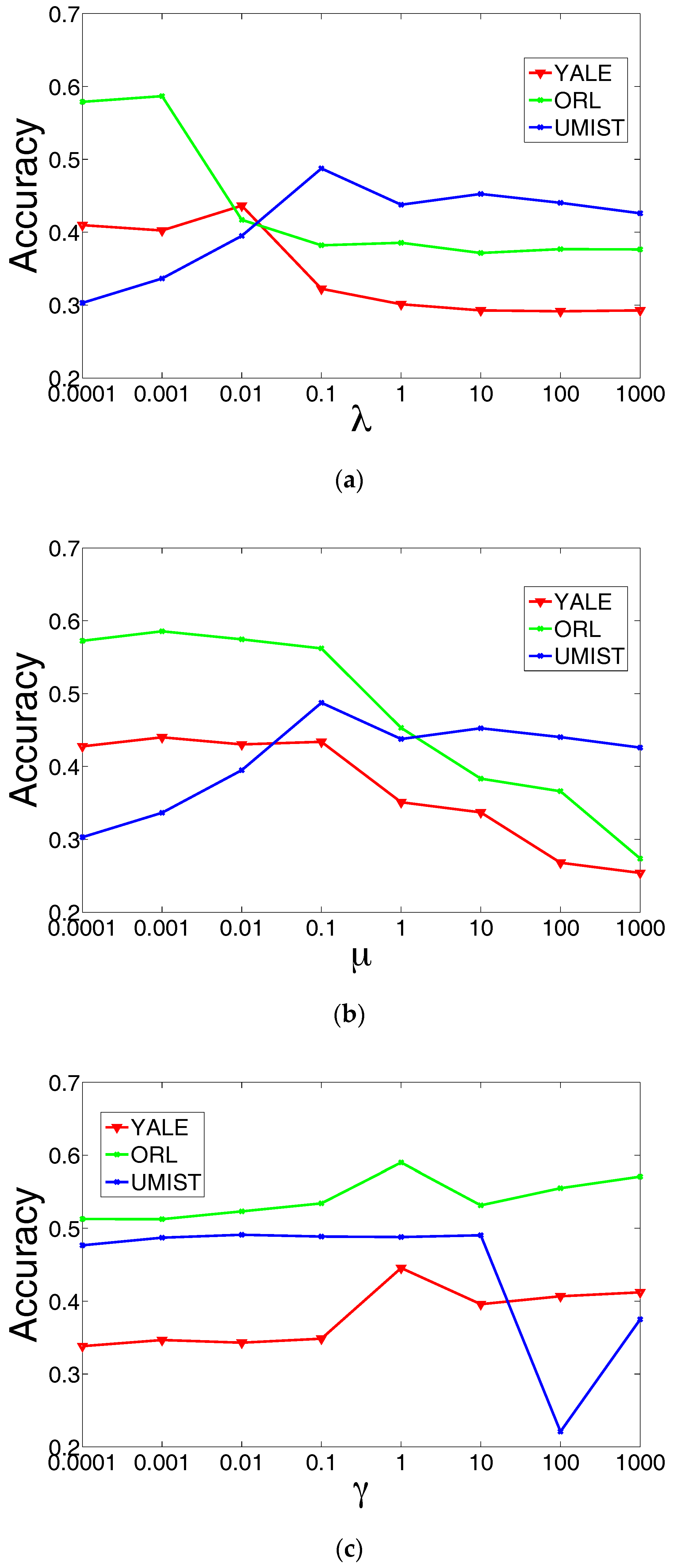
4.5. Parameter Sensitivity

${\ell }_{2,1}$HNMFD has three parameters, $\lambda$, $\mu$ and $\gamma$. We investigated their influence on ${\ell }_{2,1}$HNMFD’s performance by varying one parameter at a time while fixing the other two. For each specific setting, we run ${\ell }_{2,1}$HNMFD 10 times and record the average performance.

We plot the performance of ${\ell }_{2,1}$HNMFD with respect to $\lambda$ in Figure 1a. Parameter $\lambda$ measures the importance of the graph embedding regularization terms of ${\ell }_{2,1}$HNMFD. A too small $\lambda$ may cause graph regularization so weak that the local geometrical information of data cannot be effectively characterize, while too big $\lambda$ may cause a trivial solution. ${\ell }_{2,1}$HNMFD shows superior performance when $\lambda$ equals 0.01, 0.001 and 0.1 for YALE, ORL and UMIST, respectively.

We plot the performance of ${\ell }_{2,1}$HNMFD with respect to $\mu$ in Figure 1b. Parameter $\mu$ controls the orthogonality of the learned representation. When $\mu$ is too small, the orthogonal constraint will be too weak, and ${\ell }_{2,1}$HNMFD may be ill-defined. When $\mu$ is too large, the constraint may dominate the objective function of ${\ell }_{2,1}$HNMFD, and the learned representation will be too sparse, which is also unfaithful to the real-world situation. We can observe that ${\ell }_{2,1}$HNMFD is able to achieve encouraging performance when $\mu$ equals 0.001, 0.001 and 0.1 for YALE, ORL and UMIST respectively.

We plot the performance of ${\ell }_{2,1}$HNMFD with respect to $\gamma$ in Figure 1c. Parameter $\gamma$ controls the degree of sparsity of the encoding matrix. Sparsity constraints that are too weak or too heavy will be bad for the learned representation. We find that ${\ell }_{2,1}$HNMFD consistently outperforms the best baseline methods on the three datasets when $\gamma =1$.

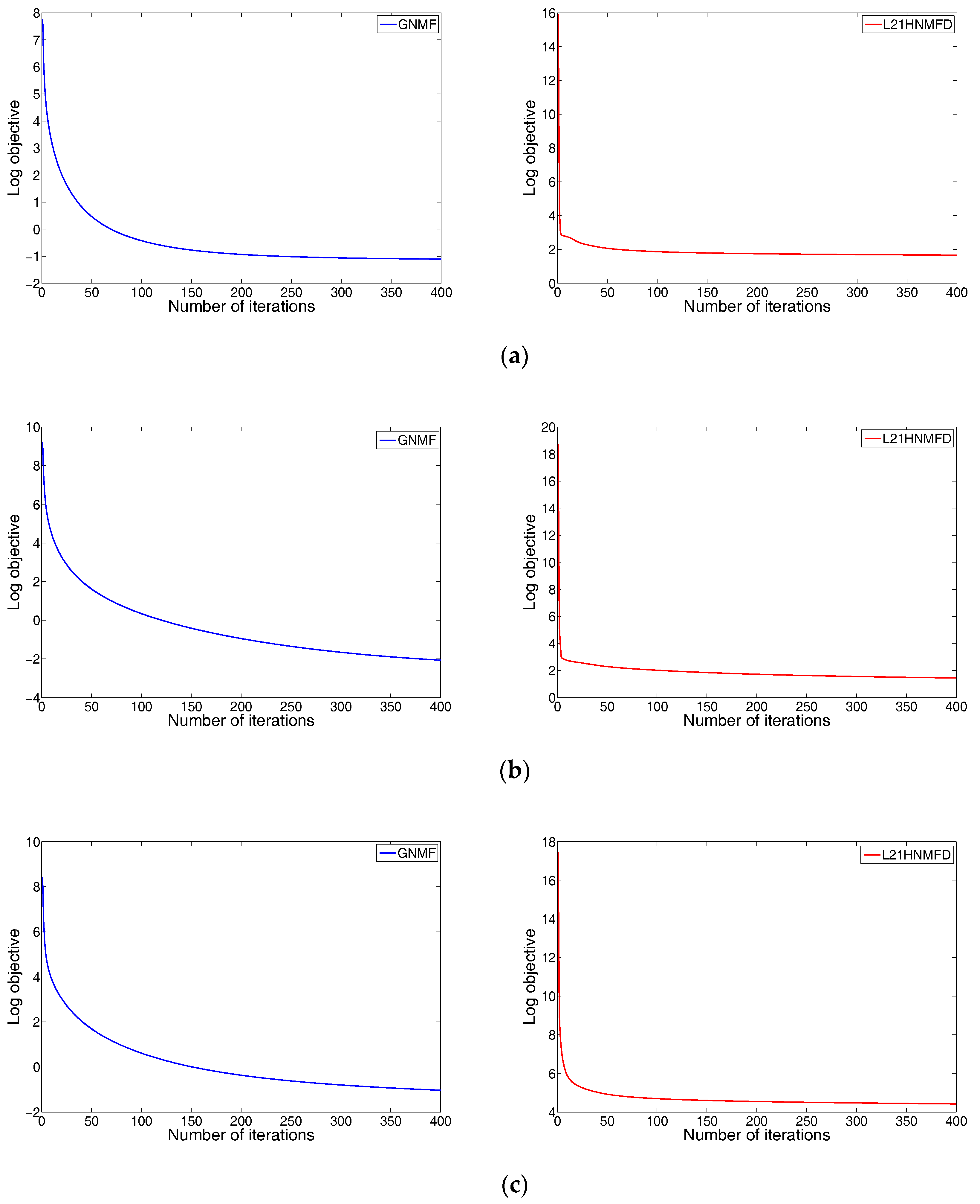
4.6. Convergence Analysis

The updating rules for minimizing the objective function of ${\ell }_{2,1}$HNMFD are essentially iterative. We have provided its convergence proof. Next, we analyze how fast the rules can converge.

We investigate the empirical convergence properties of both GNMF and ${\ell }_{2,1}$HNMFD on three datasets. For each figure, the x-axis denotes the iterative number and the y-axis is the value of objective function with log scale. Figure 2a–c show the objective function value against the number of iterations performed for data set YALE, ORL and UMIST, respectively. We observed that, at the beginning, the objective function values for both GNMF and ${\ell }_{2,1}$HNMFD dropped drastically, and were able to converge very fast, usually within 100 iterations.

5. Conclusions and Future Work

In this paper, we have discussed a novel matrix factorization method, called ${\ell }_{2,1}$ norm and Hessian Regularized Non-negative Matrix Factorization with Discriminability (${\ell }_{2,1}$HNMFD), for data representation. On one hand, ${\ell }_{2,1}$HNMFD uses Hessian regularization to preserve the local manifold structures of data. On the other hand, ${\ell }_{2,1}$HNMFD exploits the ${\ell }_{2,1}$ norm constraint to obtain sparse representation, and uses an approximation orthogonal constraint to characterize the discriminative information of the data. Experimental results on 5 real-world datasets suggest that ${\ell }_{2,1}$HNMFD is able to learn a better part-based representation. This paper only considers single-view cases. In the future, we will consider multi-view cases, and learn a meaningful representation for multi-view data.

References

- Verleysen, M.; François, D. The Curse of Dimensionality in Data Mining and Time Series Prediction. In Proceedings of the Computational Intelligence and Bioinspired Systems, Barcelona, Spain, 8–10 June 2005; pp. 758–770. [Google Scholar]
- Abdi, H.; Williams, L.J. Principal component analysis. Wiley Interdiscip. Rev. Comput. Stat. 2010, 2, 433–459. [Google Scholar] [CrossRef]
- Lee, D.D.; Seung, H.S. Learning the parts of objects by non-negative matrix factorization. Nature 1999, 401, 788–791. [Google Scholar] [PubMed]
- Guillamet, D.; Vitria, J. Classifying faces with nonnegative matrix factorization. In Proceedings of the 5th Catalan Conference for Artificial Intelligence, Castellón, Spain, 24–25 October 2002; pp. 24–31. [Google Scholar]
- Zafeiriou, S.; Petrou, M. Nonlinear non-negative component analysis algorithms. IEEE Trans. Image Process. 2010, 19, 1050–1066. [Google Scholar] [CrossRef] [PubMed]
- Xu, W.; Liu, X.; Gong, Y. Document clustering based on non-negative matrix factorization. In Proceedings of the 26th Annual International ACM SIGIR Conference on Research and Development in Informaion Retrieval, Toronto, ON, Canada, 28 July–1 August 2003; pp. 267–273. [Google Scholar]
- Cai, D.; He, X.; Han, J.; Huang, T.S. Graph regularized nonnegative matrix factorization for data representation. IEEE Trans. Pattern Anal. Mach. Intell. 2011, 33, 1548–1560. [Google Scholar] [PubMed]
- Lu, X.; Wu, H.; Yuan, Y.; Yan, P.; Li, X. Manifold regularized sparse NMF for hyperspectral unmixing. IEEE Trans. Geosci. Remote Sens. 2013, 51, 2815–2826. [Google Scholar] [CrossRef]
- Gu, Q.; Zhou, J. Neighborhood Preserving Nonnegative Matrix Factorization. In Proceedings of the British Machine Vision Conference, London, UK, 7–10 September 2009; pp. 1–10. [Google Scholar]
- Kim, K.I.; Steinke, F.; Hein, M. Semi-supervised regression using Hessian energy with an application to semi-supervised dimensionality reduction. In Proceedings of the Advances in Neural Information Processing Systems, Vancouver, BC, Canada, 7–10 December 2009; pp. 979–987. [Google Scholar]
- Hoyer, P.O. Non-negative matrix factorization with sparseness constraints. J. Mach. Learn. Res. 2004, 5, 1457–1469. [Google Scholar]
- Cai, D.; He, X.; Han, J. Spectral regression: A unified approach for sparse subspace learning. In Proceedings of the Seventh IEEE International Conference on Data Mining (ICDM 2007), Omaha, NE, USA, 28–31 October 2007; pp. 73–82. [Google Scholar]
- Zou, H.; Yuan, M. The F∞-norm support vector machine. Stat. Sin. 2008, 18, 379–398. [Google Scholar]
- Nie, F.; Huang, H.; Cai, X.; Ding, C.H. Efficient and robust feature selection via joint ℓ2,1-norms minimization. In Proceedings of the Advances in Neural Information Processing Systems, Vancouver, BC, Canada, 6–9 December 2010; pp. 1813–1821. [Google Scholar]
- Yang, Y.; Shen, H.T.; Ma, Z.; Huang, Z.; Zhou, X. ℓ2,1-norm regularized discriminative feature selection for unsupervised learning. In Proceedings of the Twenty-Second International Joint Conference on Artificial Intelligence (IJCAI11), Barcelona, Spain, 16–22 July 2011; pp. 1589–1594. [Google Scholar]
- Gu, Q.; Li, Z.; Han, J. Joint feature selection and subspace learning. In Proceedings of the Twenty-Second International Joint Conference on Artificial Intelligence (IJCAI11), Barcelona, Spain, 16–22 July 2011; pp. 1294–1299. [Google Scholar]
- Xu, Z.; Chang, X.; Xu, F.; Zhang, H. L1/2 regularization: A thresholding representation theory and a fast solver. IEEE Trans. Neural Netw. Learn. Syst. 2012, 23, 1013–1027. [Google Scholar] [PubMed]
- Qian, Y.; Jia, S.; Zhou, J.; Robles-Kelly, A. Hyperspectral unmixing via L1/2 sparsity-constrained nonnegative matrix factorization. IEEE Trans. Geosci. Remote Sens. 2011, 49, 4282–4297. [Google Scholar] [CrossRef]
- Wang, W.; Qian, Y. Adaptive L1/2 Sparsity-Constrained NMF With Half-Thresholding Algorithm for Hyperspectral Unmixing. IEEE J. Sel. Top. Appl. Earth Obs. Remote Sens. 2015, 8, 2618–2631. [Google Scholar] [CrossRef]
- Tsinos, C.G.; Rontogiannis, A.A.; Berberidis, K. Distributed Blind Hyperspectral Unmixing via Joint Sparsity and Low-Rank Constrained Non-Negative Matrix Factorization. IEEE Trans. Comput. Imaging 2017, 3, 160–174. [Google Scholar] [CrossRef]
- Li, X.; Cui, G.; Dong, Y. Graph regularized non-negative low-rank matrix factorization for image clustering. IEEE Trans. Cybern. 2016, 1–14. [Google Scholar] [CrossRef] [PubMed]
- Liu, H.; Wu, Z. Non-negative matrix factorization with constraints. In Proceedings of the Twenty-Fourth AAAI Conference on Artificial Intelligence, Atlanta, Georgia, 11–15 July 2010; pp. 506–511. [Google Scholar]
- Li, Z.; Tang, J.; He, X. Robust Structured Nonnegative Matrix Factorization for Image Representation. IEEE Trans. Neural Netw. Learn. Syst. 2017, 1–14. [Google Scholar] [CrossRef] [PubMed]
- Lee, D.D.; Seung, H.S. Algorithms for non-negative matrix factorization. In Proceedings of the Advances in Neural Information Processing Systems 13 (NIPS 2000), Denver, CO, USA, 27 November–2 December 2000; pp. 556–562. [Google Scholar]
- Steinke, F.; Hein, M. Non-parametric regression between manifolds. In Proceedings of the Advances in Neural Information Processing Systems, Vancouver, BC, Canada, 8–10 December 2008; pp. 1561–1568. [Google Scholar]
- Ye, J.; Zhao, Z.; Wu, M. Discriminative k-means for clustering. In Proceedings of the Advances in Neural Information Processing Systems, Vancouver, BC, Canada, 8–10 December 2008; pp. 1649–1656. [Google Scholar]
- Yang, Y.; Xu, D.; Nie, F.; Yan, S.; Zhuang, Y. Image clustering using local discriminant models and global integration. IEEE Trans. Image Process. 2010, 19, 2761–2773. [Google Scholar] [CrossRef] [PubMed]
- Shi, J.; Malik, J. Normalized cuts and image segmentation. IEEE Trans. Pattern Anal. Mach. Intell. 2000, 22, 888–905. [Google Scholar]
Figure 1.
Influence of different parameter settings on the performance of HNMFD in 3 datasets: (a) varying while fixing and ; (b) varying while fixing and ; and (c) varying while fixing and .
Figure 2.
Convergence curve of GNMF and HNMFD. (a) YALE, (b) ORL and (c) UMIST.