Analysis of Powertrain Loading Dynamic Characteristics and the Effects on Fatigue Damage


1
School of Transportation Science and Engineering, Beihang University, Beijing 100191, China
2
Beijing Institute of Space Launch Technology, Beijing 100076, China
*
Author to whom correspondence should be addressed.
Appl. Sci. 2017, 7(10), 1027; https://doi.org/10.3390/app7101027
Submission received: 5 September 2017
/
Revised: 27 September 2017
/
Accepted: 28 September 2017
/
Published: 6 October 2017
(This article belongs to the Section Mechanical Engineering)
Abstract
:The objective of this study is to investigate the effects of key factors on the powertrain loading dynamic characteristics and fatigue damage. First, the engine and the transmission output shaft torque of a multi-axle vehicle powertrain system were measured by proving grounds (PG) testing and analyzed with a conclusion that the powertrain loading changes were mainly related to three key factors: the mean engine torque, the harmonic engine torque, and the vibration properties of the system. Subsequently, a dynamic model considering the three factors was built and validated by the test data. Finally, fatigue damage of shaft parts and gear parts were calculated to investigate the influence degrees of the three factors. The results show that, the harmonic engine torque and the vibration properties of the powertrain system have a great influence on the fatigue damage of shaft parts, and the mean engine torque is the main factor causing the fatigue damage of gear parts.
1. Introduction
With the improving of testing and simulation techniques and the rising demands for the vehicle durability and economy, the fatigue damage analysis technique based on loading spectrum is widely used in reliability and lightweight design. Khosrovaneh et al. [1] examined the effects of the material fatigue properties, stress, or strain results in predicting fatigue life and discussed various mean stress corrections and different methods of accelerating fatigue analysis, along with their advantages and disadvantages. Kim et al. [2] analyzed the operation conditions and working load on the transmission input shaft of an agricultural tractor and discussed the severeness to the transmission of the loading spectra obtained from the different operations. Lee et al. [3] represented the relative fatigue damage analysis technique with the loads of the powertrain system obtained from measurement to analyze the revolution counting for the endurance.
Loading spectrum for fatigue damage analysis is mainly obtained from durability test and computer simulation. In the aspect of durability tests, Grubisic [4] described the criteria and the main parameters of loading spectrum used for design and testing and discussed the procedures to determine these spectra and the requirements concerning the reliability. Lee et al. [5] discussed the analytical methodology and fundamental technical information useful in vehicle powertrain durability testing. Wang et al. [6] presented the multi-criteria decision-making technology to estimate the minimum sample size of the load on a wheel loader transmission under multiple operating conditions. Jambhale et al. [7] developed a complete vehicle loading spectrum test and data processing method based on the specific circumstances of the Indian market. Mattetti et al. [8] defined a methodology to reproduce of real customer tractor usage of tractors in accelerated structural tests. Shih et al. [9] detailed the formulation of the method used by ArvinMeritor for developing a vehicle drive train component test bogey to support product design and development.
In general, obtaining loading spectra by testing requires lots of time and cost. How to predict the fatigue loading spectrum accurately and efficiently by simulation has drawn the attention of researchers. At present, the studies on load spectrum simulation can be mainly divided into two methods: one based on virtual prototype and the other based on available data, which are usually typical condition testing loads or the data of similar models from database.
In the case of simulation methods based on virtual prototype, Joseph et al. [10] developed a virtual powertrain model to simulate the powertrain endurance driving cycle, and the correlation between the predictions and test data collected on a vehicle that was driven through the same driving cycle at PG was made. Haq et al. [11] predicted driveline component loading based on a complete PG schedule with a simulation model. Attibele et al. [12] presented a simple driveline model that was capable of simulating the accelerated endurance cycles as they ran on the PG or on the dynamometer. Then, the simulation results were compared with results of several real world drive cycles for the same vehicle category. In the case of the simulation method based on available data, Wang et al. [13] presented a cyclic simulation approach to generate of the non-stationary loading histories of engineering vehicles based on the Markov chain Monte Carlo method. Wang et al. [14] extrapolated the Rainflow matrix based on a multi-criteria decision-making method with which the proper upcrossing of the high and low levels was determined. Lin et al. [15] compared two data reduction methods based on a simulated staircase test data and two extrapolation methods from shorter fatigue lives, and the results of simulated test were statistically evaluated.
A powertrain system has assorted parts that form a complicated chain through various sorts of connections. The powertrain components work in complex conditions with stochastic excitations that include periodic changes of engine torque, vibrations from road and internal assembly, and impacts caused by shifting, braking, starting, accelerating, and decelerating, etc. Consequently, it is important to identify the key factors that affect fatigue damage in study of loading spectrum simulations. Oelmann [16] analyzed the influence of factors such as rated engine torque, rear axle ratio, transmission ratios, type of transmission, and vehicle mass on the loading spectrum of vehicle components and developed a formula with which conversion of load spectrum from one vehicle to another was possible. Ilie et al. [17] compared the effects of four road conditions on the fatigue life of a transmission output shaft, and analyses showed that the condition with most stop–start events resulted in the greatest reduction to fatigue life.
With the analysis of the loading histories measured by PG testing, this paper investigated the factors that affect loading spectra of powertrain components and fatigue damage based on dynamic simulation methods. The paper is organized as follows. Section 2 introduces the PG testing from which the torque on the engine and the transmission output shafts were obtained and analyzed. In Section 3, a powertrain dynamic model is presented, and the simulated results are validated. In Section 4, virtual experiments of three strategies are designed to simulate the powertrain loading spectra, of which the fatigue damage are calculated for shaft parts and gear parts respectively. Finally, conclusions are presented.
2. Collection and Analysis of Test Loading Spectra
2.1. Rotary Telemetry Torque Measurement System
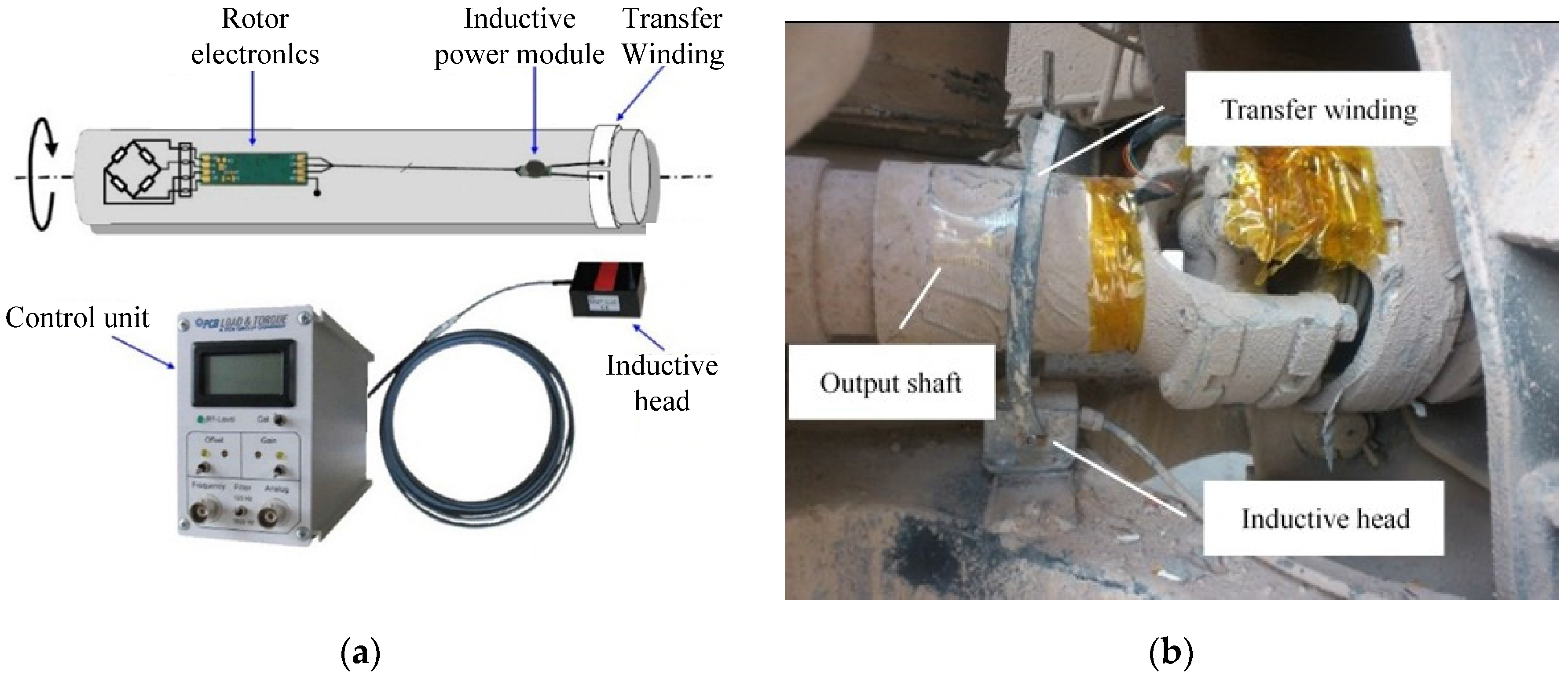
In order to measure the torque on the engine and the transmission output shafts, a rotary telemetry torque measurement system (model 8180) manufactured by PCB Load & Torque, Inc. (Depew, NY, USA) was used. The measurement system consists of a control unit, rotor electronics, an inductive power module, a transfer winding, and an inductive head, as shown in Figure 1a. The rotor electronics, inductive power module, and transfer winding were mounted on the engine and the transmission output shafts, respectively, as shown in Figure 1b. The signals measured by the strain gauge were wirelessly transmitted through the transfer winding to the inductive head and then collected by the control unit. The acquisition software on the computer analyzed the signals and realized the real-time torque on the engine and the transmission output shafts. Additionally, the shaft rotational speeds were recorded by the rotational speed sensors mounted on the flanges of the shafts.
2.2. Data Preprocessing
2.2.1. Data Verification
Transducers are susceptible to external interference such as electrical noise or accidental loads in testing, so the data collected contained unwanted signals like dropouts, spikes, or drifts. Doubtful data were examined to determine whether the signal was invalid or valid, and then the invalid was corrected.
2.2.2. Effective Band Estimation and Sampling Rate
To determine the effective band of the torque signals, a test was implemented with the engine running on the highest speed. The engine output shaft torque was measured with its sampling rate set to 1000 Hz. The power spectrum densities (PSD) of the test data are shown in Figure 2.
The power within the band of and the total power are calculated as follows:
when , it is believed that the effective band is included in [18].
By setting fc to 150 Hz, the checking value of c was 0.995 for the torque on the engine output shaft, and 0.997 for the torque on the transmission output shaft, respectively. So the conclusion was that 0–150 Hz contained the effective band of the signals.
According to reference [17], the sampling rate needs to be at least 22.5 times the signal harmonic frequency, i.e., 3375 Hz, to achieve 1% accuracy in signal peak value.
2.2.3. Data Interpolation and Filtering
Subjected to the performance of the measurement system, the maximum sampling rate was 1000 Hz. In order to improve the accuracy of the measured signals, Hermite interpolation was used with the interpolation frequency set to 4000 Hz.
For the interference and noise signals present in testing and the pseudo-high frequency signals appearing in the interpolation process, the low-pass filter was used before and after interpolating. The upper limit of the effective band, i.e., 150 Hz, was used as the cutoff frequency.
2.3. Analysis of the Test Data
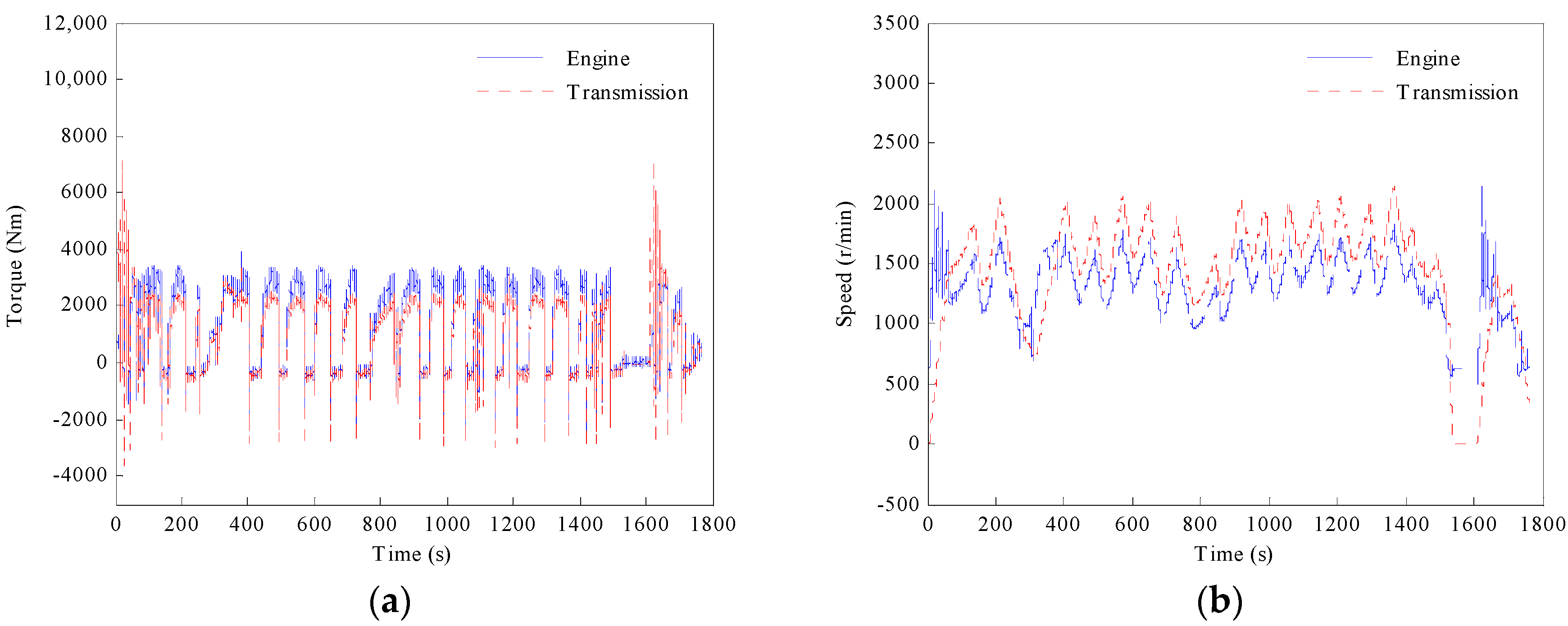
The PG testing included conditions such as gearshift, acceleration, deceleration, turning, and free drive etc. Figure 3 shows a typical testing condition, of which the test time was about 30 min and the maximum speed was 69 km/h. The torque and the rotational speeds of the engine and the transmission output shafts are shown in Figure 3a,b, respectively.
2.3.1. Time Domain Analysis
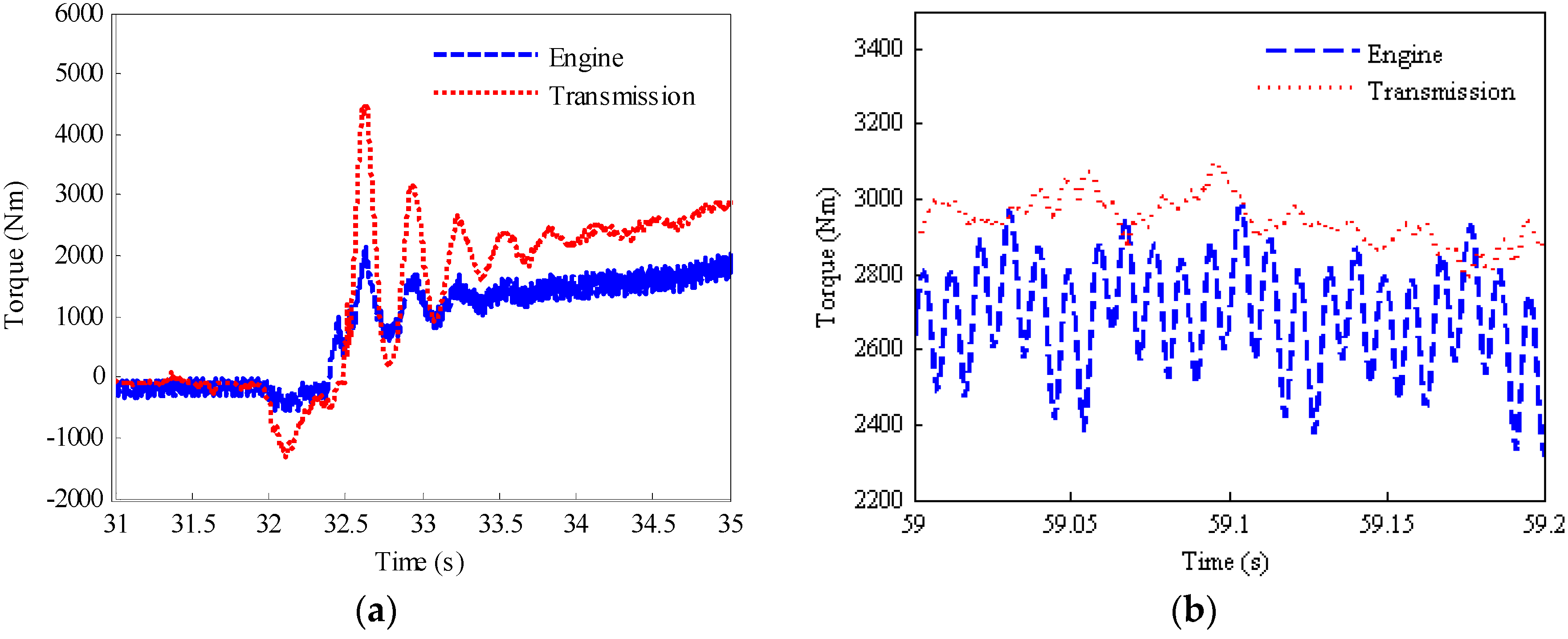
Figure 4 shows the torque fluctuation during shifting and accelerating. It can be seen that there is a torsional oscillation on the engine and transmission output shafts, and the amplitude of the transmission output shaft torque is larger. This phenomenon indicates that there are spring-damper components in the powertrain system. Alone with the impact load generated by clutch in shifting process, the oscillation occurred.
Figure 4b shows a partial enlarged view of the engine and the transmission output shaft torque in acceleration process. It can be seen that the engine torque has a higher frequency as well as a larger amplitude. The transmission output shaft torque is relatively gentle.
2.3.2. Frequency Domain Analysis
The PSD analysis is shown in Figure 5. The result shows that the energy is mainly distributed in three bands: 0–15 Hz (Area 1), 15–30 Hz (Area 2), and 80–125 Hz (Area 3). In Area 1, 0–1 Hz is mainly the mean engine torque, and 1–15 Hz is related to the vibration characteristics of the powertrain. According to the engine rotational speed, analysis indicates that bands of 15–30 Hz and 80–125 Hz are the frequencies of the 1st and the 4th harmonic the engine torque, respectively. From Figure 5, it can be seen that the 1st harmonic has impacts on both the engine and the transmission output shaft torque. However, the 4th harmonic impacted the engine output shaft torque more than the transmission.
2.4. Summary
According to the analysis above, the conclusion is that the powertrain loading is mainly related to the mean engine torque, the harmonic engine torque and the powertrain system vibration properties. Analysis based on dynamic method will be presented to validate this conclusion in the next chapter.
3. Dynamic Analysis of Powertrain System
3.1. System Dynamic Model
3.1.1. Description of the Powertrain System
The powertrain schematic diagram of the 5-axis vehicle is shown in Figure 6. Power of the engine (ENG) is sent through the torque converter (TC, including the pump and the turbine), the clutch (CLU) and the transmission (TRS), assigned to the interaxle differential (IND) by the transfer case (TRC), and then transmitted to the main reducer (MR) and the differential (DIF), eventually delivered to the wheels via the wheel reducer (WR). In this system, an elastic coupling is mounted between the engine and the torque converter, and a torsional damper is mounted between the torque converter and the clutch as well.
3.1.2. System Dynamic Equation
Without regard to the frictions and mechanical losses, the system dynamic equation is
where J is the inertia matrix, C is the damping matrix, K is the stiffness matrix, , , and are the angular displacement, the angular velocity, and the angular acceleration vector of the system, respectively, and T is the torque vector.
When the clutch is in separation, sliding, or engagement status, the system dynamic equations have different forms of expression. As a result, the following two sections were discussed in three cases.
(1) Clutch sliding status
The system is simplified to a model that consists of five rotor inertias and three spring-dampers in clutch sliding state, as shown in Figure 7. The rotor inertia J1 includes the inertias of the engine crankshaft, the flywheel, and the active part of the coupling. The rotor inertia J2 includes the inertia of the coupling passive part, the engine output shaft, and the impeller of the torque converter. The rotor inertia J3 includes the inertia of the turbine of the torque converter, the clutch, the transmission, the transfer case, the bridge gear boxes, the main reducers, the differentials, the wheel reducers, the wheels, and the shafts among them. The rotor inertia J4 is the equivalent inertia of the vehicle. K1, C1, K2, C2, and K3, C3 are the equivalent stiffness and damping of the elastic coupling, the torsional damper, and the tires, respectively. The stiffness and damping of drive shafts are ignored. Te and TR are the engine torque and the equivalent resistant torque, respectively.
The equivalent moment of inertia, stiffness, and damping of the transmission components are calculated as Equation (3),
where , , and are the equivalent moment of inertia, stiffness, and damping, respectively. , , and are the initial moment of inertia, stiffness, and damping, respectively. , , and are the transmission ratios from the engine to the interests.
According to the simplifying work above, we can give the matrixes and vectors in the Equation (2) as follows: the stiffness matrix is ; the damping matrix is ; the inertia matrix is ; the angular displacement vector is ; and the torque vector is . The torque of the clutch in sliding status is calculated by Equation (4),
where is the angular velocity of the active part of the clutch, is the angular velocity of the passive part of the clutch, z is the number of friction plates, is the friction coefficient, is the working pressure applied to the friction plate, and is the average friction radius of the friction plate.
(2) Clutch separation and engagement status
When the clutch is separated, the torque transmitted by the clutch is
The others in Equation (2) are the same as in clutch sliding status.
is no longer determined by Equation (4) but unknown in clutch engagement status. Additional restraint condition is giving by Equation (6):
3.1.3. System Input and Response
(1) The engine torque and vehicle loads
During the operation of the engine, the gas pressure in the cylinder changing continuously causes the fluctuation of torque. The engine torque can be expressed as the superposition of the mean torque and the harmonics [19], expressed as follows:
where is the mean engine torque that was obtained by interpolation based on the engine partial load characteristics surface with the given engine speed and throttle opening degree, is the throttle opening degree, is the engine speed, j is the harmonic order, t is the time, and and are the amplitude and phase angle corresponding to the harmonic order, respectively.
With the acceleration resistance have been considered in Equation (2), the vehicle is subjected to the resistance of wind, rolling and slope. The equivalent resistant torque is
where G is the weight of the vehicle, f is the rolling resistance coefficient, is the slope angle, is the air resistance coefficient, A is the windward area, u (km/h) is the speed of the vehicle, is the wheel rolling radius, and is the total transmission ratio of the powertrain system.
(2) System response
The interests in this article are the torque on the engine and the transmission output shafts. According to the system dynamic equations established above, the system response of , and can be calculated. The torque on the engine and the transmission output shafts can be calculated by Equations (9) and (10),
where , , and are the equivalent inertia moment of the turbine, the clutch, and the transmission, respectively.
3.2. Model Validation
3.2.1. Natural Frequency Analysis
Ignoring the system damping, input and load, the system free vibration equation of the clutch engagement status is
Replacing the acceleration amplitude with the displacement amplitude by , Equation (11) can be derived as
According to the equation of , the system natural frequencies in 8 gears were calculated, as shown in Table 1. The system may have resonance on the natural frequencies but whether or not is also influenced by the system excitations and damping. Further discussion will be presented in the ensuing sections.
3.2.2. Frequency Domain Analysis
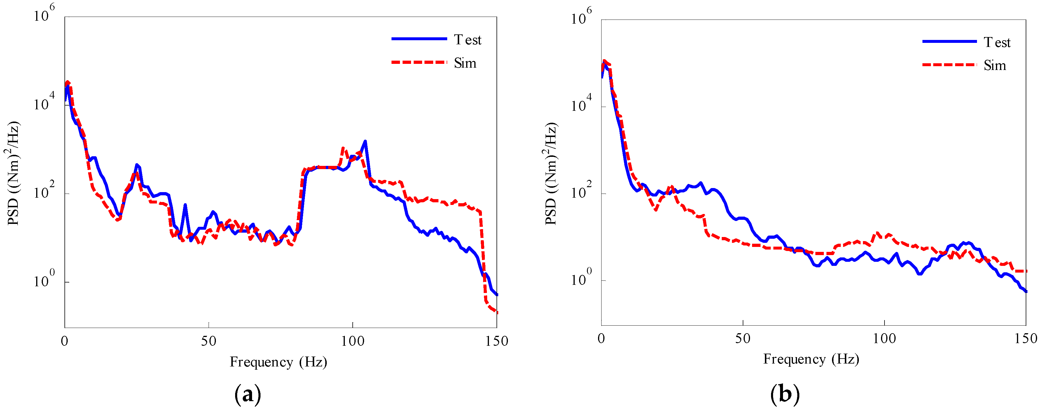
The frequency domain analysis was used to compare the testing and simulation data. Figure 8 shows the PSD of the testing and simulation data. It can be seen that the energies of the engine output shaft torque in the bands of 1st and 4th harmonics are large. In contrast, the transmission output shaft is less affected by the harmonic engine torque.
The 1st order natural frequency signal is mixed with the low-frequency signals that cannot be recognized by PSD analysis. Figure 8a shows that the PSD curve of the engine output shaft torque has peaks at the 2nd and 3rd order natural frequencies but with low energy densities. Figure 8b shows that the PSD curve of the transmission output shaft torque has no obvious peaks at the 2nd and 3rd order natural frequency.
With the analysis above it can be seen that the simulation results of the theoretical model are in good agreement with the experimental data.
3.2.3. Time Domain Analysis
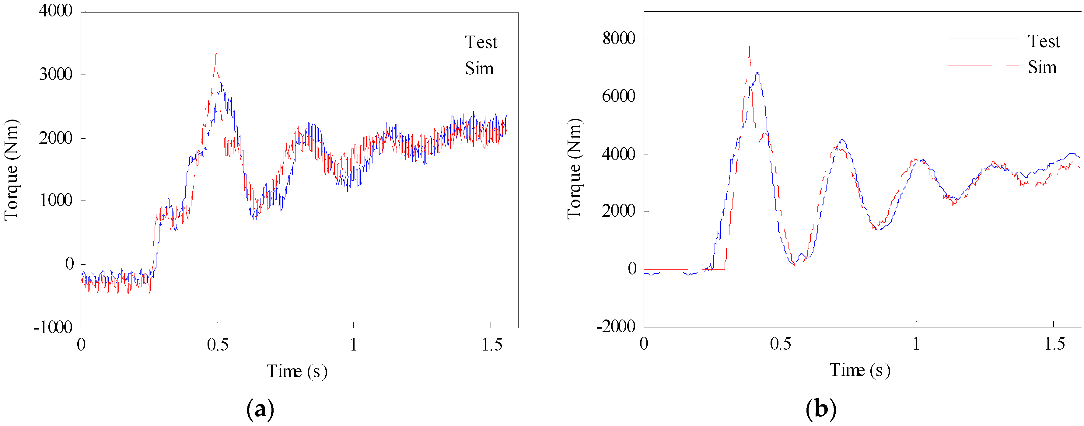
The response in shifting process can reflect the dynamic characteristics of the system. As shown in Figure 9, the comparison of the simulation results and the test data in slipping process and acceleration process after clutch engaged are presented. In the slipping process, the torque of the clutch increases along with the clutch pressure. When the speed difference between the active and the passive parts of the clutch is less than a threshold value, the clutch is engaged. The torque of clutch in the slipping process is large enough that an oscillation, of which the angular frequency corresponds to the 1st order natural frequency of the system, occurs. The amplitude of the oscillation exceeds the maximum torque that the engine can provide.
In the shifting process, both the speed difference between the active and the passive part of the clutch and the pressure applied on the friction plate affect the system dynamic response in shifting process. Consequently it is difficult to simulate the shifting process exactly. The shifting time and the pressure on the friction plate should be checked carefully to make a good agreement between the experimental observations and simulation.
3.3. Summary
According to the analysis above, conclusions can be drawn that the system design avoids the resonance at the 2nd or 3rd order natural frequency, but resonance occurs at the 1st order natural frequency as the impact load in shifting process. The resonance has a large influence on both the engine and transmission output shaft torque. Table 1 shows that the 1st order natural frequency is mainly determined by the low stiffness of the tires.
In addition, the torsional damper dilutes the influence of the harmonic engine torque on the transmission output shaft torque. Nevertheless the elastic coupling doesn’t work well in reducing the vibration of the engine torque so that there are much power of the 1st and the 4th harmonic the engine torque transferred to the engine output shaft as shown in Figure 8a.
4. Fatigue Damage Analysis
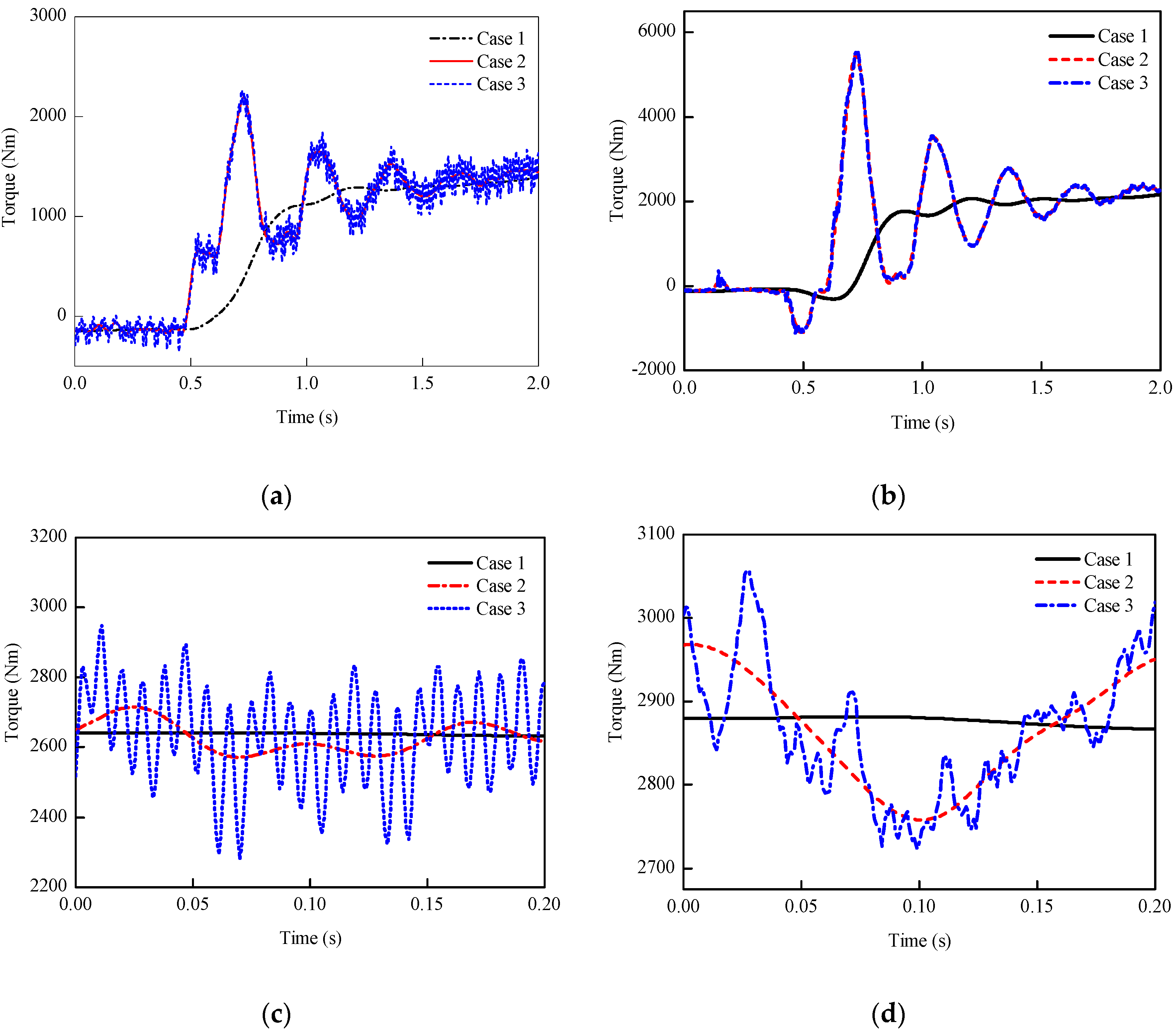
The above research has proved that the powertrain loading profiles are mainly related to the mean and harmonic engine torque, the harmonic engine torque, and the vibration properties of the powertrain system. In order to investigate the influences of the three factors on fatigue damage of the powertrain system components, three strategies were used to simulate the loading histories of PG testing:
- Case 1: with the mean engine torque taking into account, the powertrain system was considered as rigid.
- Case 2: with the mean engine torque taking into account, the spring-damper components in the powertrain system were considered.
- Case 3: both the mean and harmonic engine torque was took into account, and the spring-damper components in the powertrain system was considered.
The simulated results of the three cases are shown in Figure 10. Figure 10a,b show the simulated torque on the engine and the transmission output shafts in shifting process, respectively. Figure 10c,d show a partial enlarged view of the simulated data in acceleration process.
Table 2 shows the statistical results of the three simulation strategies.
The simulation results of the three strategies will be compared by evaluating component fatigue damage with a pseudo-S-N curve, which is applicable in two conditions: one is that the real S-N curve of the material or the component is unknown, and the other is that the calculated fatigue damage is zero when the interests are infinite-life designed. If the pseudo-S-N curve has the same slope as the real one, the calculated pseudo-damage value can evaluate the intensity of the loading on the components concerned relatively [20]. In this paper, the estimated pseudo-S-N curve is set as slope factor k = 5.23, referring to the recommended method in reference [21].
4.1. Rainflow Method
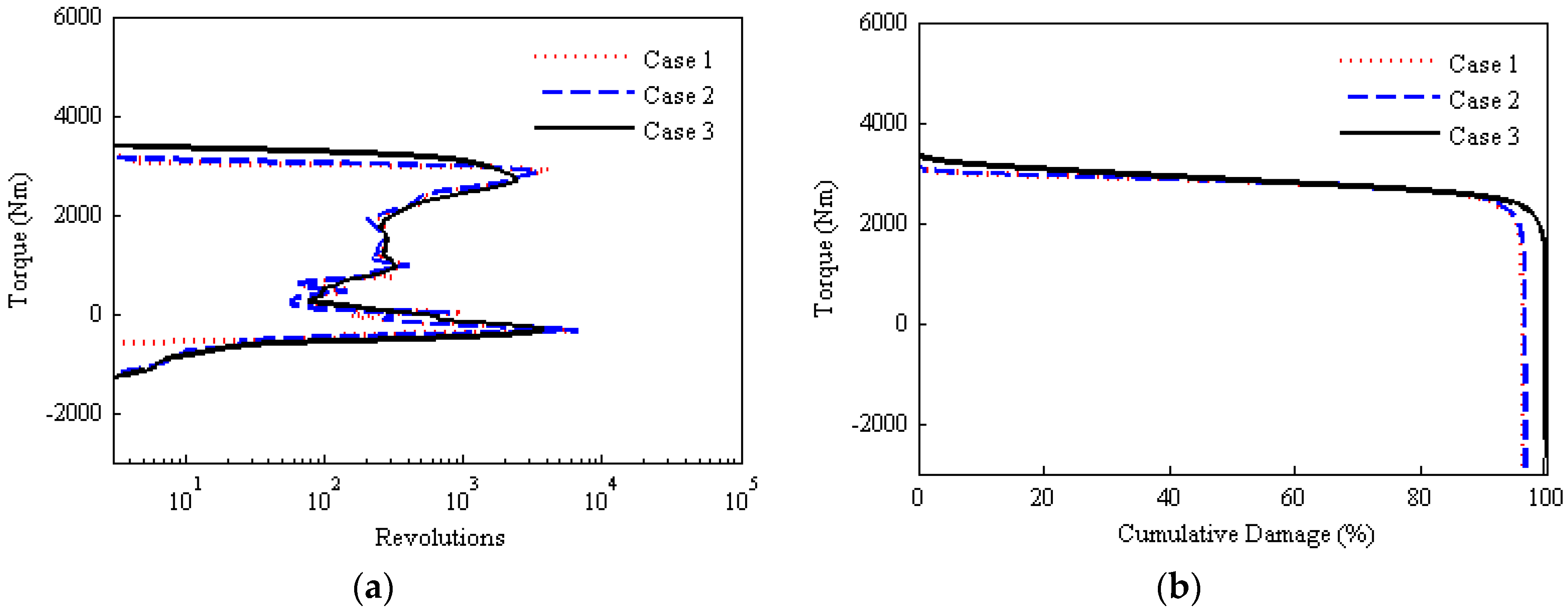
The fatigue damage of shaft parts was calculated by the rainflow method, and the effect of mean stress was corrected by Goodman method. Figure 11 shows the cumulative cycles and cumulative damage of the engine output shaft loading spectrum. The total damage of the third simulation strategy is set as 100%. It can be seen that when the mean engine torque is considered only (in case 1), the cumulative damage is 2.4% and enhances to 8.5% when the impact of elastic damping components in the powertrain system is taken into account.
Furthermore, in Case 3, the loading cycles whose amplitudes are less than 1000 Nm, with 97% of the total cycles, cause about 80% of the total damage. It is easy to recognize that these cycles are produced by the harmonic engine torque. The curves of Case 1 and Case 2 show that the maximum amplitude of the toque reduced when the harmonic torque or the elasticity of the system is ignored. So the conclusion is that, for the torque on the engine output shaft, the harmonic engine torque or the elasticity of the system is non-negligible in calculations of fatigue damage of shaft parts.
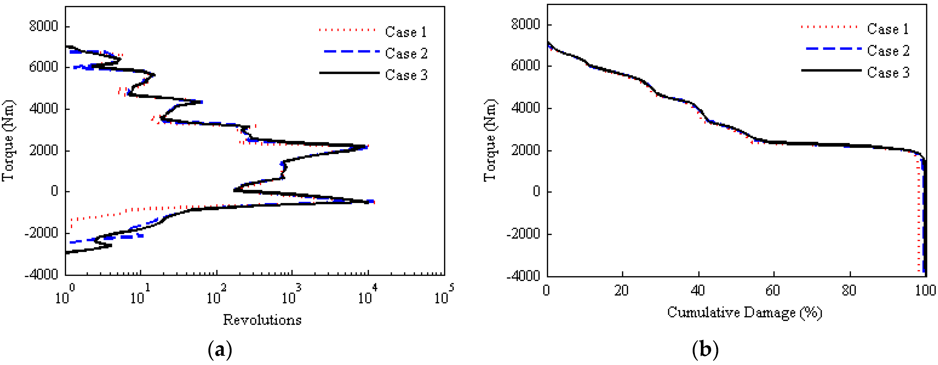
Figure 12 shows the cumulative cycles and cumulative damage of the transmission output shaft torque. Similarly, the total damage of the third simulation strategy is set as 100%. It can be seen that when the mean engine torque is considered only (in case 1), the cumulative damage is 18.8%, and enhances to 79.0% when the impact of spring-damper components in the powertrain system was taken into account. Further analysis shows that the cycles whose amplitudes are more than 8000 Nm, with only about 5% of the total cycles, bring about 79% of the total damage. It can be concluded that for the transmission output shaft toque, the fatigue damage of shaft parts is severely affected by the elasticity of the powertrain system, but little affected by the harmonic engine torque.
4.2. Rotating Moment Histogram (RMH) Method
Different from shaft parts, RMH method was used to calculate the fatigue damage of the gear parts. Figure 13 and Figure 14 show the revolutions and cumulative damage of the engine and the transmission output shaft torque, respectively. The total damage of the third simulation strategy is set as 100%. It can be seen that the cumulative damage is 96.2% when only the mean engine torque is considered (in Case 1), and 96.7% when both the effects of the mean engine torque and the system elasticity are took into account (in Case 2). The RMHs of the three cases have some differences in maximum and minimum torque values, but effects on fatigue damage are little.
Results are similar for the torque on the transmission output shaft. The damage in Case 1 and Case 2 are 98.1% and 99.5%, respectively, of that in Case 3. It can be concluded that the fatigue damage of the transmission output shaft torque for gear parts is mainly caused by the mean engine torque and is little effected by the elasticity of the system and the harmonic engine torque.
4.3. Summary
Analyses results show that the harmonic engine torque and the elasticity of the system has a significant effect on the fatigue damage of shaft parts but little effect on gear parts. In particular, the fatigue damage of the engine output shaft and the transmission output shaft is severely affected by the harmonic engine torque and the elasticity of the powertrain system, respectively.
5. Conclusions
With the studies of the PG testing loading histories, the powertrain dynamic characteristics and the fatigue damage of shaft parts and gear parts, the following conclusions are drawn:
- (1)
- The 5-axle vehicle powertrain loading are mainly decided by three factors: the mean engine torque, the 1st and 4th harmonic engine torque, and the elasticity of the powertrain system.
- (2)
- During the shifting process, the shock torque generated by the clutch produces a greater impact on the engine and the transmission output shafts, and the amplitude of transmission output shaft torque is larger. The 1st harmonic engine torque has effects on both the engine and the transmission output shaft loading. The 4th harmonic engine torque has a great influence on the engine output shaft loading, but little impact on the transmission output shaft loading.
- (3)
- Considering the effects of the stiffness and damping of the elastic coupling, the torsional damper, and the tires, dynamic analysis of the powertrain shows that the 1st order natural frequency coincides with the vibration frequency during shifting process, and the 2nd and 3rd order natural frequencies are not obvious. With the superposition of the mean engine torque, the 1st and 4th harmonic engine torque as system inputs, and the vehicle resistances in driving as system loads, the responses have a good agreement with the experimental data.
- (4)
- For shaft parts, the 4th harmonic engine torque has a great influence on the engine output shaft. The large amount of small loading cycles contribute 80% pseudo-fatigue damage but have little impact on the transmission output shaft. The torque oscillations during shifting process have a greater impact on the fatigue damage of the transmission output shaft torque than the engine output shaft. For gear parts, the mean engine torque constitutes the majority of the pseudo-damage. Regardless of the factors of the harmonic engine torque and the powertrain system, elasticity only results in less than 5% errors.
- (5)
- As the harmonic engine torque and the elastic components have a significant impact on the powertrain loading dynamic characteristics and fatigue damage for shaft parts, further research in optimizing the stiffness and damping of the elastic coupling and torsional damper can be made to reduce the vibration of the system and extend lifetime of components in the future work, while the elasticity of the tire is also non-negligible in analyzing the system characteristics.
Author Contributions
Xuelei Wu and Feng Gao conceived the idea, guide the work and revised the manuscript together; Jinyang designed the work, performed the experiment and the simulation, analyzed the data, make the figures and tables, and wrote the paper; Hongbiao Li contributed to materials and lab facilities, and proof-read the manuscript.
Conflicts of Interest
The authors declare no conflict of interest.
References
- Khosrovaneh, A.; Pattu, R.; Schnaidt, W. Discussion of fatigue analysis techniques in automotive applications. SAE Tech. Pap. 2004. [Google Scholar] [CrossRef]
- Kim, J.H.; Kim, K.U.; Wu, Y.G. Analysis of transmission load of agricultural tractors. J. Terramech. 2000, 37, 113–125. [Google Scholar] [CrossRef]
- Lee, S.H.; Lee, J.H.; Goo, S.H.; Cho, Y.C.; Cho, H.Y. An evaluation of relative damage to the powertrain system in tracked vehicles. Sensors 2009, 9, 1845–1859. [Google Scholar] [CrossRef] [PubMed]
- Grubisic, V. Determination of load spectra for design and testing. Int. J. Veh. Des. 1994, 15, 8–26. [Google Scholar]
- Lee, Y.L.; Haq, S.; Rilly, J.T.; DiDomenico, R.L. Accounting for driver variability in vehicle powertrain durability testing. Int. J. Mater. Prod. Technol. 2002, 17, 434–452. [Google Scholar] [CrossRef]
- Wang, J.; Wang, N.; Wang, Z.; Zhang, Y.; Liu, L. Determination of the minimum sample size for the transmission load of a wheel loader based on multi-criteria decision-making technology. J. Terramech. 2012, 49, 147–160. [Google Scholar] [CrossRef]
- Jambhale, M.S.; Manel, V.A.; Kale, J.G.; Saraf, M.R. Vehicle Response and Real World Driving Pattern for Indian Scenario for Vehicle Development and Optimization Program. SAE Tech. Pap. 2013. [Google Scholar] [CrossRef]
- Mattetti, M.; Molari, G.; Sedoni, E. Methodology for the realisation of accelerated structural tests on tractors. Biosyst. Eng. 2012, 113, 266–271. [Google Scholar] [CrossRef]
- Shih, S.; Kuan, S.; Eschenburg, D. Considerations in the development of durability specifications for vehicle drive train component test. SAE Tech. Pap. 2003. [Google Scholar] [CrossRef]
- Joseph, B.; Attibele, P.; Lee, Y.L.; Haq, S. A PG-based powertrain model to generate component loads for fatigue reliability testing. SAE Tech. Pap. 2003. [Google Scholar] [CrossRef]
- Haq, S.; Joseph, B.; Lee, Y.L.; Taylor, D.; Attibele, P. Vehicle powertrain loading simulation and variability. SAE Tech. Pap. 2004. [Google Scholar] [CrossRef]
- Attibele, P.; Makam, S.; Lee, Y. A Comparison of Real World and Accelerated Powertrain Endurance Cycles for Light-Duty Vehicles. Available online: https://www.nrel.gov/transportation/assets/pdfs/chrysler_paper_posted_with_author_permission.pdf (accessed on 21 April, 2014).
- Wang, J.; Zhang, J.; Liang, Y.; Yang, Y. A cyclic simulation approach for the generation of the non-stationary load histories of engineering vehicles. J. Mech. Sci. Technol. 2012, 26, 1547–1554. [Google Scholar] [CrossRef]
- Wang, J.; Hu, J.; Wang, N.; Yao, M.; Wang, Z. Multi-criteria decision-making method-based approach to determine a proper level for extrapolation of Rainflow matrix. Proc. Inst. Mech. Eng. Part C J. Mech. Eng. Sci. 2012, 226, 1148–1161. [Google Scholar] [CrossRef]
- Lin, S.K.; Lee, Y.L.; Lu, M.W. Evaluation of the staircase and the accelerated test methods for fatigue limit distributions. Int. J. Fatigue 2001, 23, 75–83. [Google Scholar] [CrossRef]
- Oelmann, B. Determination of load spectra for durability approval of car drive lines. Fatigue Fract. Eng. Mater. 2002, 25, 1121–1125. [Google Scholar] [CrossRef]
- Ilie, S.; Ninic, D.; Stark, H.L.; Tordon, M.; Katupitiya, J. Effect of road conditions on the fatigue life of an automatic transmission output shaft. Proc. Inst. Mech. Eng. Part D J. Automob. Eng. 2005, 219, 337–344. [Google Scholar] [CrossRef]
- Zhu, M.W.; Li, Y.X.; Bu, X.Z. Processing and Analysis of Testing Signals, 1st ed.; Beihang University Press: Beijing, China, 2008; p. 86. ISBN 7-81077-923-0. [Google Scholar]
- Walker, P.D.; Zhang, N. Modelling of dual clutch transmission equipped powertrains for shift transient simulations. Mech. Mach. Theory 2013, 60, 47–59. [Google Scholar] [CrossRef]
- Kim, C.-J. Accelerated Sine-on-Random Vibration Test method of ground vehicle components over conventional single mode excitation. Appl. Sci. 2017, 7, 805. [Google Scholar] [CrossRef]
- Lee, Y.L.; Pan, J.; Hathaway, R.; Barkey, M. Fatigue Testing and Analysis, 1st ed.; Elsevier Inc.: Burlington, NJ, USA, 2005; pp. 127–140. [Google Scholar]
Figure 1.
Rotary telemetry torque measurement system: (a) system configuration; (b) installation of the system.
Figure 1.
Rotary telemetry torque measurement system: (a) system configuration; (b) installation of the system.

Figure 2.
Power spectrum densities (PSD) of the highest speed test data.
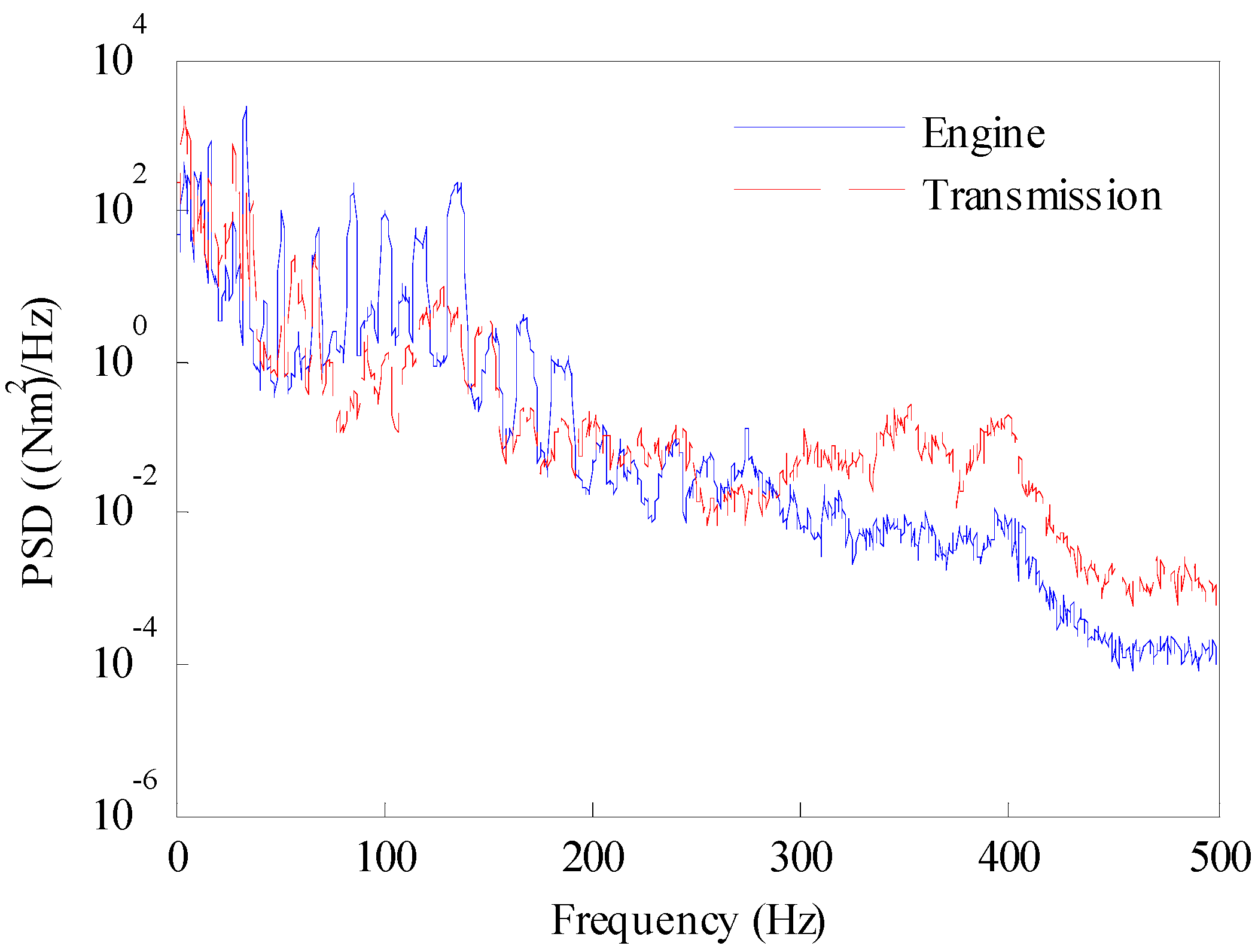
Figure 3.
The proving grounds (PG) test data. (a) Torque signals; (b) rotational speed signals.

Figure 4.
Time domain signals of (a) shifting process and (b) acceleration process (partial enlarged view).
Figure 4.
Time domain signals of (a) shifting process and (b) acceleration process (partial enlarged view).

Figure 5.
PSD analysis of torque on the engine and transmission output shaft.
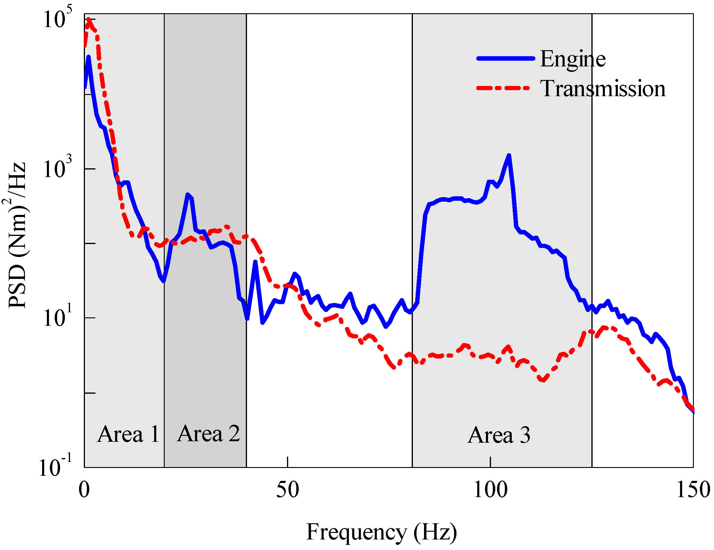
Figure 6.
5-axle vehicle’s powertrain system schematic diagram.
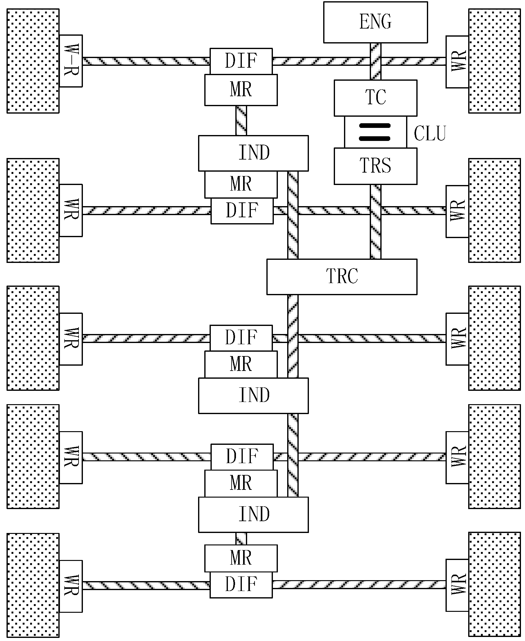
Figure 7.
The simplified model of the powertrain system.
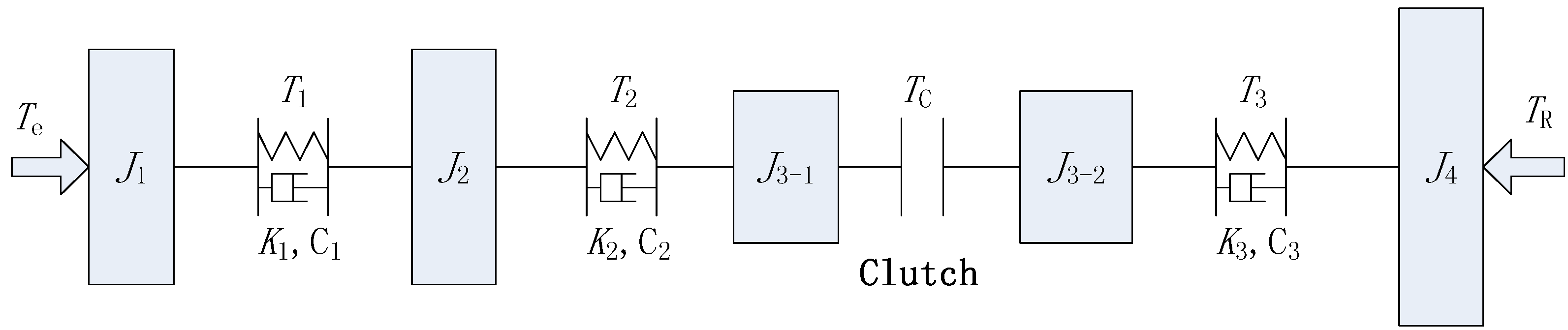
Figure 8.
PSD analysis (a) of the engine output torque and (b) the transmission output torque.

Figure 9.
Comparison of simulation and test data in shifting process. (a) Torque on the engine output shaft; (b) torque on the transmission output shaft.
Figure 9.
Comparison of simulation and test data in shifting process. (a) Torque on the engine output shaft; (b) torque on the transmission output shaft.

Figure 10.
Results of the three simulation strategies: (a) engine torque in shifting process; (b) transmission torque in shifting process; (c) partial enlarged view of engine torque; (d) partial enlarged view of transmission torque.
Figure 10.
Results of the three simulation strategies: (a) engine torque in shifting process; (b) transmission torque in shifting process; (c) partial enlarged view of engine torque; (d) partial enlarged view of transmission torque.

Figure 11.
Fatigue damage analysis of the engine output shaft torque for shaft parts: (a) torque vs. cumulative cycle count (%); (b) torque vs. cumulative damage (%).
Figure 11.
Fatigue damage analysis of the engine output shaft torque for shaft parts: (a) torque vs. cumulative cycle count (%); (b) torque vs. cumulative damage (%).
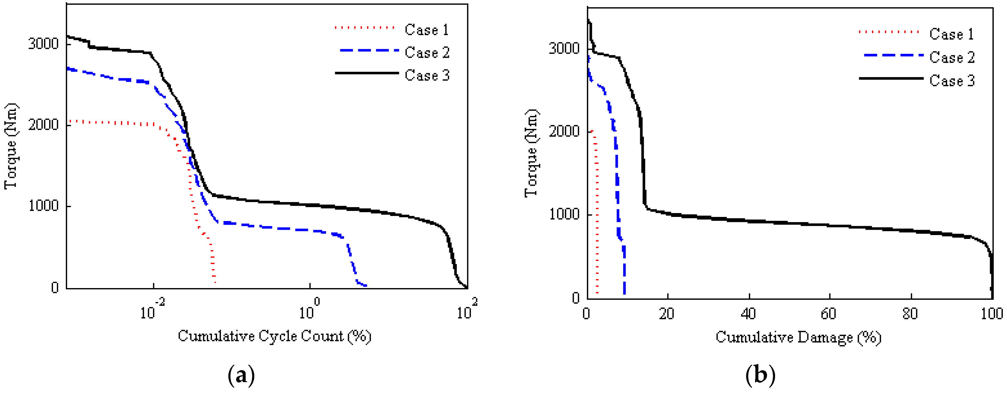
Figure 12.
Fatigue damage analysis of the transmission output shaft torque for shaft parts: (a) torque vs. cumulative cycle count (%); (b) torque vs. cumulative damage (%).
Figure 12.
Fatigue damage analysis of the transmission output shaft torque for shaft parts: (a) torque vs. cumulative cycle count (%); (b) torque vs. cumulative damage (%).
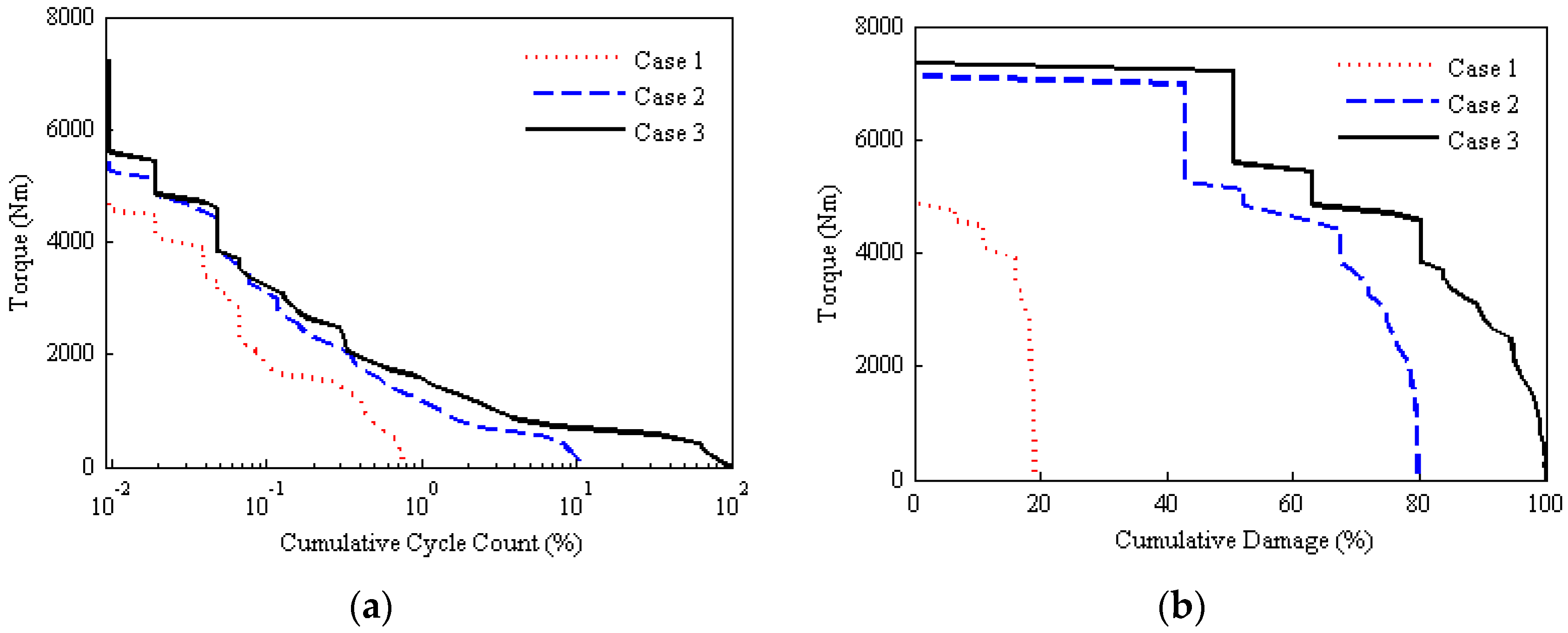
Figure 13.
Rotating moment histogram (RMH) analysis of the engine output shaft toque: (a) torque vs. revolutions (b) torque vs. cumulative damage (%).
Figure 13.
Rotating moment histogram (RMH) analysis of the engine output shaft toque: (a) torque vs. revolutions (b) torque vs. cumulative damage (%).

Figure 14.
RMH analysis of the transmission output shaft toque: (a) torque vs. revolutions; (b) torque vs. cumulative damage (%).
Figure 14.
RMH analysis of the transmission output shaft toque: (a) torque vs. revolutions; (b) torque vs. cumulative damage (%).


Table 1.
The natural frequency analysis of the powertrain system.
| Gear | Moment of Inertia (kg m2) | Stiffness (Nm/rad) | Natural Frequency (Hz) | |||||||
|---|---|---|---|---|---|---|---|---|---|---|
| J1 | J2 | J3 | J4 | K1 | K2 | K3 | 1 | 2 | 3 | |
| 1 | 14.608 | 1.309 | 2.6 | 5.0 | 23,000 | 50,000 | 479 | 2.4 | 12.7 | 42.3 |
| 2 | 2.7 | 11.3 | 1083 | 2.7 | 12.8 | 42.1 | ||||
| 3 | 2.9 | 24.2 | 2300 | 3.0 | 13.0 | 41.8 | ||||
| 4 | 3.4 | 49.2 | 4682 | 3.5 | 13.4 | 41.4 | ||||
| 5 | 4.2 | 104.7 | 9964 | 4.0 | 14.2 | 40.7 | ||||
| 6 | 6.4 | 236.7 | 22,510 | 4.5 | 15.2 | 39.8 | ||||
| 7 | 10.7 | 502.6 | 47,810 | 4.9 | 16.0 | 39.0 | ||||
| 8 | 19.2 | 1024.2 | 97,420 | 5.0 | 16.6 | 38.5 | ||||
Table 2.
Statistical results of the three simulation strategies (unit: Nm).
| Channel | Minimum | Maximum | Mean | MAX RANGE | Std Deviation | RMS | |
|---|---|---|---|---|---|---|---|
| Engine | Case 1 | −596.518 | 3201.51 | 1344.351 | 3798.028 | 1371.193 | 1920.273 |
| Case 2 | −1848.1 | 3581.597 | 1344.412 | 5429.697 | 1376.596 | 1924.177 | |
| Case 3 | −2351.01 | 3947.91 | 1344.412 | 6298.921 | 1382.514 | 1928.416 | |
| Transmission | Case 1 | −1697.73 | 6748.207 | 1064.202 | 8445.938 | 1264.079 | 1652.398 |
| Case 2 | −3540.17 | 9208.032 | 1064.249 | 12748.2 | 1275.829 | 1661.435 | |
| Case 3 | −3666.31 | 9522.35 | 1064.249 | 13188.66 | 1276.794 | 1662.175 | |
© 2017 by the authors. Licensee MDPI, Basel, Switzerland. This article is an open access article distributed under the terms and conditions of the Creative Commons Attribution (CC BY) license (http://creativecommons.org/licenses/by/4.0/).
Share and Cite
MDPI and ACS Style
Bai, J.; Wu, X.; Gao, F.; Li, H. Analysis of Powertrain Loading Dynamic Characteristics and the Effects on Fatigue Damage. Appl. Sci. 2017, 7, 1027. https://doi.org/10.3390/app7101027
AMA Style
Bai J, Wu X, Gao F, Li H. Analysis of Powertrain Loading Dynamic Characteristics and the Effects on Fatigue Damage. Applied Sciences. 2017; 7(10):1027. https://doi.org/10.3390/app7101027
Chicago/Turabian StyleBai, Jinyang, Xuelei Wu, Feng Gao, and Hongbiao Li. 2017. "Analysis of Powertrain Loading Dynamic Characteristics and the Effects on Fatigue Damage" Applied Sciences 7, no. 10: 1027. https://doi.org/10.3390/app7101027
Note that from the first issue of 2016, this journal uses article numbers instead of page numbers. See further details here.