Parameters Sensitivity Analysis of Position-Based Impedance Control for Bionic Legged Robots’ HDU

1
School of Mechanical Engineering, Yanshan University, Qinhuangdao 066004, China
2
Hebei Provincial Key Laboratory of Heavy Machinery Fluid Power Transmission and Control, Qinhuangdao, China
3
National Engineering Research Center for Local Joint of Advanced Manufacturing Technology and Equipment, Yanshan University, Qinhuangdao 066004, China
*
Author to whom correspondence should be addressed.
Appl. Sci. 2017, 7(10), 1035; https://doi.org/10.3390/app7101035
Submission received: 2 September 2017
/
Revised: 27 September 2017
/
Accepted: 30 September 2017
/
Published: 10 October 2017
(This article belongs to the Special Issue Bio-Inspired Robotics)
Abstract
:For the hydraulic drive unit (HDU) on the joints of bionic legged robots, this paper proposes the position-based impedance control method. Then, the impedance control performance is tested by a HDU performance test platform. Further, the method of first-order sensitivity matrix is proposed to analyze the dynamic sensitivity of four main control parameters under four working conditions. To research the parameter sensitivity quantificationally, two sensitivity indexes are defined, and the sensitivity analysis results are verified by experiments. The results of the experiments show that, when combined with corresponding optimization strategies, the dynamic compliance composition theory and the results from sensitivity analysis can compensate for the control parameters and optimize the control performance in different working conditions.
1. Introduction
Bionic legged robots are better at adapting to unknown and unstructured environments. Their unique advantages, such as overcoming obstacles and executing tasks in the wild, have made them a major focus of research in the robotic domain [1,2,3,4]. For the hydraulic drive robot, the highly integrated valve-controlled cylinder composes the drive component, which is called the hydraulic drive unit (HDU) [5,6]. During the robotic motion process, the robotic feet interact with the ground frequently. This means that the demand for HDU not only includes characteristics of response ability and high control accuracy, but also dynamic compliance. Thus, the impact on the hydraulic system can be obviously reduced, which can protect the mechanical structure and components, and improve the moving stability of the robots.
The selection of control methods directly affects the compliance of the HDU. As a commonly used control method for compliance, the impedance control method has been widely applied to motor-driving legged robots such as the Tekken [7], Scout [8] and MIT cheetah robot [9]. In recent years, as the hydraulic-driven legged robot became the focus of increased research, impedance control was also applied to this kind of robot, as exemplified by robots such as Bigdog [10], HyQ [11], and Scalf-1 [12]. Force-based and position-based impedance control methods are often used for dynamic compliance control. Their basic principle can be expressed as follows. Firstly, the hydraulic control system is taken as the control inner loop, and a dynamic control outer loop is attached to the system. When an external disturbance acts on the system, the input signal of the control inner loop can be changed through the control outer loop. Thus, the system is able to possess the desired dynamic compliance.
In this paper, position-based impedance control is the focus of research. There are many parameters in hydraulic systems, such as structure parameters, working parameters, and control parameters. Considering the uncertainty of the parameter variation, the system cannot reach the ideal performance, which involves the effects of parameter variation on robot’s overall compliance. So, in order to optimize the system more efficiently, it is necessary to know how greatly the parameters, particularly the main control parameters, influence the impedance control performance. The parameters that affect the system more should be compensated and optimized emphatically, while the ones that affect system less can be ignored. Thus, the effect of parameter variation on system dynamic characteristics can be quantificationally analyzed, and the analysis results can be used to optimize the robot’s compliance performance. Sensitivity analysis is used to analyze the effect of parameter variation on system characteristics for both linear and nonlinear systems. By computing methods, sensitivity analysis methods can be classified into the trajectory sensitivity method, output sensitivity method, matrix sensitivity method, comparison sensitivity method, characteristic root sensitivity method, etc. By computing accuracy, sensitivity analysis methods can be classified into ties of first-order sensitivity method, second-order sensitivity method, or high-order sensitivity method. These methods have different characteristics in computing; they differ from each other in aspects such as computing accuracy, computing mode, and computing complexity. These differences give each method unique advantages and application ranges. In recent years, sensitivity analysis methods have been commonly used in many fields, but only a few have been applied to hydraulic systems. Vilenus et al. [13] is the first scholar to apply first-order sensitivity analysis to hydraulic systems. For the position control system of valve-controlled cylinders, the sensitivity of 10 main parameters when they changed 1% in a single working condition is researched. Farasat et al. [14] built a fourth-order linear mathematical model for the position control system of valve-controlled cylinders. In the model, the valve’s pressure-flow nonlinearity is partly linearized. Based on Vilenus’s research, he showed the first-order sensitivity analysis results of an extra seven parameters, and proposed four assessment methods to quantify the sensitivity of state variables when parameters changed by 1%. Kong et al. [15] built a fifth-order linear mathematical model for the position-based control system, and studied the effect on system output when 14 system parameters changed by 1%. Based on the first-order trajectory sensitivity, Kong et al. [16] deduced the method of second-order trajectory sensitivity and analyzed the effect on system output when 14 system parameters changed from 1% to 20%. Moreover, experiments are also conducted to verify the effect.
In the position-based impedance control system, the above achievements adopted first-order and second-order sensitivity analysis methods to study the effect on control characteristics when parameters change. However, the above papers didn’t analyze the impedance control methods on HDU. In addition, the trajectory sensitivity analysis methods they used, particularly the second-order trajectory sensitivity analysis method, are very difficult to compute. To solve the two problems, this paper is organized as follows. First, based on the mathematical model of HDU position control system, the method of position-based impedance control is deduced and tested by experiments. Then, to solve the difficulties in sensitivity computing, matrix sensitivity analysis, an easier method, is adopted to analyze the sensitivity of four main control parameters. Further, to obtain the optimal method, the results from matrix sensitivity analysis are compared with the results from trajectory sensitivity analysis. Moreover, the quantificational analysis results of the four main parameters are shown in this paper. Finally, the sensitivity analysis results are verified by experiments.
2. Introduction of the HDU and Its Performance Test Platform
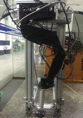
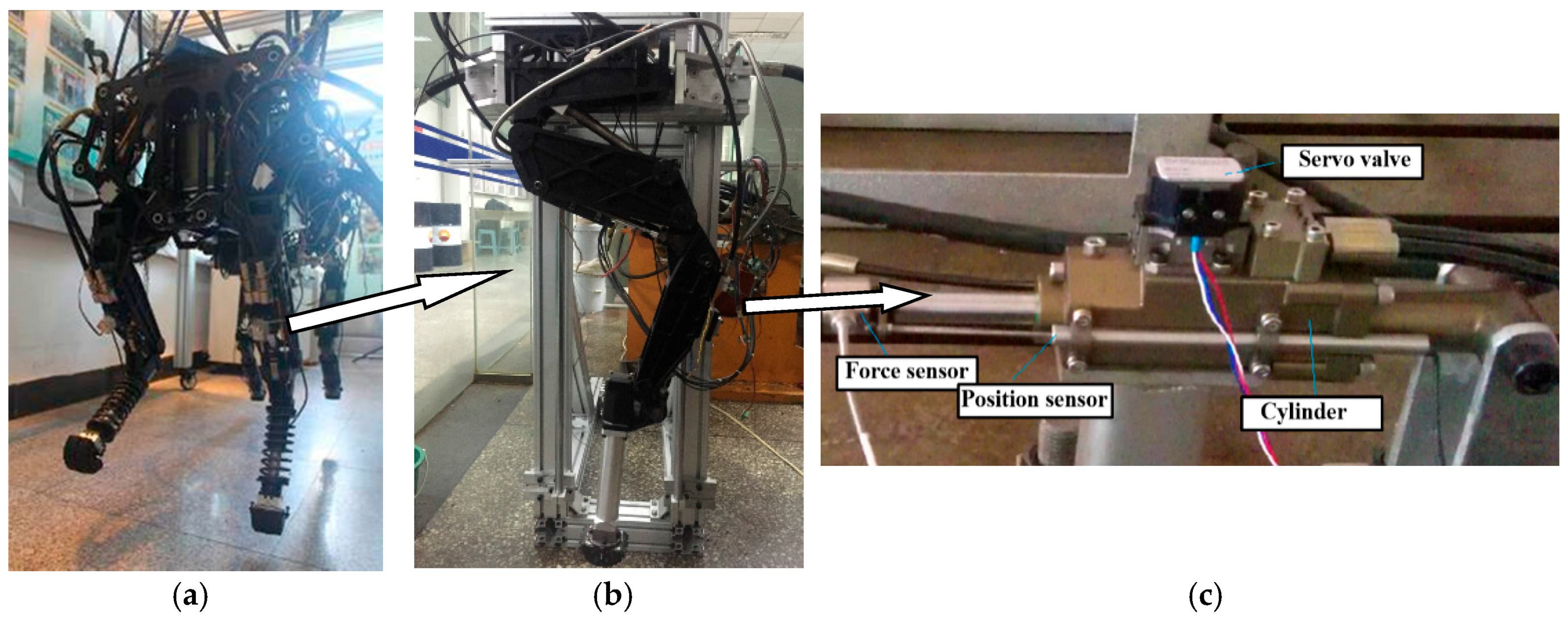
As the driver of the leg joint on bionic legged robots, the HDU is a highly integrated system of servo valve-controlled symmetrical cylinder. The author’s institute participates in the design of the hydraulic quadruped robot. The quadruped robot prototype, single leg, and HDU performance test platform are shown in Figure 1a–c, respectively.
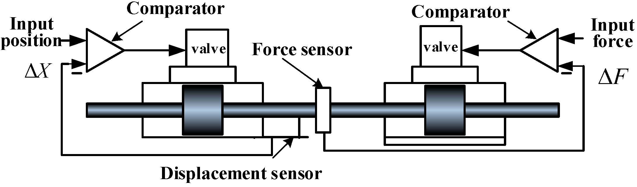
The performance of the HDU directly affects the performance of the whole robot. Thus, a special performance test platform is built to study the methods for HDU. The schematic of the test platform is shown in Figure 2.
The principle of the electro-hydraulic load simulator in Figure 2 is widely used in many fields such as aviation, aerospace, and vessel and construction machining [5]. In Figure 2, the left part is a HDU-adopted position closed-loop control that contains a small servo valve, servo cylinder, position sensor, and force sensor. The right part is another HDU-adopted force closed-loop control that contains the same type of servo valve and servo cylinder. Two parts’ cylinder rods are jointed rigidly by the thread of a force sensor. The HDU performance test platform is showed in Figure 3a. The controller adopted is dSPACE, a semi-physical simulation platform, which is showed in Figure 3b.
3. HDU Position-Based Impedance Control
3.1. Mathematic Model of HDU Position-Based Impedance Control
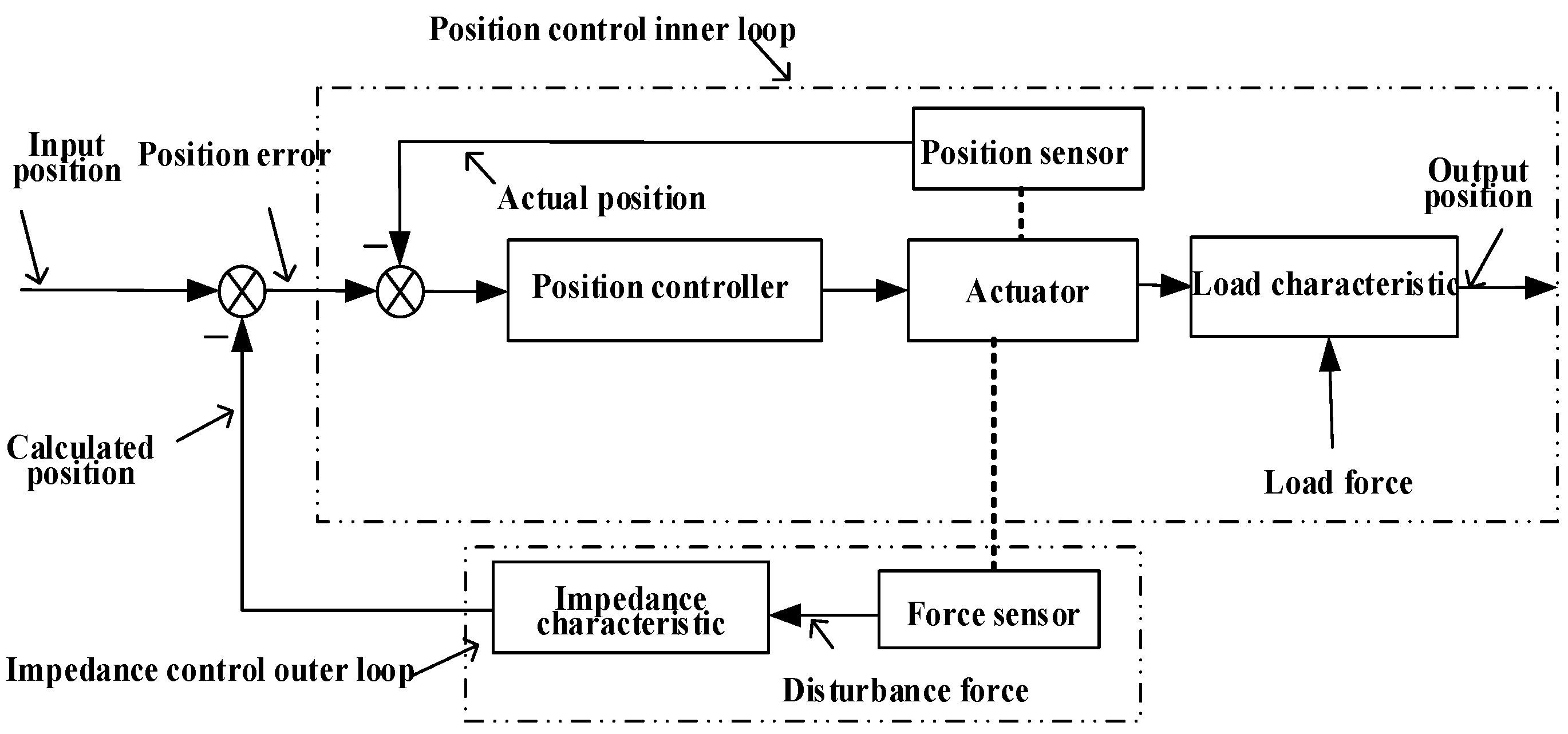
Impedance control is one type of active compliance control. In particular, it refers to an active compliance control that applies the system equivalent to the second-order mass-spring-damping system. By adopting impedance control, a system can be equipped with the dynamic compliance of a second-order mass-spring-damping system when a disturbance force is applied to the system.
The impedance control is composed by an impedance control inner loop and impedance control outer loop. The impedance control inner loop refers to the closed-loop control, which is realized in the inner loop of the hydraulic position closed-loop control system during the impedance control. In the position-based impedance control of this paper, the impedance control inner loop refers to the position closed-loop control. The impedance control outer loop refers to the open-loop control where the external disturbance signal is transferred to the input signal of impedance control inner loop during the impedance control.
3.1.1. Principles of Impedance Control
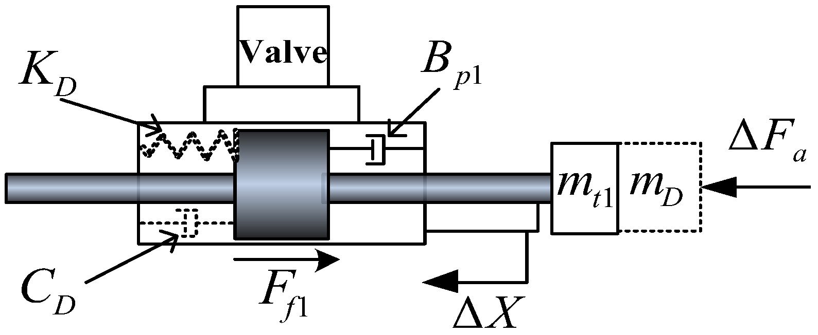
The inner loop of the position-based impedance control is a closed-loop control. When the inner loop is affected by a disturbance force, the impedance control outer loop should be added to the system to equip the system with impedance control characteristics. The function of this outer loop is to transform the disturbance force into position error. Then, the desired stiffness can be obtained, which causes an elastic force. In the same way, desired damping and desired mass are obtained, which can cause viscous force and inertia force, respectively. The HDU force schematics with impedance control outer loop are shown respectively in Figure 4 and Figure 5.
During the robot’s walking process, the load, such as grounds and steps, provides the disturbance force to the HDU, because the force sensor is mounted on the piston end of the HDU. In this paper, the force control system of the simulated load provides the disturbance force to the performance test platform.
As it is shown in Figure 4, the load is pressed to position , refers to damping coefficient at load, refers to equivalent mass at load, and refers to friction at load. The force acting on the piston, which is provided by the sensor, is the disturbance force of the HDU position control system, and is defined as . Further, the force acting on the load, which is provided by the sensor, is defined as . The force balance relation in Figure 4 can be expressed as follows:
Third, the force schematic of the HDU is showed in Figure 5.
Where refers to the viscous damping coefficient, refers to the equivalent mass at piston, and refers to friction in the cylinder. The position error can be expressed as follows:
Based on the theoretical analysis above, the schematic of the position-based impedance control is shown in Figure 6.
As can be seen in Figure 6, when the disturbance force tested by the force sensor acts on the HDU, the impedance control outer loop generates a corresponding calculated position that disturbs the input position. Then, the new input to the position control system is formed. Thus, the final input signal enters the position control inner loop, and a new output position is formed to equip the system with impedance characteristics.
3.1.2. The Block Diagram and State Space Presentation of Impedance Control System
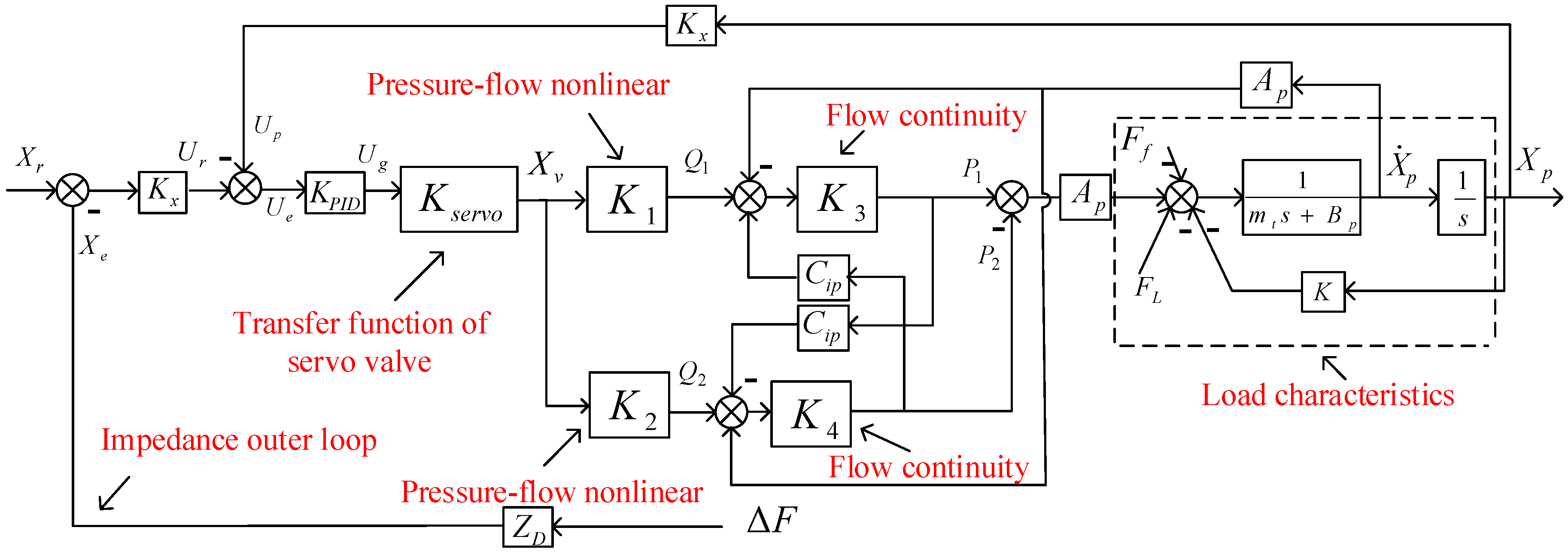
The block diagram of HDU position-based impedance control is shown in Figure 7, where the detailed deduction and performance analysis of the inner loop is presented in previous research [5,15].
In Figure 7, is conversion mass (including the piston, the displacement sensor, the force sensor, the connecting pipe, and the oil in the servo cylinder),
is input position, is position sensor gain, is proportion-integration-differentiation (PID) controller gain including proportional gain , integral gain and differential gain , is load stiffness, is load damping, is load force, is servo valve spool displacement, is servo cylinder piston displacement, is volume of input oil pipe, is volume of output oil pipe, is friction, is input voltage, is controller output voltage, is inlet oil flow, and is outlet oil flow.
Denote,
where is the transfer function of the servo valve, is the natural frequency of the servo valve, is the damping ratio of the servo valve, and is the servo valve gain.
where, and express the transfer function of nonlinear pressure flow, ( is defined as conversion coefficient in this paper), is the orifice flow coefficient of the spool valve, is the area gradient of the spool valve, is the density of hydraulic oil, is the system supply’s oil pressure, is the left cavity pressure of the servo cylinder, is the right cavity pressure of the servo cylinder, and is the system return oil pressure.
where, and express the transfer function of flow continuity, represents the total piston stroke of the servo cylinder, is the initial piston position of the servo cylinder, is the internal leakage coefficient of the servo cylinder, is the external leakage coefficient of the servo cylinder, is the effective piston area of the servo cylinder, and is the effective bulk modulus.
The state variables in Figure 7 are expressed as follows:
where the input variables are expressed as follows:
,
Disturbance variables are expressed as follows:
The state space of the system can be expressed as follows:
The physical meanings and initial values of the parameters in the control system block diagram are shown in Table 1.
3.2. Experiment of Position-Based Impedance Control
As a typical signal, the sinusoidal response is able to evaluate the impedance control performance under the input of different frequencies and amplitudes. In this paper, a sinusoidal signal is adopted to analyze the system performance and the sensitivity of the main parameters. To study their variation patterns in different conditions, four working conditions are tested in this paper. The details of the working conditions are shown in Table 2.
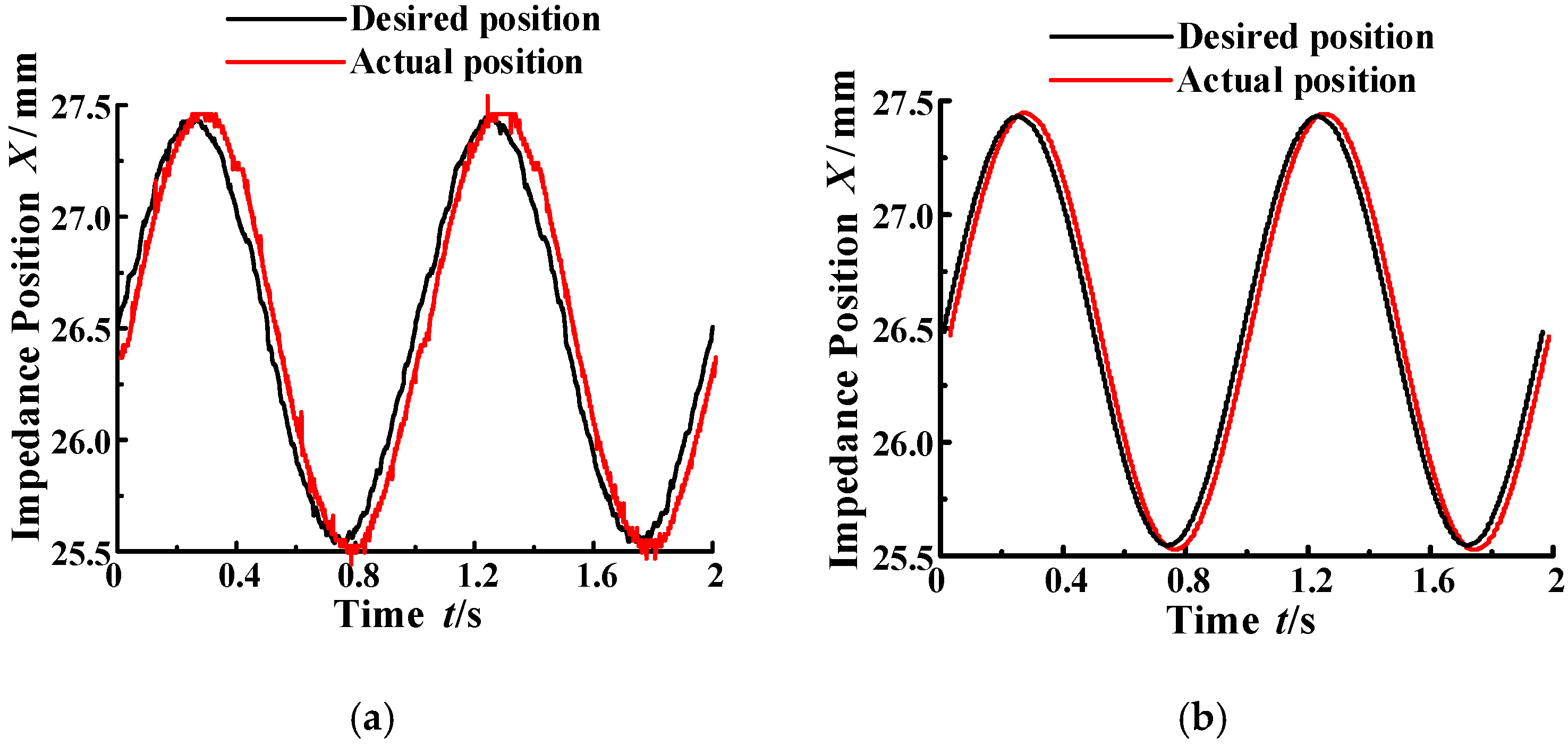
In a position-based impedance control system, the load acts as an external disturbance force that is simulated by the force-based control system. Thus, the desired position can be defined as the ratio of the actual force to the desired impedance characteristic , i.e., the ratio of the value of the force sensor to . The actual position is the output of the system to be tested, i.e., the value of the position sensor. The experimental and simulation curves of the sinusoidal response are shown in Figure 8, Figure 9, Figure 10 and Figure 11 in sequence of working conditions [17].
The mean values of performance indexes in different conditions are shown in Table 3.
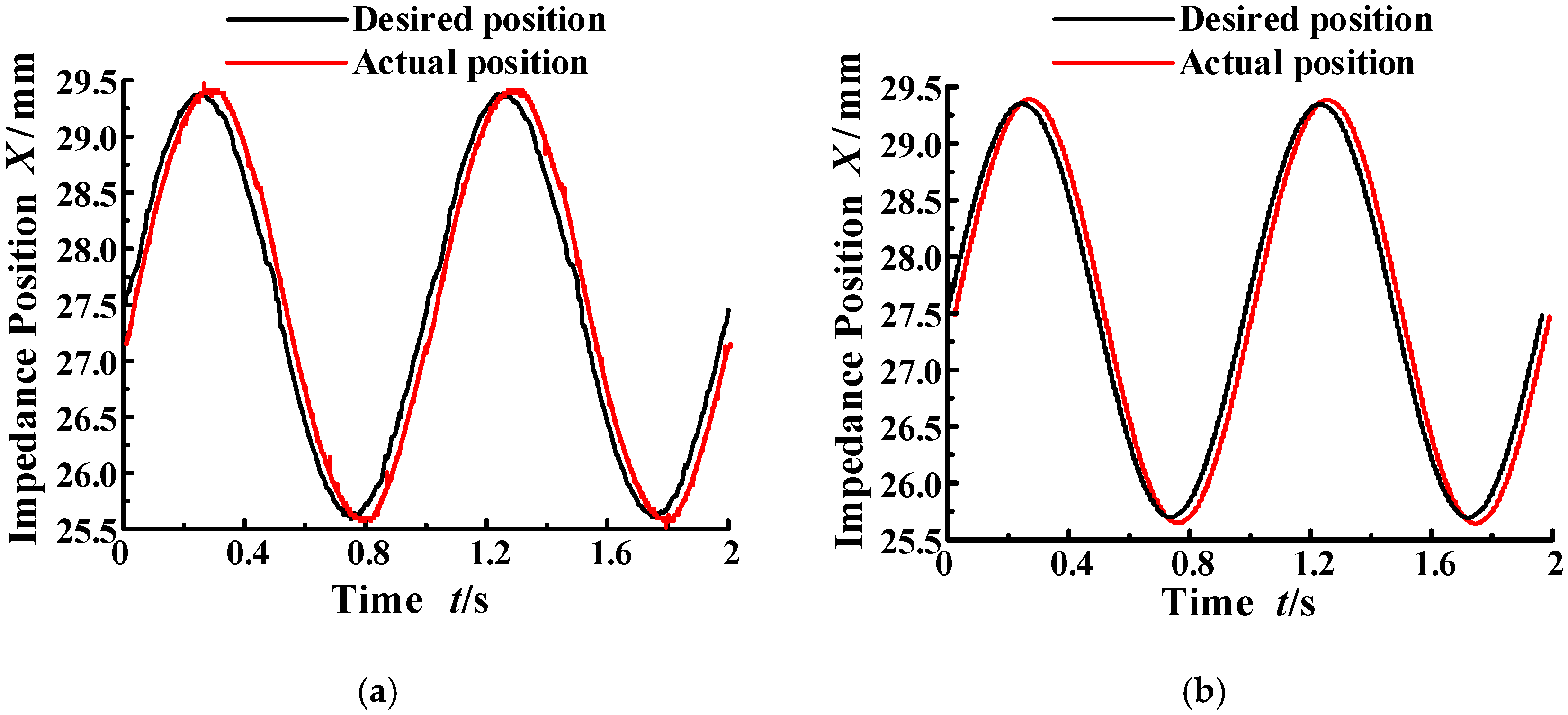
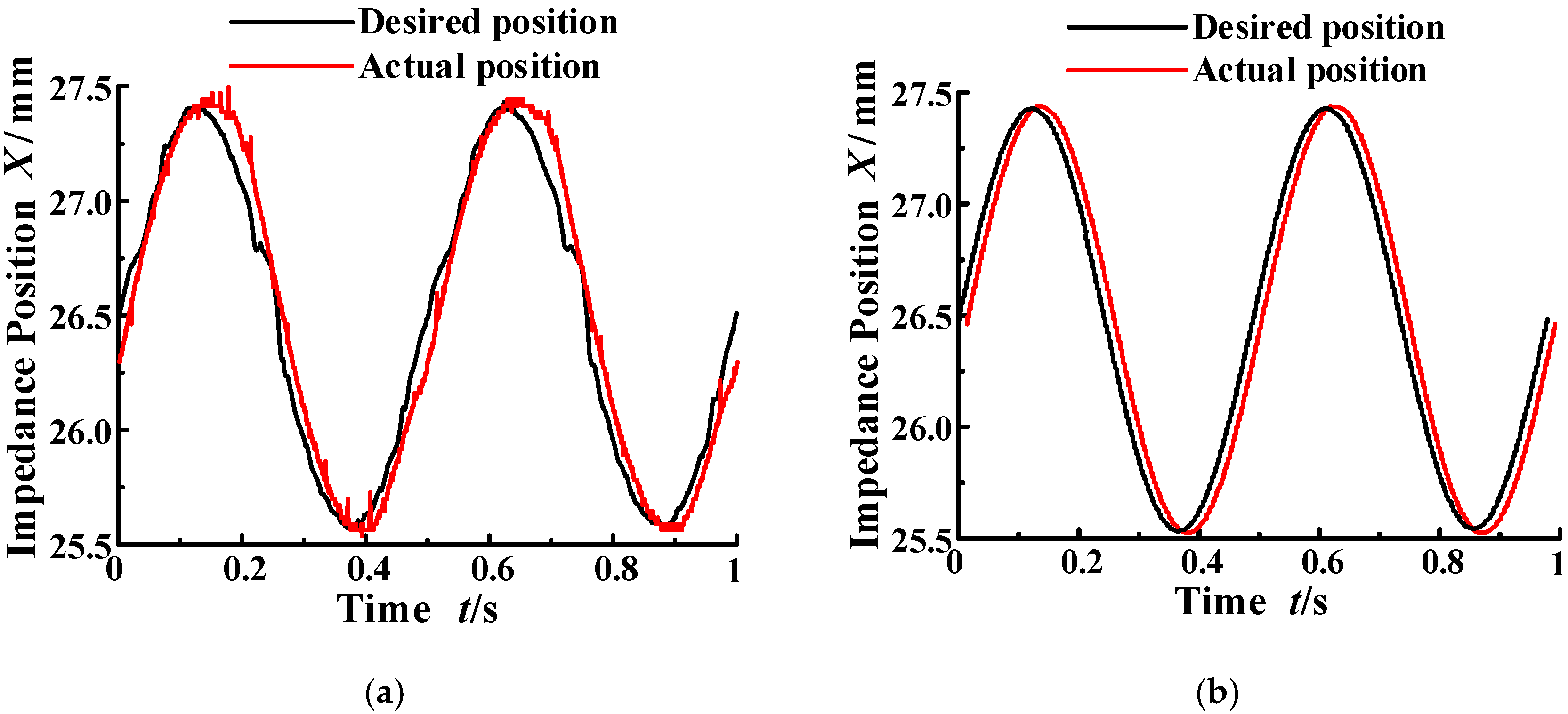
As it can be seen in Table 3, the values of the two performance indexes are close in experiment and simulation, which indicates that the experimental curves fit the simulation curves well. As the position-based impedance control theory in Figure 8 shows, the actual position is greater than the desired one. Thus, the amplitude attenuation is a negative value. It increases with the increase of the disturbance force’s amplitude, but has few relationships with the frequency. In contrast, the phase angle delay increases with the frequency, but has few relationships with the amplitude.
4. Methods of Sensitivity Analysis
4.1. Contrast between First-Order and Second-Order Sensitivity Analysis
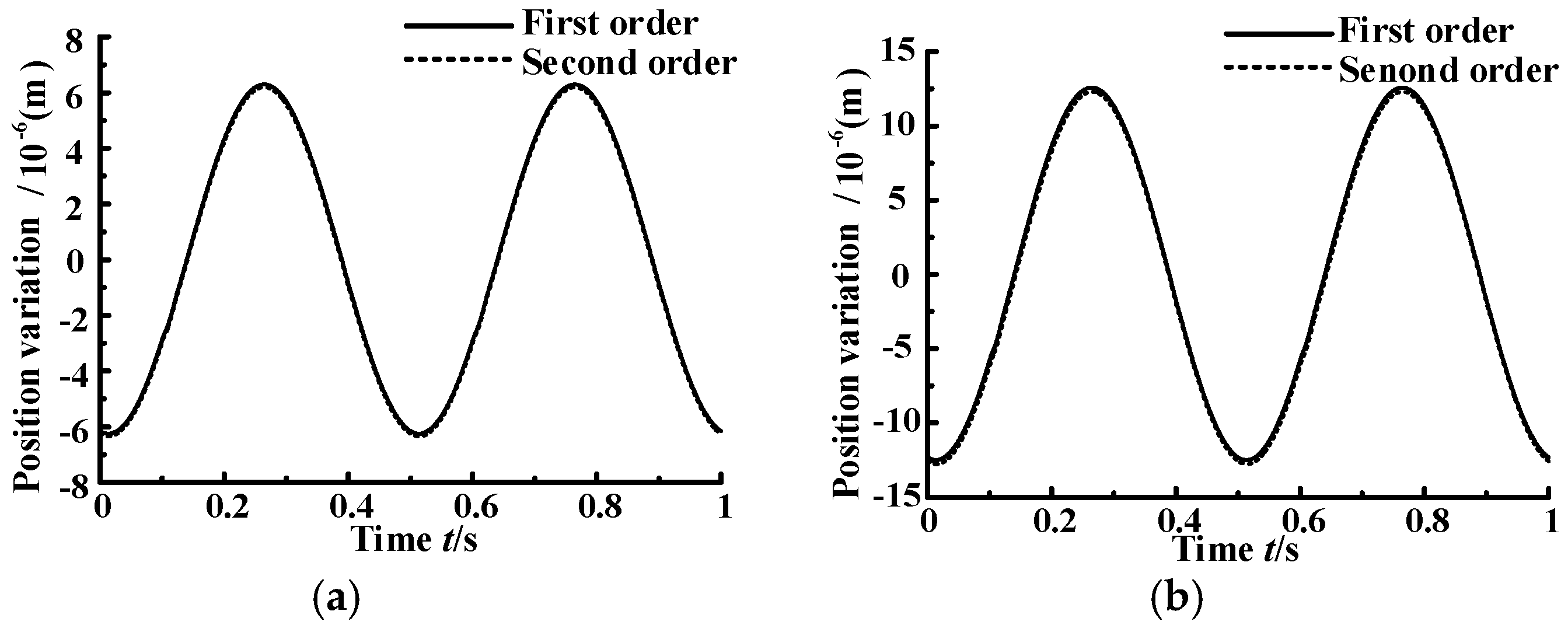
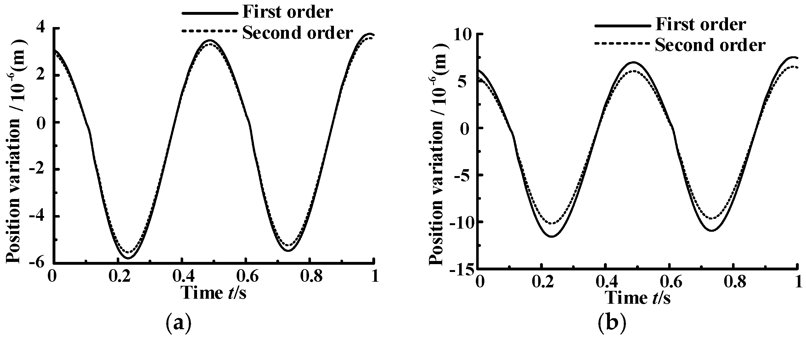
Desired stiffness and desired damping are control parameters of the impedance control outer loop. Proportional gain and integral gain are control parameters of the position control inner loop. They affect the impedance control performance in different ways. So, in this paper, the system output position is mainly discussed, which is influenced by the variation of the four parameters. Because of space limitations, only one working condition (bias: 1500 N, amplitude: 1000 N, frequency: 2 Hz) is studied. The first-order and second-order trajectory sensitivity analysis methods researched in our previous works [15,16] are adopted to analyze the position variation when the four parameters increase 10% to 20%. The contrast curves are shown in Figure 12, Figure 13, Figure 14 and Figure 15.
The following conclusions can be reached from the four sets of curves. There is little difference between the first-order position variation and the second-order variation when the values of the four parameters increases 10%. Specifically, the curves of desired damping and integral gain almost overlap. In the other two sets, the maximum error is no more than 10% of the amplitude. When the values of the four parameters increase 20%, the variations of first-order and second-order are still close, although there is some increase of their error. Specifically, for desired damping and integral gain , the variation curves of first-order and second-order are still close. As for the proportional gain , its maximum error is no more than 10% of the amplitude. When it comes to the desired stiffness , its maximum error is no more than 20% of the amplitude.
The method of second-order trajectory sensitivity analysis has a very high accuracy, while its calculation is complicated and demands a lot of hard work. Particularly in this paper, when the four parameters increase less than 20%, the corresponding results of the first-order and second order sensitivity analysis method are close. So, in order to ensure the simplicity of calculation and application, the method of first-order sensitivity analysis is adopted to analyze the sensitivity of the four parameters under different working conditions.
The method studied previously can precisely analyze the sensitivity of the parameters. Compared with the second-order method, the calculation has been largely simplified under the method of first-order trajectory sensitivity analysis, but it also requires solving first-order linear non-homogeneous differential equations with time-varying factors, which makes the program complicated. So, in order to ensure high solving accuracy, a new method with an easier calculation is proposed. That is the first-order matrix sensitivity analysis.
4.2. Deduction of First-Order Matrix Sensitivity Analysis Theory
Combined with the position-based impedance control method, the equation of the HDU system can be expressed as follows:
where is m−dimensional state vector, is r−dimensional vector unrelated to , is p−dimensional vector, and t is time.
The initial value of the state vector can be obtained by giving the initial value of the input vector and the initial value of parameter vector , and the initial state of the equations is:
where the variation of parameter vector and input vector can change the value of , the error of the state variable , which is expressed as follows:
Expanded in the form of the first-order Taylor Series, Equation (9) can be expressed as follows:
If we bring Equation (12) into Equation (14) and ignore the higher-order terms, then we can get:
Equation (15) can also be expressed as follows:
In Equation (17), supposing:
where is order matrix, and the n-th line indicates the relation among the n-th state variable .
In Equation (17), supposing:
where, is the order matrix, the n-th line indicates the relation among the n-th state variable and p parameter vectors. Bring Equations (17) and (18) into Equation (16), then:
Equation (19) is an approximate expression of resulted from the change of parameter vector and input vector , in which indicates an order parameter sensitivity matrix of parameter vector with time-varying factors. indicates an order input sensitivity matrix of input vector with time-varying factors.
When taking no account of the variation of input vector, Equation (19) can be simplified as follows:
The output equation of the system can be expressed as follows:
where and are matrices of output equation factors. The change of output variable resulting from the parameter variation can be reached after solving parameter sensitivity matrix .
5. Dynamic Sensitivity Analysis
5.1. Contrast between Two Analysis Method of First-Order Sensitivity
The state vectors’ initial values of the servo-cylinder’s position, velocity, and pressure of two chambers, the servo-valve’s position, velocity and acceleration are zero. So, the initial value of parameter sensitivity matrix can be expressed as follows:
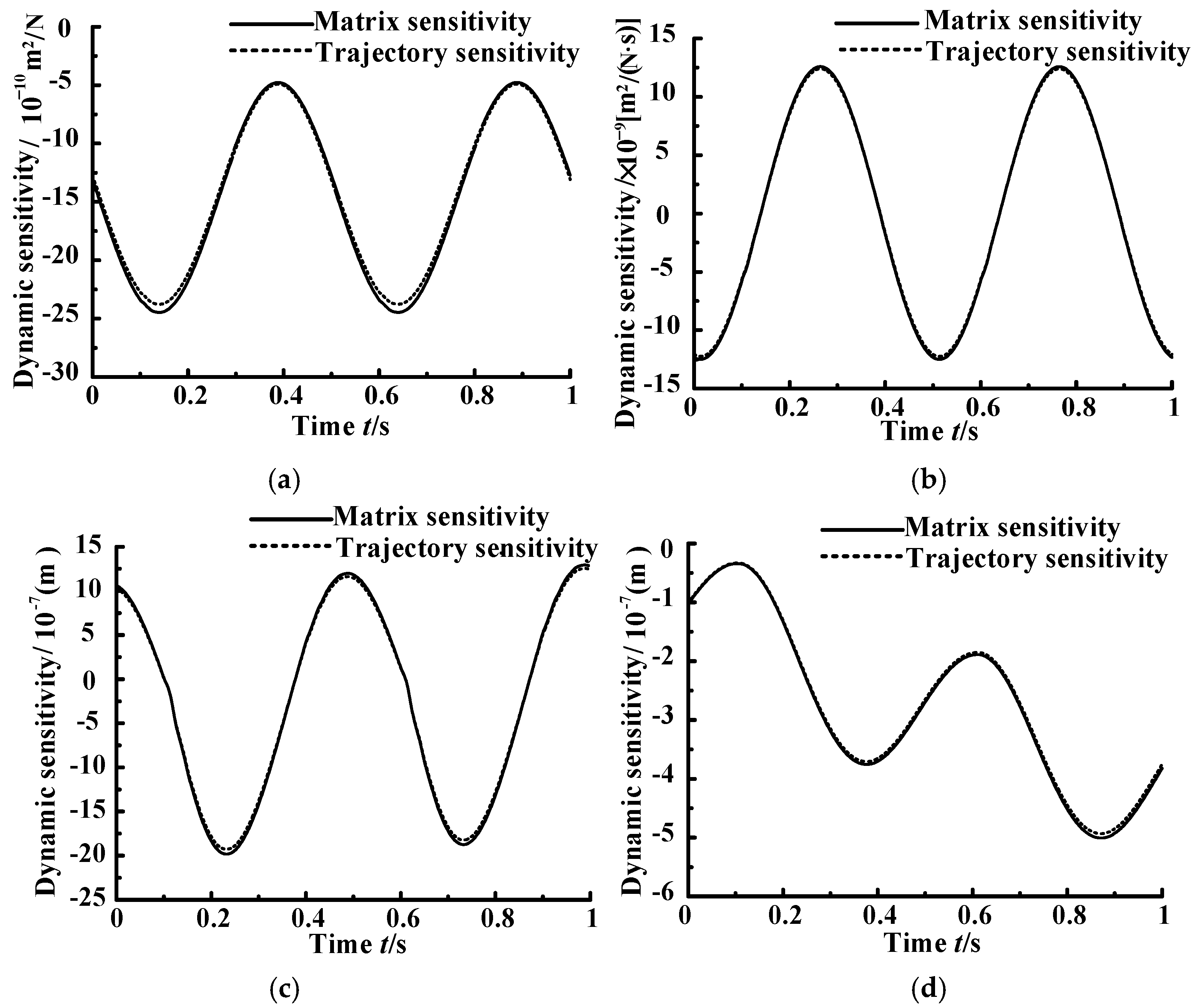
Solve the sensitivity matrices in MATLAB, and then compare the results from the trajectory sensitivity in Section 3.1 and , the inverse value of the control parameter’s sensitivity matrix of the system output position. Due to space limitations, only one working condition (1500 N bias, 1000 N amplitude, 2 Hz frequency) is shown. The curves of parameter dynamic sensitivity in this situation is shown in Figure 16.
It can be seen that the dynamic compliance curves of first-order matrix sensitivity deviate little from the curves of first-order trajectory sensitivity. Particularly, by comparing Figure 12, Figure 13, Figure 14 and Figure 15 in Section 3.1, it can be found that the value calculated by first-order matrix sensitivity is more approximate to the result of second-order trajectory sensitivity and has higher precision than first-order trajectory sensitivity. Moreover, only a two-dimension matrix calculation is needed, which avoids solving complicated differential equations with time-varying factors. So, in the research field of this paper, the first-order matrix sensitivity analysis method is more adapted than the first-order trajectory sensitivity analysis method. Whether calculating a high-order and multi-dimensional matrix is easier than solving differential equations with time-varying factors cannot be determined, so it requires further research to find which is better between the high-order matrix sensitivity analysis method and the high-order trajectory sensitivity analysis method. However, due to space constraints, this will not be discussed in this paper.
5.2. Contrast of Dynamic Sensitivity Analysis in Each Working Condition
For the convenience of contrast, the variation of system position response when each parameter increases 10% is calculated according to Equation (21). The curves of position variation with time is shown in Figure 17.
As it can be seen in Figure 17:
- The variation of each parameter affects impedance control position output. The position varies periodically with the sinusoidal disturbance force. Among the parameters, the desired stiffness affects the output position much more than the others. The influence from integral gain is the most irrelevant. Desired damping and proportional gain have similar influences on the output position. With the disturbance force in sinusoidal variation, varies by following the curve of minus cosine, and varies by following the curve of cosine.
- The order of magnitudes of output position increases with the increase of sinusoidal disturbance force. However, there isn’t an obvious relationship between the effects on output position and the frequency of the disturbance force.
Using the method of dynamic sensitivity analysis, the qualitative effects on impedance control performance is analyzed. In order to analyze the effects on main system performance indexes and the varying patterns of parameter sensitivity under different working conditions, a quantificational analysis is needed.
6. Sensitivity Quantitative Analysis
6.1. Sensitivity Indexes
Two measurement indexes are introduced to analyze the effects on main performance indexes resulting from the variation of parameters in different working conditions.
For sinusoidal response, in a stable sinusoidal period, the variation of parameters results in the change of the output position amplitude. The mean of amplitude attenuation is defined as the first sensitivity measurement index , which is expressed as follows:
where,
Similarly, for phase angle delay, another important index, its mean is defined as the second sensitivity measurement index , which is expressed as follows:
where,
Using the above two indexes, and , the effect on output position resulting from the variation of parameters can be quantificationally analyzed.
6.2. Sensitivity Histograms in Different Working Conditions
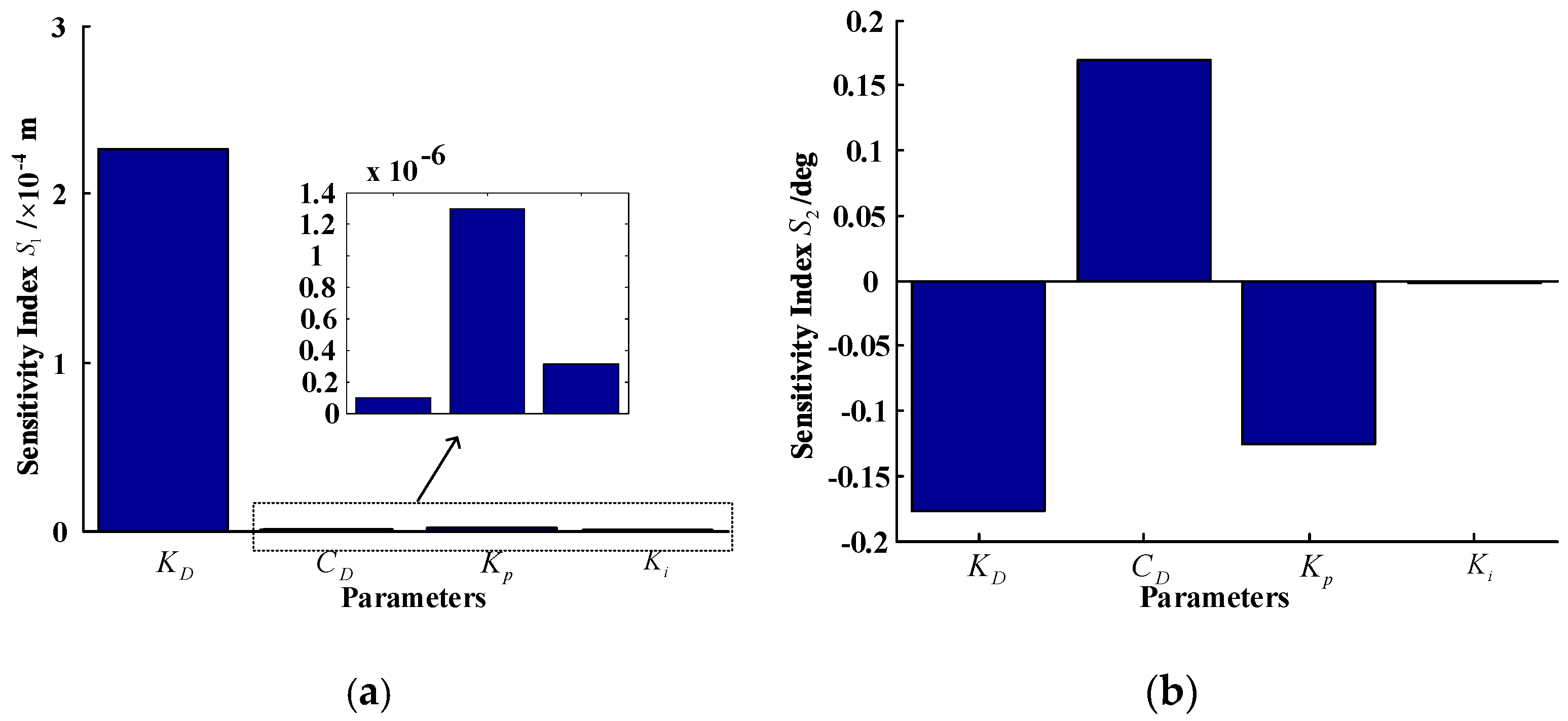
According to Equations (23)–(27), the two sensitivity histograms are shown in Figure 18, Figure 19, Figure 20 and Figure 21, when the four control parameters increase 10% in four working conditions.
- In all conditions, is a positive value, so the increase of the four parameters will result in the reduction of the position amplitude attenuation. The of desired stiffness is much greater than the other parameters, which illustrates that the variation of has a remarkable influence on output position amplitude attenuation, and more relation with disturbance force amplitude than the disturbance force frequency. Under the first working condition, amplitude attenuation reduced about 0.2 mm when increased 10%. The of proportional gain is greater than that of and . The of and have some correlation with disturbance force amplitude, but have little correlation with disturbance force frequency.
- The of the four control parameters has positive or negative values in different conditions. An increase of the parameters has different influences on the phase angle delay of the output position. Specifically, having more relation with disturbance force frequency than the amplitude, the of and have nearly the same absolute value, but an opposite sign. Their increase has totally different influences on phase angle delay. An approximate 10% increase of them generates about 0.18° of phase angle delay error. The of has correlation with both disturbance force amplitude and frequency. The larger the frequency, the more remarkable the influence on phase delay. The of is close to the of . The of is about 0.001° on magnitude order, much less than the other control parameters.
7. Experiment
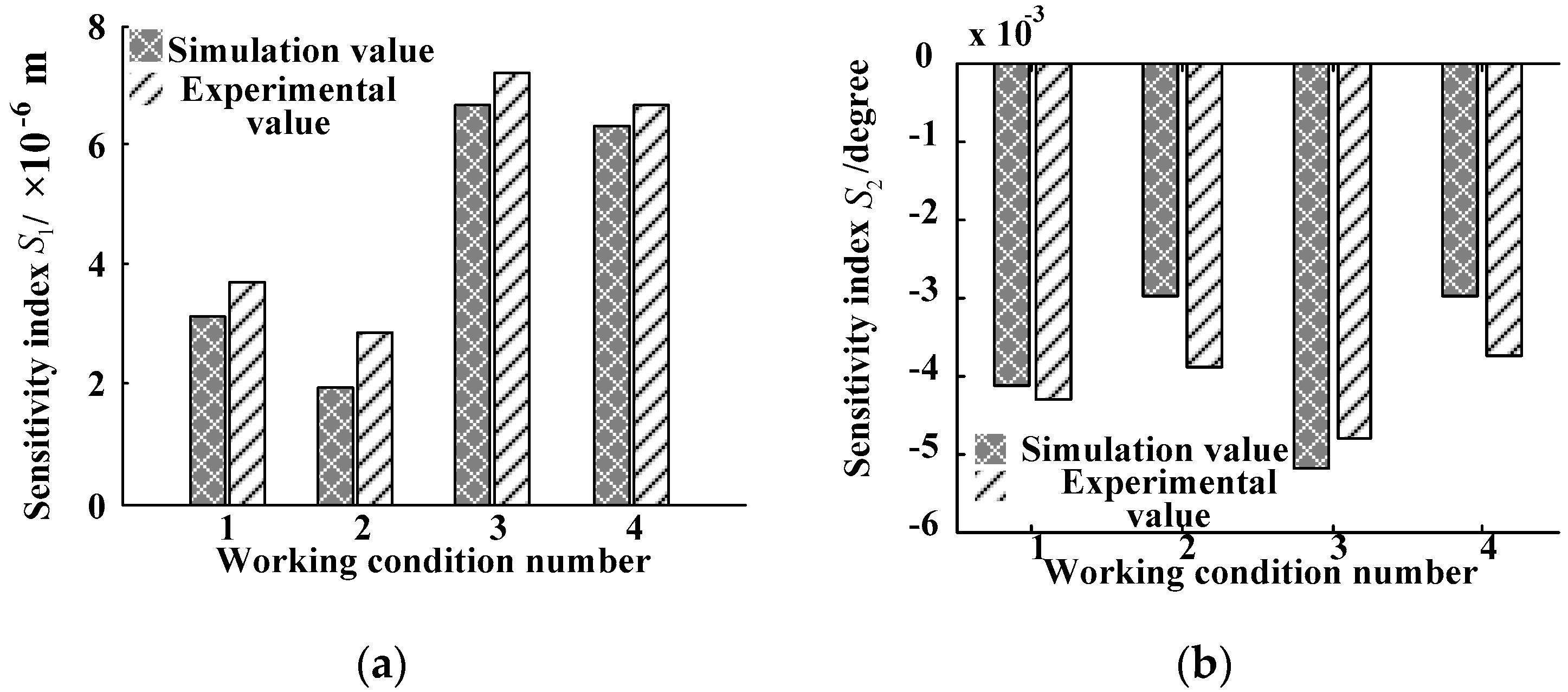
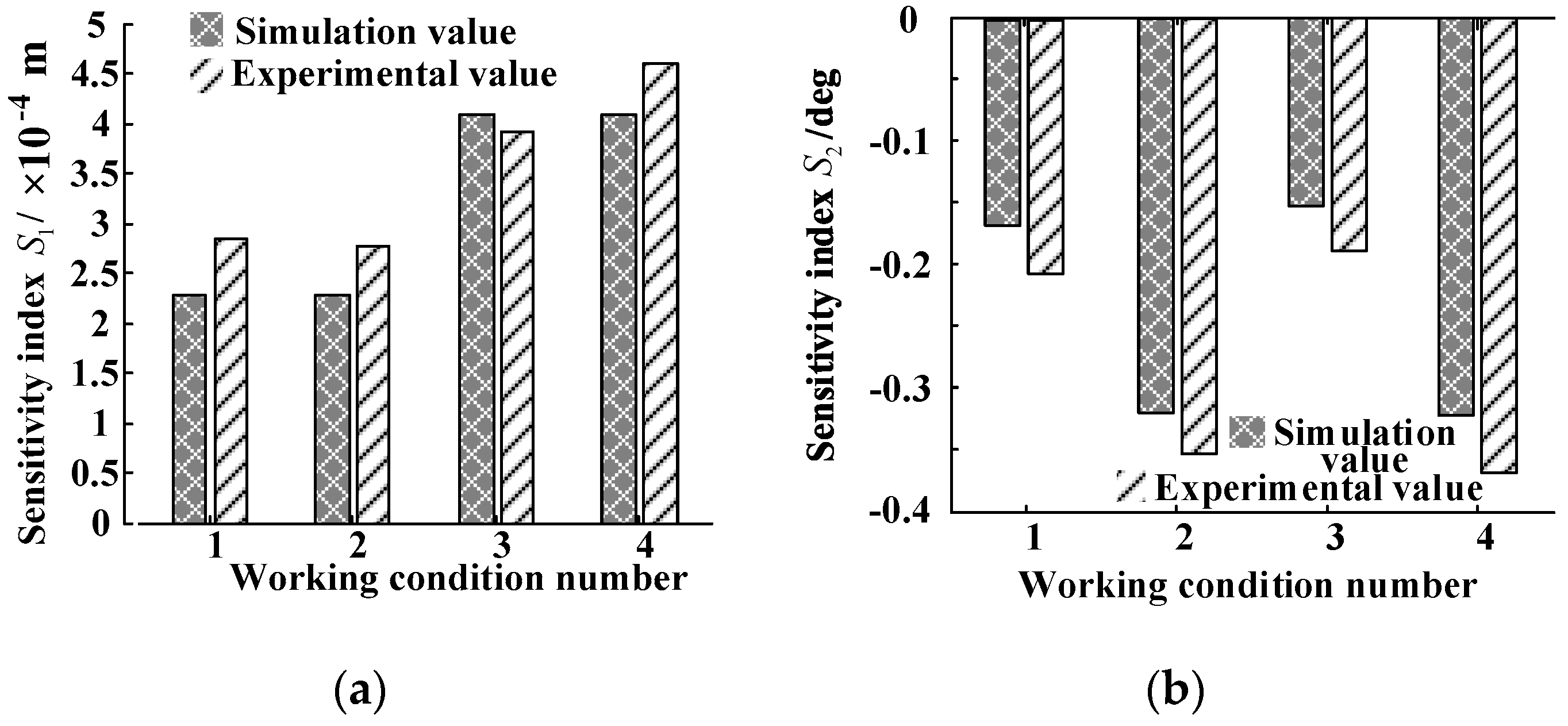
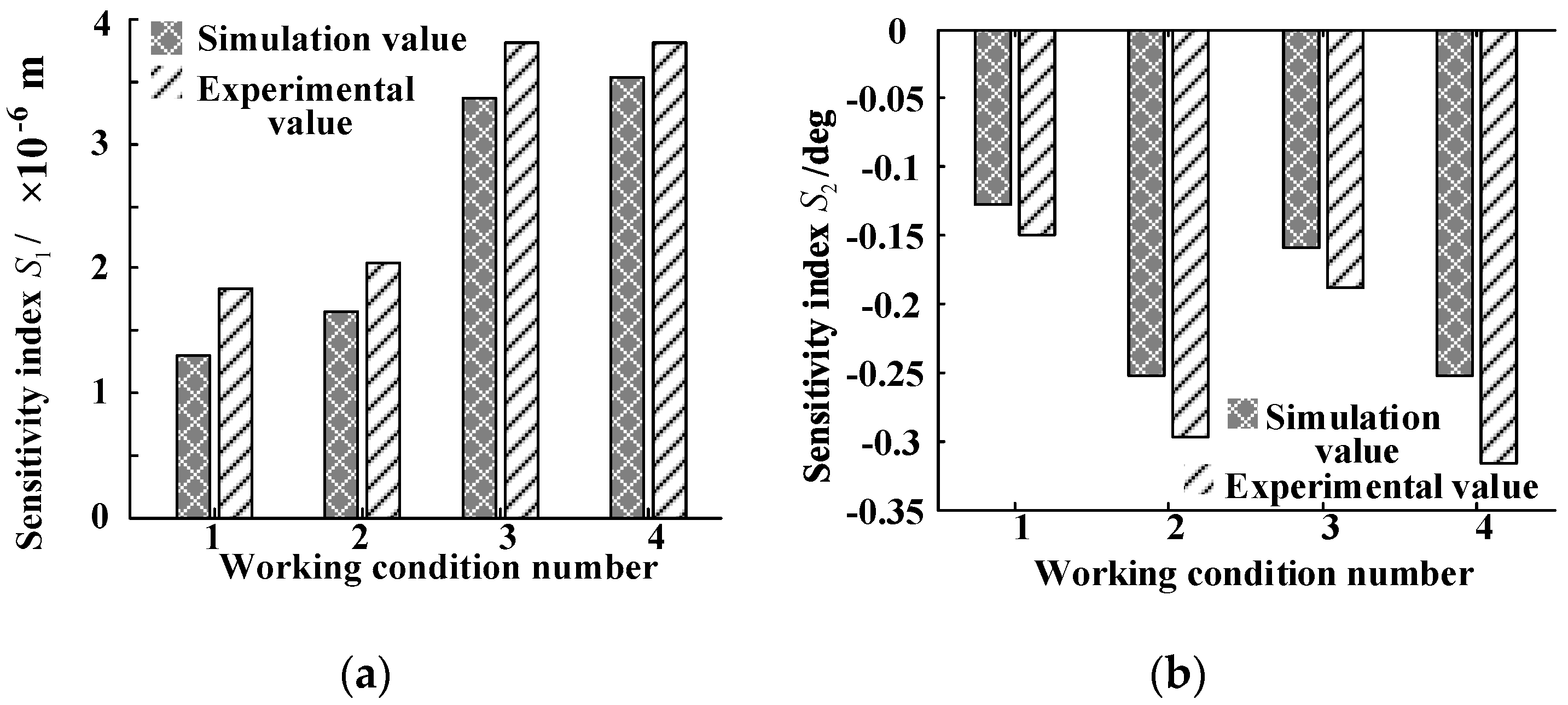
Compared with structural parameters and some working parameters, control parameters can change and be measured during the working process. The two sensitivity indexes of four control parameters are studied by experiments in this section. The mean of several samples is included to ensure the accuracy of the experiment. By comparing the measured data and the simulation result of the first-order sensitivity matrix, the contrast histograms of experiment value and simulation value for the two sensitivity indexes when the four parameters increase 10% under four working conditions are shown in Figure 22, Figure 23, Figure 24 and Figure 25.
In Figure 22, Figure 23, Figure 24 and Figure 25, the maximum and mean errors between the experimental value and the simulation value are shown in Table 4.
According to Figure 22, Figure 23, Figure 24 and Figure 25 and Table 4, the experimental value and simulation value have the same magnitude and similar variation patterns. Except that the maximum errors of of and are above 30%, the others are less than 20%. The mean errors of the four parameters are less than 16%. For , the maximum error is about 20%. Except that mean error of for is 16%, the others’ mean errors are about 10%.
8. Conclusions
In this paper, a HDU position-based impedance control method is proposed. The method of sensitivity analysis is selected in research. Dynamic sensitivity analysis and quantificational sensitivity analysis are conducted to study the four main control parameters. The results from the research are verified by experiments. Here are the conclusions summarized in this paper:
- Sensitivity analysis method is used to analyze the four parameters, which are the proportional gain and integral gain of the inner loop PID controller, and the desired stiffness and desired damping of the impedance outer loop. The first-order and second-order effects on position are analyzed by the trajectory sensitivity analysis, when the four parameters increase no more than 20%. In spite of its higher accuracy, the second-order sensitivity analysis requires a complex solving process with lots of hard work. Considering that the largest error between the first-order and second-order sensitivity analysis methods is below 20% of the amplitude, this paper proposed the easier first-order matrix sensitivity analysis method. Compared with first-order trajectory sensitivity, the first-order matrix sensitivity method is simpler and more accurate in computing.
- The effects of parameter variation on output position varies periodically with sinusoidal disturbance force. Among the parameters, desired stiffness affects the output position much more than the other parameters. The influence of integral gain is the least. Desired damping and proportional gain have a similar influence on the output position.
- The of each parameter is a positive value, which shows that the increase of the four parameters will result in the reduction of the position amplitude attenuation. The of each parameter has positive or negative values in different conditions. Their increase has different influences on the phase angle delay of output positions.
Acknowledgments
The project is supported by National Natural Science Foundation of China (Grant No. 51605417), Key Project of Hebei Province Natural Science Foundation (Grant No. E2016203264).
Author Contributions
B.Y. designed the experiments; K.B. wrote the paper; X.K. conceived the research idea; Z.G. performed the experiments; G.M. and W.L. analyzed the data.
Conflicts of Interest
The founding sponsors had no role in the design of the study; in the collection, analyses, or interpretation of data; in the writing of the manuscript, and in the decision to publish the results.
References
- Montes, H.; Armada, M. Force Control Strategies in Hydraulically Actuated Legged Robots. Int. J. Adv. Robot. Syst. 2016, 13, 50. [Google Scholar] [CrossRef]
- Nabulsi, S.; Sarria, J.; Montes, H.; Armada, M. High Resolution Indirect Feet-Ground Interactions Measurement for Hydraulic Legged Robots. J. IEEE Trans. Instrum. Meas. 2009, 58, 3396–3404. [Google Scholar] [CrossRef]
- Huang, Q.; Oka, K. Phased compliance control with virtual force for six-legged walking robot. Int. J. Innov. Comput. Inf. Control 2008, 4, 3359–3373. [Google Scholar]
- Kong, X.D.; Ba, K.X.; Yu, B.; Cao, Y.; Zhu, Q.; Zhao, H. Research on the force control compensation method with variable load stiffness and damping of the hydraulic drive unit force. Chin. J. Mech. Eng. (English Ed.) 2016, 29, 454–464. [Google Scholar] [CrossRef]
- Ba, K.X.; Yu, B.; Kong, X.D.; Zhao, H.-L.; Zhao, J.-S.; Zhu, Q.-X.; Li, C.-H. The dynamic compliance and its compensation control research of the highly integrated valve-controlled cylinder position control system. Int. J. Control Autom. Syst. 2017, 15, 1814–1825. [Google Scholar] [CrossRef]
- Li, M.T.; Jiang, Z.Y.; Wang, P.F.; Sun, L.N.; Ge, S.S. Control of a Quadruped Robot with Bionic Springy Legs in Trotting Gait. J. Bionic Eng. 2014, 11, 188–198. [Google Scholar] [CrossRef]
- Kimura, H.; Fukuoka, Y.; Cohen, A.H. Adaptive dynamic walking of a quadruped robot on natural ground based on biological concepts. Int. J. Robot. Res. 2007, 26, 475–490. [Google Scholar] [CrossRef]
- Poulakakis, I.; Smith, J.A.; Buehler, M. Modeling and experiments of untethered quadrupedal running with a bounding gait: The scout ii robot. Int. J. Robot. Res. 2005, 24, 239–256. [Google Scholar] [CrossRef]
- Seok, S.; Wang, A.; Meng, Y.C.; Otten, D. Design principles for highly efficient quadrupeds and implementation on the MIT Cheetah robot. In Proceedings of the IEEE International Conference on Robotics and Automation, Karlsruhe, Germany, 6–10 May 2013; IEEE: Piscataway, NJ, USA, 2013; pp. 3307–3312. [Google Scholar]
- Playter, R.; Buehler, M.; Raibert, M. BigDog. In Unmanned Systems Technology VIII, Proceedings of SPIE; SPIE: Bellingham, WA, USA, 2006; Volume 6230, pp. 1–6. [Google Scholar]
- Semini, C.; Barasuol, V.; Boaventura, T.; Frigerio, M.; Focchi, M. Towards versatile legged robots through active impedance control. Int. J. Robot. Res. 2015, 34, 1003–1020. [Google Scholar] [CrossRef]
- Rong, X.; Li, Y.; Ruan, J.; Li, B. Design and simulation for a hydraulic actuated quadruped robot. J. Mech. Sci. Technol. 2012, 26, 1171–1177. [Google Scholar] [CrossRef]
- Vilenus, M. The Application of Sensitivity Analysis to Electrohydraulic Position Control Servos. J. Dyn. Syst. Meas. Control 1983, 105, 77–82. [Google Scholar] [CrossRef]
- Farasat, S.; Ajam, H. Sensitivity Analysis of Parameter Changes in Nonlinear Hydraulic Control Systems. Int. J. Eng. 2005, 18, 239–252. [Google Scholar]
- Kong, X.D.; Yu, B.; Quan, L.; Ba, K.; Wu, L. Nonlinear Mathematical Modeling and Sensitivity Analysis of Hydraulic Drive Unit. Chin. J. Mech. Eng. 2015, 28, 999–1011. [Google Scholar] [CrossRef]
- Kong, X.D.; Ba, K.X.; Yu, B.; Quan, L.; Wu, L. Trajectory Sensitivity Analysis of First Order and Second Order on Position Control System of Highly Integrated Valve−controlled Cylinder. J. Mech. Sci. Technol. 2015, 29, 4445–4464. [Google Scholar] [CrossRef]
- Kong, X.; Zhao, H.; Li, B.W.; Ba, K. Analysis of position-based impedance control method and the composition of system dynamic compliance. In Proceedings of the IEEE International Conference on Aircraft Utility Systems (AUS), Beijing, China, 10–12 October 2016; pp. 454–459. [Google Scholar]
Figure 1.
The quadruped robot prototype, single leg and hydraulic drive unit (HDU) performance test platform. (a) Quadruped robot prototype; (b) Single leg; (c) HDU.
Figure 1.
The quadruped robot prototype, single leg and hydraulic drive unit (HDU) performance test platform. (a) Quadruped robot prototype; (b) Single leg; (c) HDU.

Figure 2.
Schematic of HDU performance test platform.

Figure 3.
Composition of HDU performance test platform. (a) HDU performance test platform; (b) dSPACE controller.
Figure 3.
Composition of HDU performance test platform. (a) HDU performance test platform; (b) dSPACE controller.
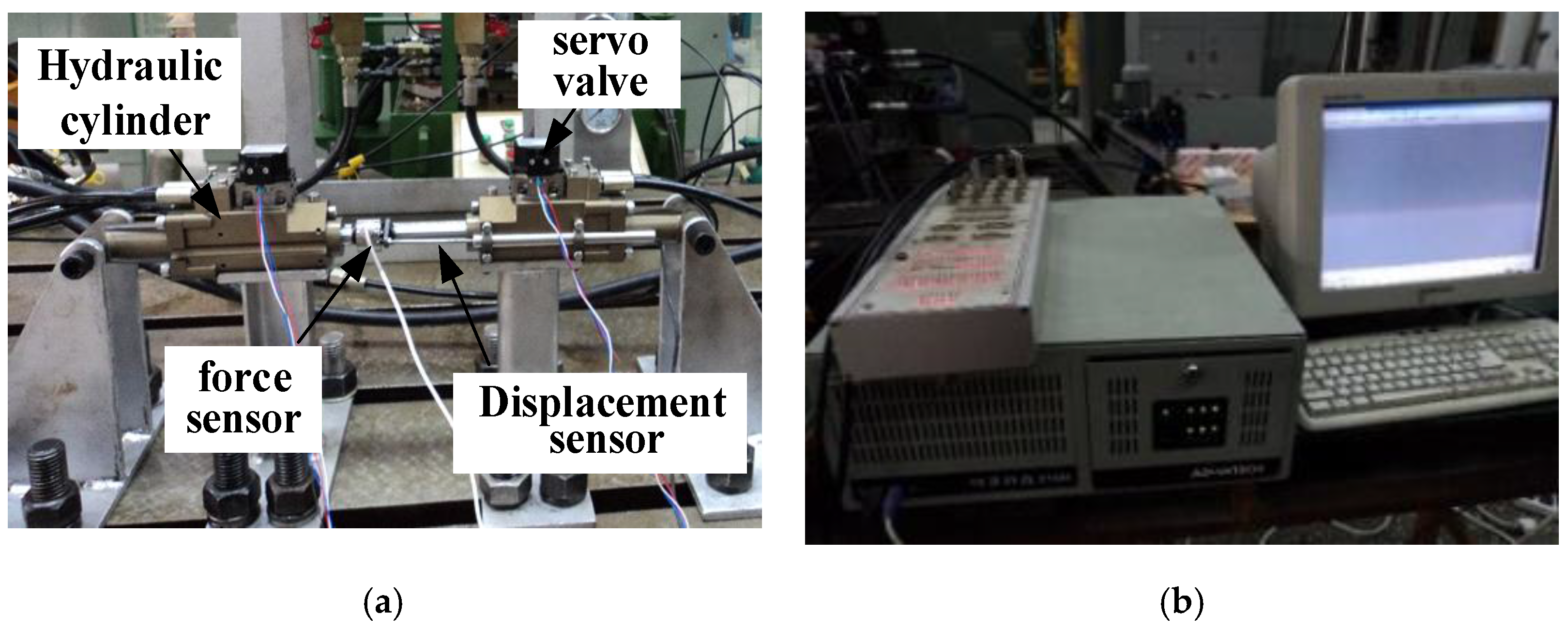
Figure 4.
Force schematic of the load.
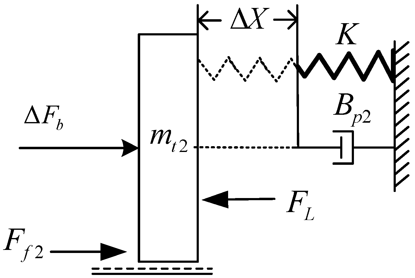
Figure 5.
Force schematic of HDU.

Figure 6.
Position-based impedance control schematic.

Figure 7.
Block diagram of HDU position-based impedance control.

Figure 8.
Experimental and simulation curves of sinusoidal response (frequency: 1 Hz, bias: 1500 N, amplitude: 1000 N). (a) Experimental curves; (b) Simulation curves.
Figure 8.
Experimental and simulation curves of sinusoidal response (frequency: 1 Hz, bias: 1500 N, amplitude: 1000 N). (a) Experimental curves; (b) Simulation curves.

Figure 9.
Experimental and simulation curves of sinusoidal response (frequency: 1 Hz, bias: 2500 N, amplitude: 2000 N). (a) Experimental curves; (b) Simulation curves.
Figure 9.
Experimental and simulation curves of sinusoidal response (frequency: 1 Hz, bias: 2500 N, amplitude: 2000 N). (a) Experimental curves; (b) Simulation curves.

Figure 10.
Experimental and simulation curves of sinusoidal response (frequency: 2 Hz, bias: 1500 N, amplitude: 1000 N). (a) Experimental curves; (b) Simulation curves.
Figure 10.
Experimental and simulation curves of sinusoidal response (frequency: 2 Hz, bias: 1500 N, amplitude: 1000 N). (a) Experimental curves; (b) Simulation curves.

Figure 11.
Experimental and simulation curves of sinusoidal response (frequency: 2 Hz, bias: 2500 N, amplitude: 2000 N). (a) Experimental curves; (b) Simulation curves.
Figure 11.
Experimental and simulation curves of sinusoidal response (frequency: 2 Hz, bias: 2500 N, amplitude: 2000 N). (a) Experimental curves; (b) Simulation curves.
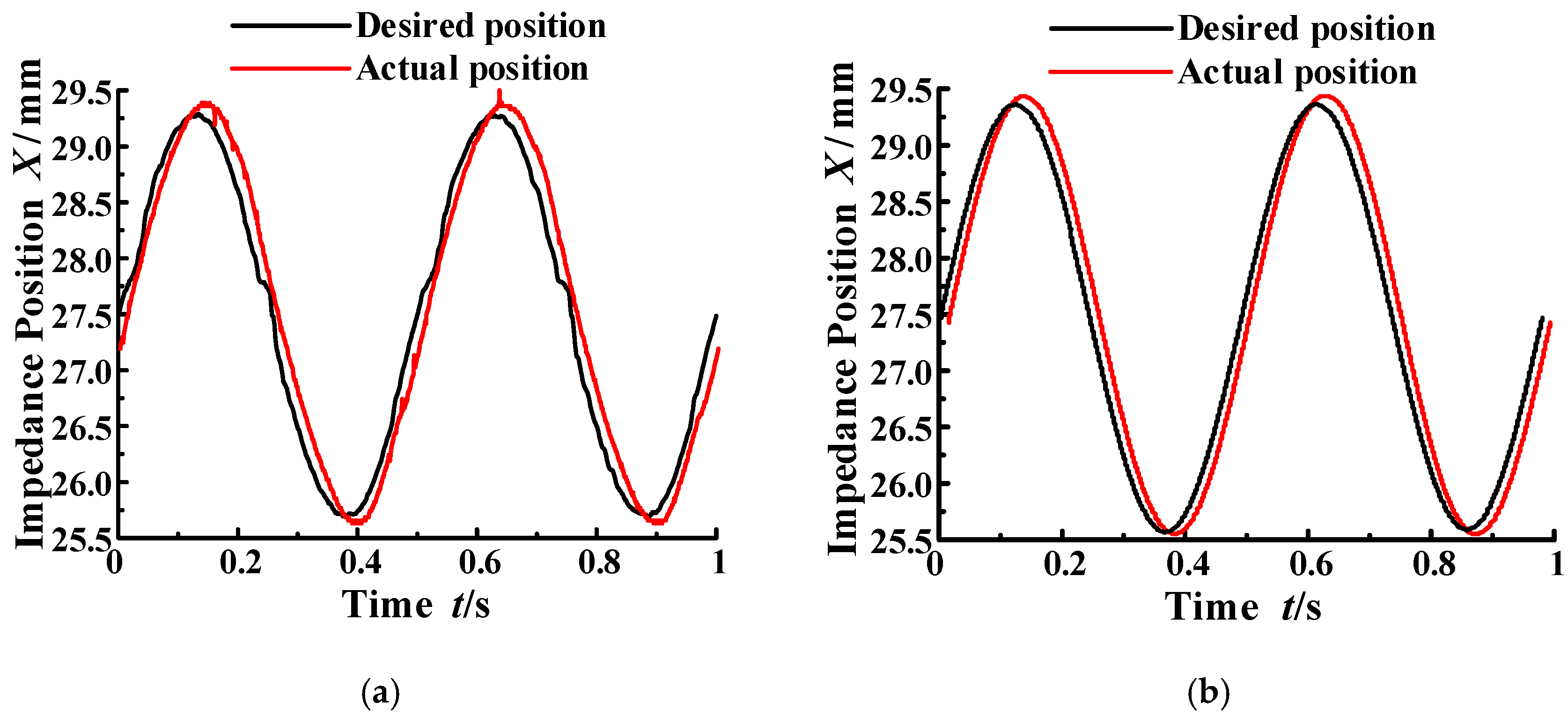
Figure 12.
Position variation resulting from variation. (a) Four parameters increase 10%; (b) Four parameters increase 20%.
Figure 12.
Position variation resulting from variation. (a) Four parameters increase 10%; (b) Four parameters increase 20%.
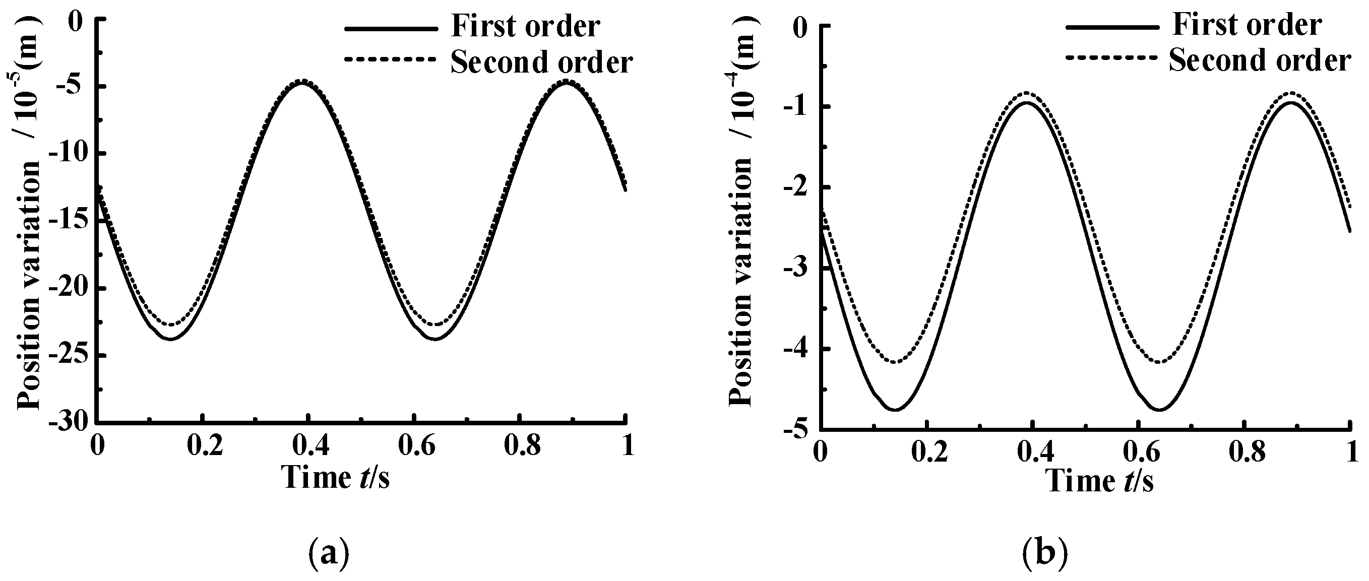
Figure 13.
Position variation resulting from variation. (a) Four parameters increase 10%; (b) Four parameters increase 20%.
Figure 13.
Position variation resulting from variation. (a) Four parameters increase 10%; (b) Four parameters increase 20%.

Figure 14.
Position variation resulting from variation. (a) Four parameters increase 10%; (b) Four parameters increase 20%.
Figure 14.
Position variation resulting from variation. (a) Four parameters increase 10%; (b) Four parameters increase 20%.

Figure 15.
Position variation resulting from variation. (a) Four parameters increase 10%; (b) Four parameters increase 20%.
Figure 15.
Position variation resulting from variation. (a) Four parameters increase 10%; (b) Four parameters increase 20%.
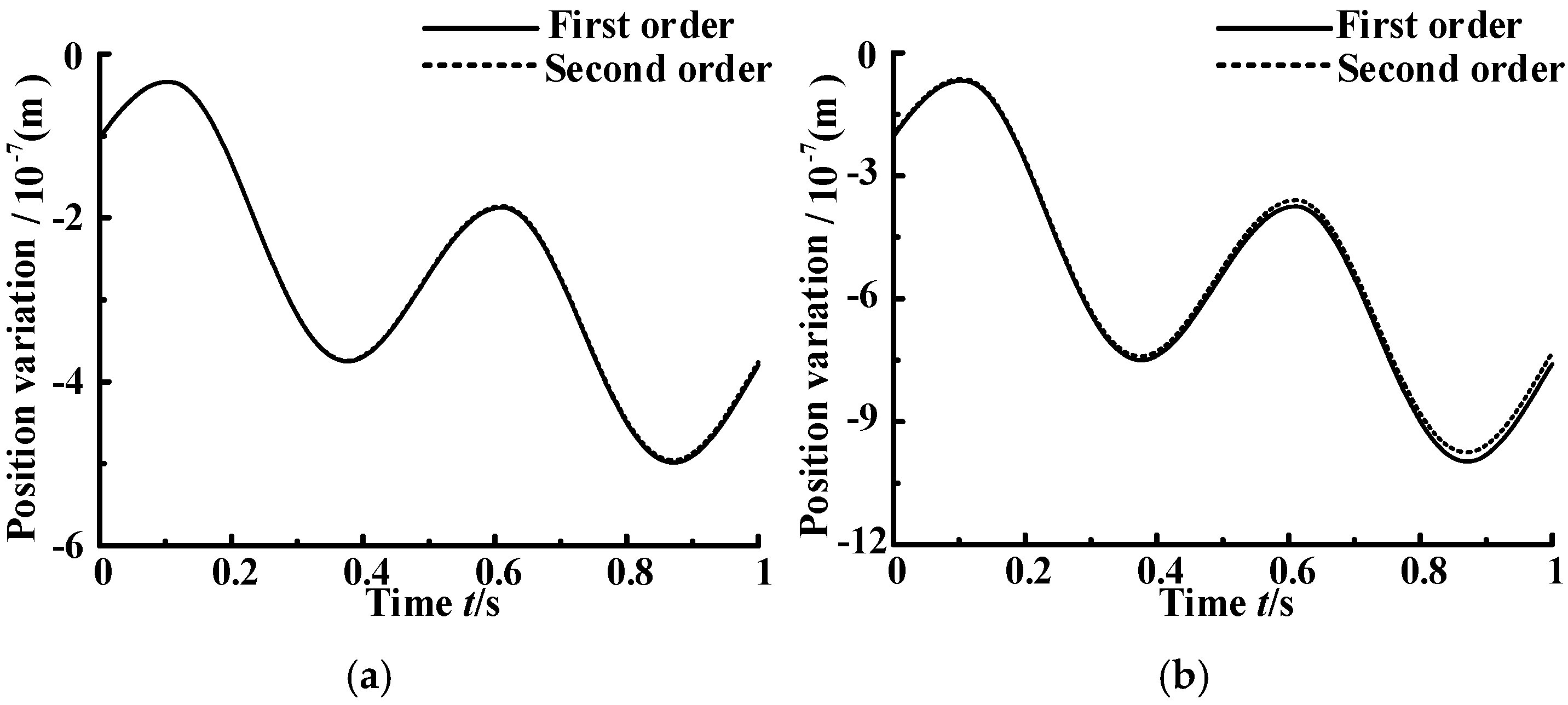
Figure 16.
The curves of dynamic sensitivity between two sensitivity methods. (a) First-order dynamic sensitivity of ; (b) First-order dynamic sensitivity of ; (c) First-order dynamic sensitivity of ; (d) First-order dynamic sensitivity of .
Figure 16.
The curves of dynamic sensitivity between two sensitivity methods. (a) First-order dynamic sensitivity of ; (b) First-order dynamic sensitivity of ; (c) First-order dynamic sensitivity of ; (d) First-order dynamic sensitivity of .

Figure 17.
Variation of position response when each parameter increases 10%. (a) The first working condition; (b) The second working condition; (c) The third working condition; (d) The fourth working condition.
Figure 17.
Variation of position response when each parameter increases 10%. (a) The first working condition; (b) The second working condition; (c) The third working condition; (d) The fourth working condition.

Figure 18.
Sensitivity histogram in the first working condition. (a) Sensitivity index ; (b) Sensitivity index .
Figure 18.
Sensitivity histogram in the first working condition. (a) Sensitivity index ; (b) Sensitivity index .

Figure 19.
Sensitivity histogram in the second working condition. (a) Sensitivity index ; (b) Sensitivity index .
Figure 19.
Sensitivity histogram in the second working condition. (a) Sensitivity index ; (b) Sensitivity index .
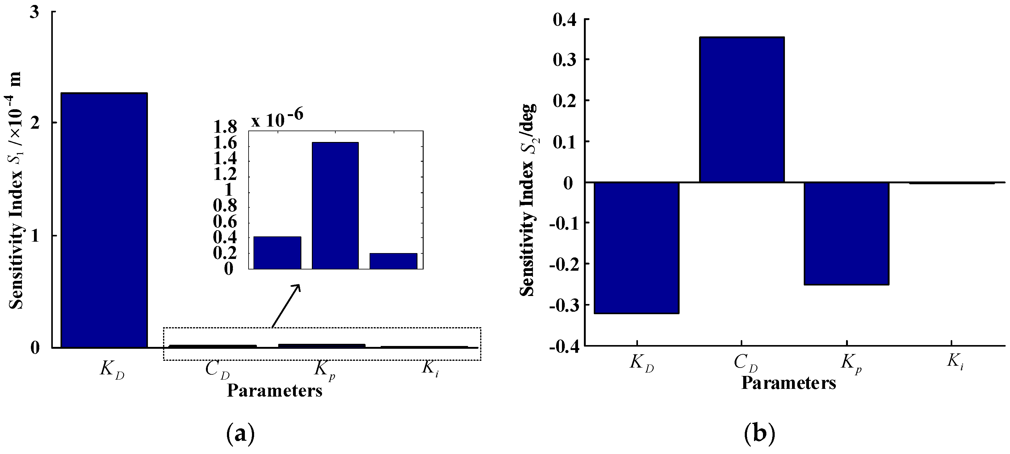
Figure 20.
Sensitivity histogram in the third working condition. (a) Sensitivity index ; (b) Sensitivity index .
Figure 20.
Sensitivity histogram in the third working condition. (a) Sensitivity index ; (b) Sensitivity index .
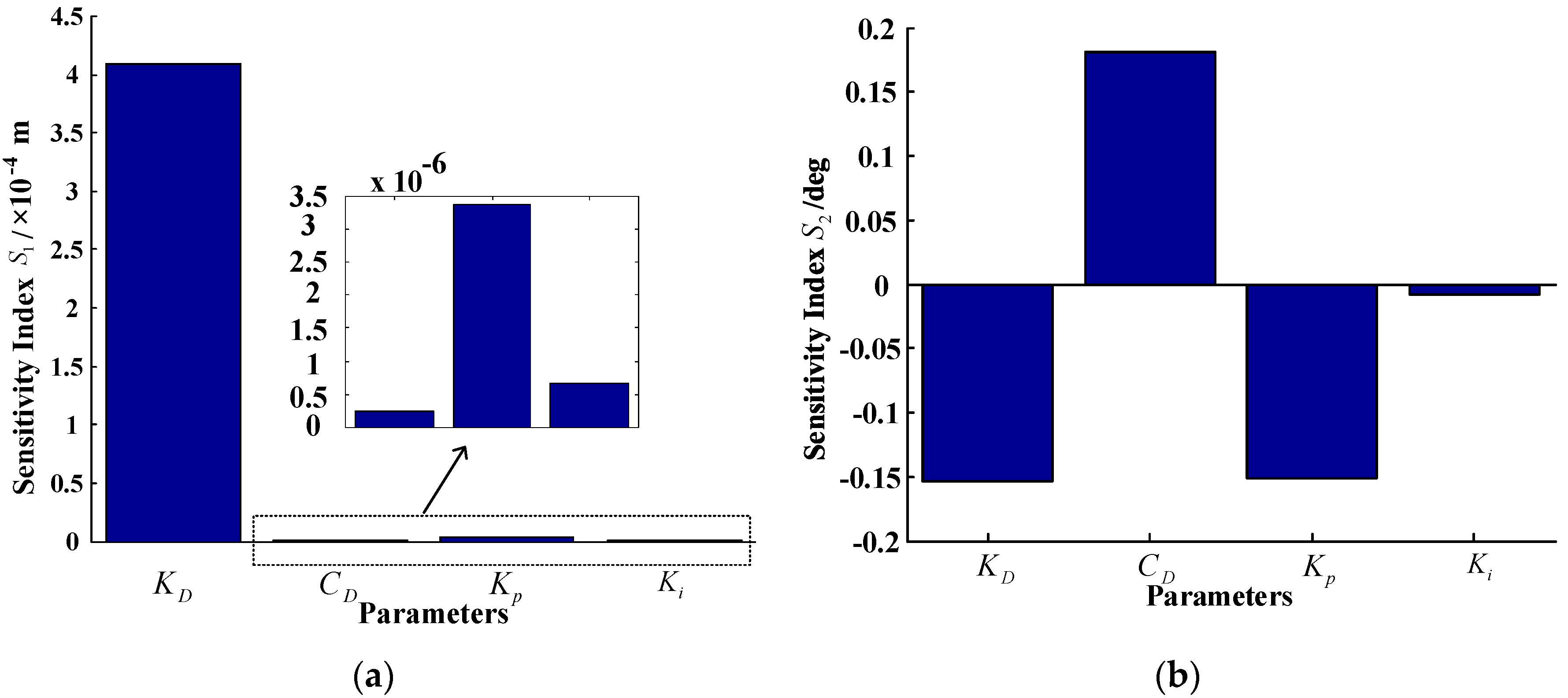
Figure 21.
Sensitivity histogram in the four working conditions. (a) Sensitivity index ; (b) Sensitivity index .
Figure 21.
Sensitivity histogram in the four working conditions. (a) Sensitivity index ; (b) Sensitivity index .
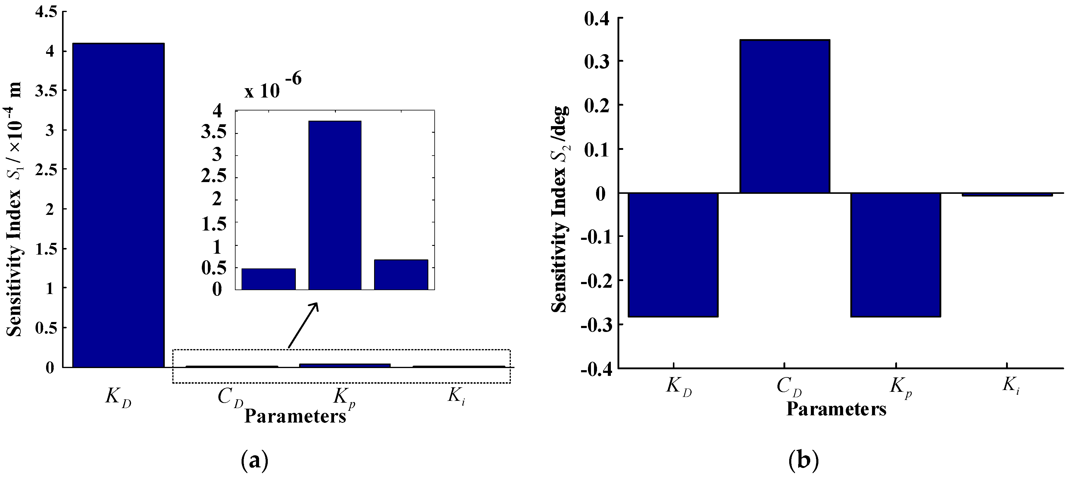
Figure 22.
Sensitivity index histograms of . (a) Sensitivity index ; (b) Sensitivity index .

Figure 23.
Sensitivity index histograms of . (a) Sensitivity index ; (b) Sensitivity index .

Figure 24.
Sensitivity index histograms of . (a) Sensitivity index ; (b) Sensitivity index .

Figure 25.
Sensitivity index histograms of . (a) Sensitivity index ; (b) Sensitivity index .

Table 1.
Parameters and initial values of the simulation model.
| Parameter | Initial Value |
|---|---|
| Gain of servo valve / | 0.0225 |
| Natural frequency of servo valve / | 628 |
| Damping ratio of servo valve | 0.77 |
| Effective piston area Ap/m2 | 3.368 × 10⁻⁴ |
| Volume of inlet chamber /m3 | 6.2 × 10⁻⁷ |
| Volume of outlet chamber /m3 | 8.6 × 10⁻⁷ |
| Piston stroke L/m | 0.05 |
| Initial position of piston L0/m | 0.025 |
| Supply pressure Ps/Pa | 1 × 10⁻⁷ |
| Tank pressure P0/Pa | 0.5 × 10⁶ |
| Gain of position sensor /() | 54.9 × 10⁻³ |
| Outer linkage coefficient of servo valve /(m3/(s·Pa)) | 0 |
| Inner linkage coefficient of servo valve /(m3/(s·Pa)) | 2.38 × 10⁻¹³ |
| Equivalent mass mt/kg | 1.1315 |
| Effective bulk modulus βe/Pa | 8 × 10⁸ |
| Conversion coefficient Kd | 1.248 × 10⁻⁴ |
| Load stiffness K/(N/m) | 0 |
| Viscous damping coefficient Bp/() | 54.9 × 10⁻³ |
| proportional gain | 30 |
| differential gain | 10 |
| Desired stiffness /() | 1 × 10⁶ |
| Desired damp /() | 5 × 10⁴ |
| Desired mass /kg | 0 |
Table 2.
Four working conditions researched in this paper.
| No. | Working Conditions | |
|---|---|---|
| Frequency (Hz) | Bias, Amplitude (N) | |
| 1 | 1 | 1500, 1000 |
| 2 | 2 | 1500, 1000 |
| 3 | 1 | 2500, 2000 |
| 4 | 2 | 2500, 2000 |
Table 3.
Mean values of performance indexes in different conditions.
| Performance Index | No. | ||||
|---|---|---|---|---|---|
| 1 | 2 | 3 | 4 | ||
| Amplitude reduction (mm) | Experimental | −0.05 | −0.09 | −0.06 | −0.11 |
| Simulation | −0.03 | −0.06 | −0.03 | −0.06 | |
| Phase angle delay (°) | Experimental | 7.8 | 6.7 | 8.9 | 9.4 |
| Simulation | 5.2 | 5.3 | 7.1 | 7.5 | |
Table 4.
Maximum and mean errors between experimental value and simulation value.
| Parameters | Max Error | Mean Error | Max Error | Mean Error |
|---|---|---|---|---|
| 19% | 12% | 20% | 16% | |
| 11% | 5% | 18% | 9% | |
| 31% | 16% | 15% | 10% | |
| 35% | 15% | 21% | 11% |
© 2017 by the authors. Licensee MDPI, Basel, Switzerland. This article is an open access article distributed under the terms and conditions of the Creative Commons Attribution (CC BY) license (http://creativecommons.org/licenses/by/4.0/).
Share and Cite
MDPI and ACS Style
Ba, K.; Yu, B.; Gao, Z.; Li, W.; Ma, G.; Kong, X. Parameters Sensitivity Analysis of Position-Based Impedance Control for Bionic Legged Robots’ HDU. Appl. Sci. 2017, 7, 1035. https://doi.org/10.3390/app7101035
AMA Style
Ba K, Yu B, Gao Z, Li W, Ma G, Kong X. Parameters Sensitivity Analysis of Position-Based Impedance Control for Bionic Legged Robots’ HDU. Applied Sciences. 2017; 7(10):1035. https://doi.org/10.3390/app7101035
Chicago/Turabian StyleBa, Kaixian, Bin Yu, Zhengjie Gao, Wenfeng Li, Guoliang Ma, and Xiangdong Kong. 2017. "Parameters Sensitivity Analysis of Position-Based Impedance Control for Bionic Legged Robots’ HDU" Applied Sciences 7, no. 10: 1035. https://doi.org/10.3390/app7101035
Note that from the first issue of 2016, this journal uses article numbers instead of page numbers. See further details here.