Obstacle Avoidance with Potential Field Applied to a Rendezvous Maneuver

1
Department of Mechanical and Aerospace Engineering, Politecnico di Torino, Corso Duca degli Abruzzi 24, 10129 Torino, Italy
2
National Council of Research, Institute of Electronics, Computer and Telecommunication Engineering (CNR–IEIIT), Corso Duca degli Abruzzi 24, 10129 Torino, Italy
*
Author to whom correspondence should be addressed.
Appl. Sci. 2017, 7(10), 1042; https://doi.org/10.3390/app7101042
Submission received: 31 July 2017
/
Revised: 26 September 2017
/
Accepted: 26 September 2017
/
Published: 12 October 2017
(This article belongs to the Section Mechanical Engineering)
Abstract
:This paper outlines a method based on the theory of artificial potential fields combined with sliding mode techniques for spacecraft maneuvers in the presence of obstacles. Guidance and control algorithms are validated with a six degree-of-freed (dof) omorbital simulator. The idea of this paper is to provide computationally efficient algorithms for real time applications, in which the combination of Artificial potential field (APF) and sliding mode control shows the ability of plan trajectories, even in the presence of external disturbances and model uncertainties. A reduced frequency of the proposed controllers and a pulse width modulation (PWM) of the thrusters are considered to verify the performance of the system. The computational performance of APF as a guidance algorithm is discussed and the algorithms are verified by simulations of a complete rendezvous maneuver. The proposed algorithm appears suitable for the autonomous, real-time control of complex maneuvers with a minimum on-board computational effort.
1. Introduction
Rendezvous maneuvers are a fundamental step for space exploration, and autonomous rendezvous and proximity operations have been expanded over the last decades. Since the beginning of the space era, orbital manned rendezvous and docking maneuvers have been studied and tested, in the Gemini program [1], with the purpose to dock two spacecraft to be able to reach the Moon, land on it, and safely return the crew on Earth in the Apollo program [2]. Cooperation between the United States and Russia made possible the rendezvous and docking of two space vehicles of completely different concepts, such as in the Apollo–Soyuz Test Project [3]. More recently, automated missions to bring supplies to the International Space Station (ISS) have been continuously flying, involving different type of spacecraft (ATV (Ariane Transfer Vehicle) [4], HTV (H-II Transfer Vehicle) [5], Progress [6], Cygnus [7], and more). Since these are unmanned spacecraft, an automated rendezvous mission has to be successfully completed. This brief introduction empathizes the importance of manned and unmanned rendezvous missions.
Recent studies concern the use of unmanned spacecraft in orbital servicing missions, such as the on-orbit refueling of telecommunication satellites, to extend their operational life (the operational life of many satellites is usually limited due to expired propellant, required for station-keeping) or space tugs [8,9,10]. In both cases, since such spacecraft are unmanned, a robust flight software must be developed. Even though the ground segment has the role of mission director in automated missions too, a number of unexpected events may appear, and have to be managed; namely, (i) unforeseen orbit crossing of small objects, such as moving of robotic arms in an ISS (International Space Station) scenario; (ii) delays or lack of communication with the control center; and (iii) environment disturbances and sensor noise. All the events described before have to be taken into account and the Guidance, Navigation and Control (GNC) software must be able to react properly. For this purpose, a robust and accurate simulation tool is very useful to develop and test GNC software.
The objective of the present work is the development of a six degree-of-freedom (dof) orbital simulator and the design and implementation of guidance and control algorithms, able to avoid obstacles. The approach proposed for the guidance algorithm is based on the theory of artificial potential fields with a paraboloid-based shape. For the control algorithms, for both position and attitude dynamics, sliding mode controllers (SMC) are proposed. The orbital simulator is written in C, as well as the GNC software. Communications between the simulation block and the on-board software block is allowed by a proper Transmission Control Protocol (TCP). Two separates algorithms are implemented: (i) one related to the simulator and (ii) one related to the GNC system, to design a flight software as close as possible to the “flyable” format and to formally separate the physical simulation and the software component, as required by EASA (European Aviation Safety Agency) standards [11]. A local connection is considered in which the six dof simulator is the server and the GNC system is the client. The simulator sent sensor data to the GNC system and the GNC sent the input data, related to the thruster switch on and the reaction wheels’ torque to the simulator. In this way, a two channel segment is considered, as for real space software, in which the space segment includes attitude and control systems and the ground segment has simulators and flight dynamics systems. Hardware constraints are also included.
The examined case is a rendezvous maneuver, in which an active vehicle (Chaser) orbits kilometers away from a passive vehicle (Target) and it has to reach and, eventually, dock it. Rendezvous and docking could be seen as a planned collision of two spacecraft, controlled considering the geometric location of the contact points on the two vehicles, and the linear velocities and angular rates at contact. Most of the literature assumes that the Chaser may access any region of the maneuver in the space. However, many scenarios involve operations near large space structures or, due to the increase of space debris, in proximity to obstacles [12]. Consequently, one of the essential requirements for automated rendezvous operations is the ability to maneuver in proximity to them, without collision. The motivation of this research is to safely reach the Target without collisions, designing an analytical and computationally efficient (real time) method.
For close range maneuvers, the guidance and control (GC) algorithms must be able to handle actuator constraints as well as dynamic and obstacle constraints. For this reason, the guidance algorithms for the complete rendezvous maneuver are based on the theory of artificial potential fields.
Artificial potential fields (APFs) have evolved in the past years for guiding the motion of mobile robots. The main idea of the artificial potential field theory is to construct a potential field with a gradient acting attractively toward the goal and repellently from obstacles. Different approaches using artificial potential fields are proposed in literature. An obstacle avoidance algorithm for a rendezvous maneuver is proposed in [13]. Two limitations of this approach are: (i) an “ad hoc” method for guidance is proposed and (ii) the control algorithm works at high frequency. Starting from this work in [14], a method for spacecraft maneuver with obstacles is proposed, but no control algorithms are considered and a simple dynamics is analyzed. In a similar way, real-time on-board execution of APF as guidance scheme is analyzed in [15]. More recently, interesting applications of APF as guidance algorithms are proposed in [16,17]. In [16], an adaptive artificial field for proximity operations is considered and the computational efficiency is proven in an experimental testbed. In [17], a near optimal hybrid guidance method using APF is proposed, combined with a sample based path planning method. In both cases, the APF algorithm is used as a GNC system and an “ad hoc” field is generated. Moreover, only a forced motion is considered. In our work, feedback control based on SMC theory is designed for tracking the gradient, generated by the APF algorithm. Our idea is to propose a method for an orbital spacecraft maneuver in which obstacles and external disturbances are considered. Moreover, the proposed algorithm is able to guarantee real time applications, considering the requirements of current space hardware (limitations of the sample frequency). In Feng et al. [18] an optimal sliding mode combined with an APF algorithm is considered. In this research, only proximity maneuver and orbital dynamics are analyzed, even if external disturbances are included.
In detail, the desired velocity and the desired attitude are defined by the APF algorithm to track the desired trajectory and avoid obstacles. This interpretation of the gradient was proposed in [19], in which a sliding mode control strategy for tracking the gradient due to a artificial potential field is described. In [20], the problem of controlling an autonomous wheeled vehicle with a SMC is proposed, including collision avoidance. The use of SMC in this context proves to be appropriate because of its robustness features. Usually, pseudo-sliding mode control, as in [21], based on continuous approximations, are proposed for mechanical systems. For spacecraft maneuver and, in particular, for position dynamics, a conventional first order SMC is the most suitable, due to the thrusters, for which the designed control signals are discontinuous. The advantage of the use of the artificial potential fields for this maneuver is twofold: (i) an autonomous way for the desired path is designed with low computational effort and (ii) an online update of the path is guaranteed, in particular in the presence of obstacles. The idea of this paper is to provide computationally efficient algorithms for real time applications in space. The novelties are related to the combination of APF and sliding mode controller (SMC) for a complete space maneuver, in which the SMC design is focused on a real application: (1) reduced frequency of the controller for fuel saving, (2) pulse width modulation of thrusters, and (3) actuator models are considered. For APF algorithms, even if the approach is well known, we propose a simple shape of the artificial field to have a reliable method (the same field for all the maneuver) and to avoid obstacles. In our case, external disturbances are also considered, to demonstrate the robustness of the proposed controller.
The paper is organized as follows. In Section 2, a detailed spacecraft model is analyzed, including actuator models, position and attitude dynamics, and external disturbances. The proposed guidance algorithms are described in Section 3; instead, the sliding mode control strategies are presented in Section 4. The simulation results are in Section 5. Conclusions are drawn in Section 6.
2. Orbital Simulator
The orbital simulator includes the six dof spacecraft dynamics, model of the actuation system (Reaction Control Thrusters (RCS) and reaction wheels (RWs)), models of sensors, and model of external disturbances. Actuators and sensors errors and nonlinearities are also taken into account.
The spacecraft dynamics includes both position dynamics and attitude dynamics. The orbital dynamics is based on propagation of equations of relative dynamics, usually known as Hill’s or Clohessy-Wiltshire equations. Attitude dynamics is formulated in the quaternion notation and it is propagated relative to the inertial Earth Centered Inertial reference frame (ECI).
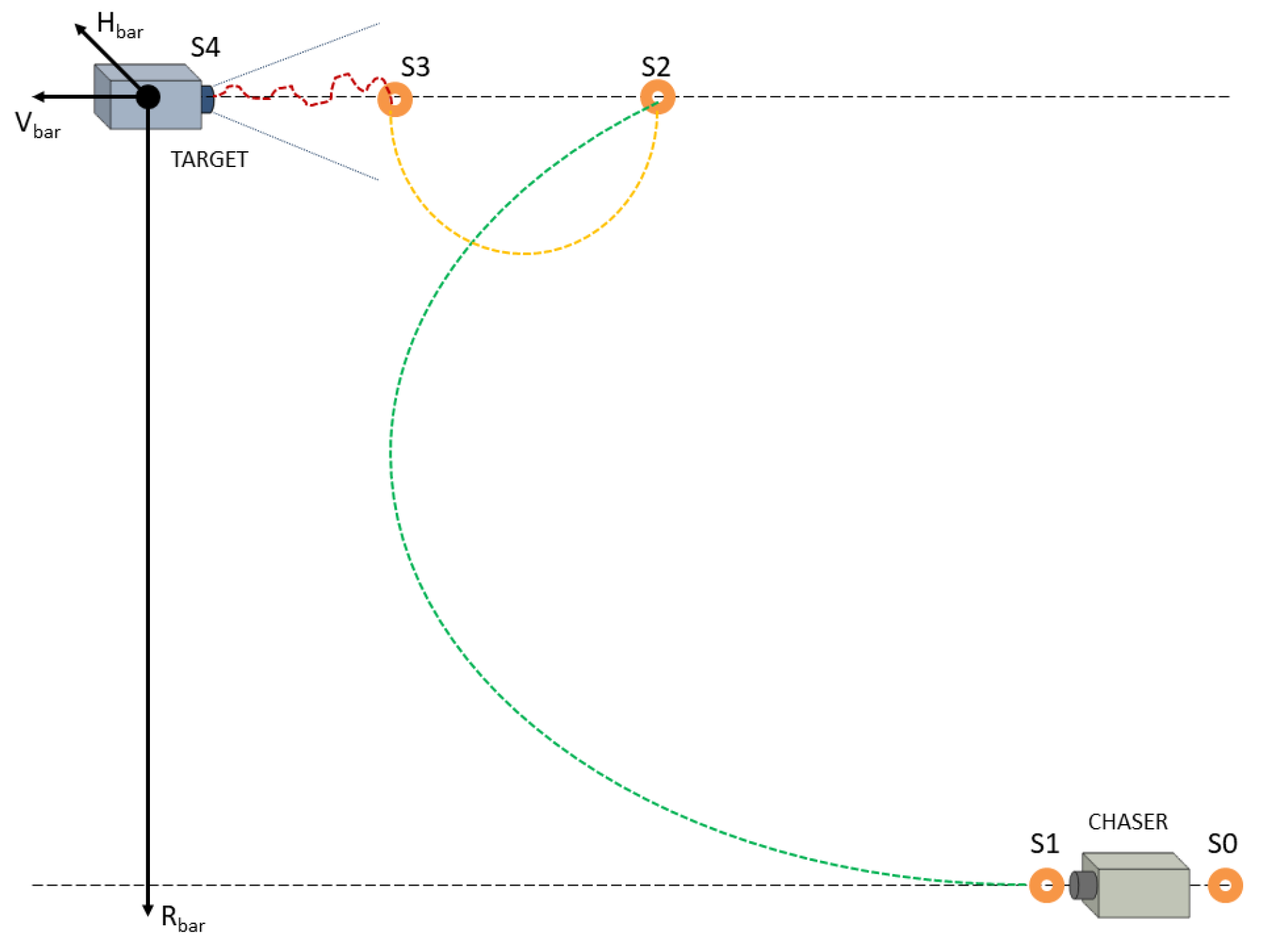
As briefly said in the introduction, the proposed case study is a complete rendezvous maneuver depicted in Figure 1. The Hill frame will be described later in the paper, and it will be better depicted in Figure 2. The maneuver starts at the waypoint S0, which is the initial condition for the simulation. This waypoint corresponds to a lower orbit with respect to the Target one and it is located at a sufficient distance from the Target in order to successfully complete the maneuver. The second part of the complete maneuver is for reaching the Target orbit and it starts at waypoint S1, the position of which depends on the difference in altitude between the two spacecraft. If the maneuver is an impulsive (or quasi-impulsive) one, the resultant trajectory corresponds to the ideal Hohmann transfer. The next maneuver (from waypoint S2 to waypoint S3) is necessary for getting closer to the Target. The distance of S3 from the Target is usually of the order of hundreds of meters, and it is strongly dependent on safety approach issues. Finally, waypoint S4 corresponds to the docking mechanism of the Target. The S3–S4 maneuver is a forced motion of the Chaser to get the Target, generally similar to a straight line approach. The simulation stops when the Chaser is few meters away from the Target. The docking of the spacecraft is not considered in the simulator, because a multibody dynamics is usually considered to clearly understand the loads of contact.
2.1. Spacecraft Position Dynamics
The complete description of the derivation of Hill’s equations from inertial equations is extensively described in [22], while in the following it is reported as the final formulation. Hill’s equations describe the relative motion between two objects orbiting in slightly different orbits. Hill’s equations are computed with respect to the origin of a Local-Vertical-Local-Horizontal (LVLH) reference frame (Figure 2), usually coincident with the center of mass of the Target. The reference object may also be taken as a virtual point as the origin of the LVLH frame orbiting the Earth, where the position dynamics of more spacecraft can be propagated with respect to it. Some assumptions have to be formulated.
- The orbit of the reference object must be circular. However, a modified formulation of Hill’s equations for non-circular orbits can be found in literature [23].
- The validity of the approximation of Hill’s equations is limited to few kilometers of distance along each axes. Introduction of curvilinear x and y coordinates may partially extend the validity of Hill’s equations, mitigating position error due to the curvature of the Earth. In this paper, curvilinear coordinates are not implemented.
, and are also named respectively , and . Hill’s equations for circular orbit
where , and are accelerations in the LVLH frame; , and are velocities with respect to the LVLH frame; x, y, and z are Hill positions; is the mass of the spacecraft; and is the orbital angular velocity of the reference LVLH frame. is the total force acting on the spacecraft and it includes both forces due to the thrusters system and external disturbances
where is the thruster force and is the external disturbances perturbation, both expressed in the LVLH frame. The main disturbance affecting Low Earth Orbits (LEO), in terms of magnitude, is the drag force due to the residual atmosphere. For this maneuver, since oblateness of the Earth affects orbital parameters of the reference object and the relative position dynamics is computed with respect to the Target, the J2 effect can be usually considered one order of magnitude smaller than the drag force. Hence, the force due to external disturbance can be reduced to a constant atmospheric drag and to a random force due to J2 effect. The drag force is designed as
where is the density of the atmosphere, V is the orbital velocity of the spacecraft, S is the frontal section, and is the drag coefficient of the spacecraft. The negative sign of is due to the drag force is opposing the motion along +V-bar.
Basically, the RCS model is defined in Body frame, hence, to obtain the thrust force in the LVLH frame, a rotation has to be applied
where is the thrust force expressed in body frame (related to the actuation system) and is the rotation matrix from body frame to LVLH frame.
The actuation system for position control exploits thrusters and the adopted thrusters can exert mono-directional actions, that is they can apply to the Chaser thrusts of given magnitude and along fixed directions, which depend on how and where the thrusters have been assembled in the system (their orientations and application points).
As will be detailed in the following, in each required control direction a pair of actuators are placed and exert their mono-directional thrusts. Moreover these thrusters coupled by direction are always switched on together by the controller. This precise choice of design for the actuation system guarantees a nominal zero moment due to the thrusters in the ideal case, when no thruster errors occur. Then the total number of thrusters of the Chaser is always even.
Each thruster is characterized by a fixed output and can be only be turned on/off without modulation of the provided thrust. This means that, the individual thruster can provide either the maximum amount of thrust when switched on or no force when switched off.
Further characteristics of each thruster are given by the time duration of the pulse width and the thruster zero time before turning on again . In fact, if the controller switches on the thruster at time , this actuator provides the maximum thrust for a time and then the same thruster cannot be turned on again for a time , as shown in Figure 3 and according to the following
where and are known and constant for each thruster. The constant can be computed and its inverse constitutes the maximum allowed frequency at which the thruster can be switched on.
In our case, RCS is composed by 12 thrusters , as depicted in Figure 4.
The magnitude of the thrust produced by each thruster is affected by bias and random errors, as well as the thrust direction, which is also affected by both type of errors. The magnitude of each thruster i can be expressed by
is the nominal thrust , is the bias thrust error and is the thrust noise; both of these contributions are different for each thruster. A similar formulation has been used to model the thrust direction
in which is the unit vector representing the thrust direction of the thruster affected by errors, is the unit vector representing the nominal thrust direction of the thruster, is the rotation matrix relative to the nominal direction of the thruster computed with bias angles and is the rotation matrix relative to the nominal direction of the thruster computed with random angles. At the end, the thrust provided by the thruster expressed in the body frame can be computed as
and is the force provided by the thruster. The total force provided by the RCS is
2.2. Spacecraft Attitude Dynamics
The attitude dynamics is propagated using the quaternion formulation. Angular velocity in the body frame can be obtained by:
where is the angular acceleration vector, is the inertia tensor, is the total torque acting on the spacecraft, is the angular velocity of the spacecraft, is the inertia of the reaction wheels system, and is the angular velocity of the reaction wheels system. The total torque acting on the spacecraft is the sum of different elements
where is the torque due to the RCS, is the torque due to external disturbances, and is the torque generated by the reaction wheels system. The torque generated by the thrusters system is obtained by
where is the position of the thruster relative to the center of mass and is defined by Equation (5). The external torque affecting the attitude dynamics of the spacecraft is mainly due to the gravity gradient torque. Other torque disturbances such as aerodynamic torque and torque due to the solar radiation have been neglected in the framework of this paper. The gravity gradient torque can beevaluated as
where is the Earth’s gravitational constant, r is the magnitude of position vector of the spacecraft relative to the center of Earth and is related to the third column of the rotation matrix . Kinematic equations in quaternion form can be expressed as
with is the vector of quaternions and is defined as
where is the skew-symmetric matrix
For the quaternions, the following notation can also be used (useful for the SMC controller definition)
where is the vector of quaternions and is the quaternion matrix, defined as
where is the quaternion scalar component, is the vector of the first three components of the vector q and is the skew-symmetric matrix
The attitude is propagated with respect to the Earth Centered Inertial (ECI) frame.
As previously introduced, three reaction wheels, driven by electric motors powered by the spacecraft electrical power supply, are considered for the attitude control and they are managed and controlled by the onboard attitude control computer. A reaction wheel actuator produces a moment MRW, causing its angular momentum to increase. For the representation of a realistic model, a first order filter and a saturation on the maximum–minimum torque assigned by the RWs are also included in the actuator model.
3. Guidance Algorithms
The rendezvous maneuver requires, in the presence of obstacles, to be performed completely autonomously with only sensors and on-board GC algorithms. Moreover, the GC algorithms must be able to simultaneously achieve a series of translational maneuvers in the presence of external disturbances and uncertainties. The potential field method can produce low impulsive fuel and can be implemented online with a low computational effort. At each time step, the artificial potential field algorithm generates the desired velocity and orientation required for reaching the Target. The desired vectors are generated considering the end of each maneuver as a minimum and the obstacle as a maximum and are not known a priori (no predetermined trajectory is considered).
A paraboloid artificial potential field is considered because it is a stabilizing function, and we impose that, as the Chaser approaches the goal, its speed decreases. Two different artificial potential fields are considered: (i) one is related to the position dynamics and (ii) the second is related to the attitude dynamics.
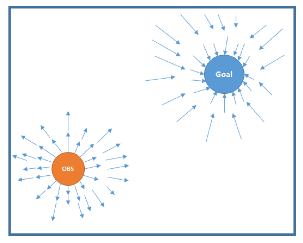
For the position dynamics, the artificial potential field is attractive to the goal and repulsive with respect to the obstacles. As in Figure 5. The attractive potential field is
where defines how fast the attractive gradient goes to the goal and is the error in position in which . The attractive force is due to the gradient of the artificial potential field. To assign the direction of the desired speed, a unit vector of the potential field is evaluated
thus the desired speed is evaluated as
where is the maximum speed to perform the maneuver, which is scalar and equal along the three axes.
To avoid the obstacles, a repulsive potential field is defined, one for each obstacle ( with number of obstacles)
where is the gain related to the repulsive field, is defined for hyperbolic field, , is the obstacle position, and is the safety radius. is the convex set of obstacles. The repulsive field is defined for each obstacles, which are assumed convex. As before, the repulsive force is
The radius for is the safety radius and it means that the Chaser “senses” the obstacle when it is m away from the obstacle. The applied artificial potential field is the sum of the attractive and repulsive part
and the total vector indicating the motion direction, opposite of the artificial potential field, is
with .
As explained before, the desired behavior is reached when the speed vector is collinear with . For this reason, the desired orientation with respect to the LVLH frame is obtained with the following definition of the orientation (Euler) angles
where the function arctan produces angles in the four quadrants of the Cartesian plane with . For example, the rotation matrix for the x rotation is
The total transformation matrix for the desired orientation is
From this matrix, we can easily evaluate the desired quaternion and the desired as in Equation (9).
In the last part of the maneuver (forced motion), we assume that the Chaser has to be aligned with the Target, so the desired attitude in terms of quaternions is , which means the body frame aligned with the ECI one.
4. Control Algorithms
As discussed in the introduction, we propose two different sliding mode controllers: (i) a first order SMC for spacecraft position tracking, guaranteeing tracking in terms of positions and speeds and (ii) a super-twisting SMC for the attitude control, including the quaternion dynamics.
4.1. Control System for the Position Dynamics
As deeply discussed in [24] and described for spacecraft maneuvers in [25], internal and external disturbances affecting the system due to the real implementation and to the external environment must be taken into account. Sliding mode methods provide controllers that are robust under large uncertainties. SMC can counteract uncertainties and disturbances, if the perturbations affecting the system are matched and bounded (first order SMC) or smooth matched disturbances with bounded gradient (second order SMC) [26,27].
For the position tracking, as already described in the introduction, a first order sliding mode is designed, motivated by the intrinsic nature of the thrusters, which cannot provide continuously modulated thrusts but can only be switched on and off.
The input vector (as in Equation (5)) is designed according to the following first order sliding mode control law
where , , being to reflect that two thrusters are switched on simultaneously, and represents the designed sliding output. In general, the control gain K in (18) must guarantee that the sliding motion on the desired sliding manifold is reached and maintained. The sliding output , which is the switching function in the controller (18), is
where and are the vectors of the desired speed and the desired positions, respectively. The vector of positions and speeds are measured at each time step from the Hill’s equations. The constant is chosen positive. The desired sliding surface is . The desired conditions are defined with the artificial potential fields, as described in the previous section.
4.2. Control System for the Attitude Dynamics
Concerning the attitude stabilization, it should be remarked that it represents a problem of particular importance for spacecraft, since it is fundamental for enforcing precision and also for guidance, as short propulsive maneuvers must be executed with extremely accurate alignment [28]. A second order sliding mode (two-sliding mode) algorithm, known as super-twisting (STW) [27], is considered for the attitude tracking. The STW algorithm designs a continuous control law, which steers to zero in finite time both the sliding output and its first time derivative. This continuous controller is suitable for the actuation system related to the attitude dynamics (reaction wheels). Moreover, since the STW algorithm contains a term that is obtained as the integral of a discontinuous component, the chattering is strongly attenuated.
5. Numerical Simulations
As already mentioned in the introduction, the idea of this paper is to combine APF and SMC controllers and to replan online the trajectories in presence of obstacles, verifying the computational effort required for these algorithms. The simulation model is tested for a generic Chaser–Target combination involved in sequential flight phases, as in Figure 1. The Chaser is considered in stable initial conditions along an orbit of height km, and the Target center of mass is located at the origin of the LVLH reference frame, and it is 16 km far from the Chaser. A cubic-shape Chaser (1.2 m) is considered with an initial mass of 600 kg, as in Table 1. The location of the four waypoints is summarized in Table 2.
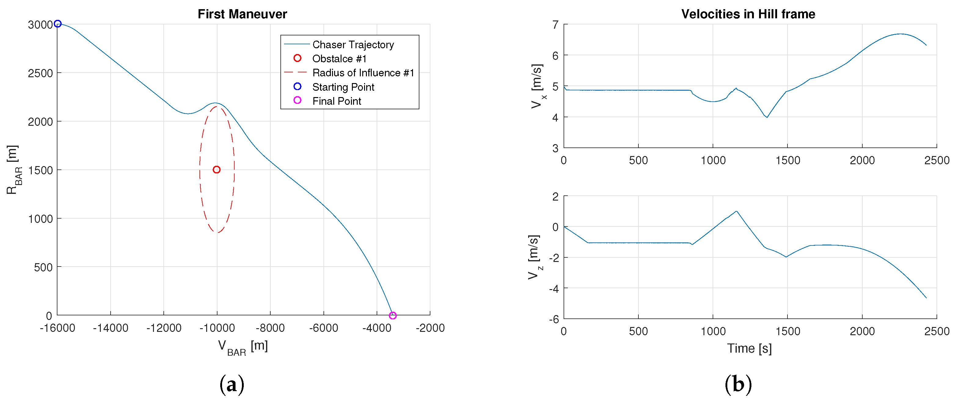
The proposed approach is compared with the combination of the APF and Linear Quadratic Regulator (LQR) controller for the first phase of the maneuver. An LQR controller is designed for the position dynamics, instead a constant attitude (i.e., the Body and LVLH frame aligned) is considered for this combination. External disturbances and sensor noise are included for both cases. The maximum value of the thruster errors (bias and random values) is equal to the 10% of the maximum thrust. The gain matrix of the LQR controller is set considering an ideal impulsive Hohmann maneuver. For this reason, the end point of the maneuver is about −8 km, as in Figure 6. A PWM behavior is not evaluated for the LQR controller, so a continuous thrust is assigned. If an obstacle is included in the evaluation of the first maneuver, we can observe that, even if the safety radius is 1000 m, the position dynamics is deviated only when the Chaser is inside the safety zone, with a speed on the X axis that is about 6 m/s. A zero altitude is reached as desired.
The ideal maneuver profile described in both Figure 1 and Table 2 is affected by three obstacles that the Chaser shall safely avoid, thanks to the artificial potential field algorithm definition. Obstacles are defined considering a center of application and a safety radius, as described in Section 3. As first approximation, all the obstacles are considered in a fixed known position. Their location is summarized in Table 3 and different safety radii are considered.
The simulated maneuver is depicted in Figure 1. The resulting maneuver is substantially different from the nominal one (Figure 1) because the Chaser deviates its path from the ideal one to avoid obstacles along the nominal path. The ellipsoidal shape of the radius of influence of the obstacles is due to the axis scaling.
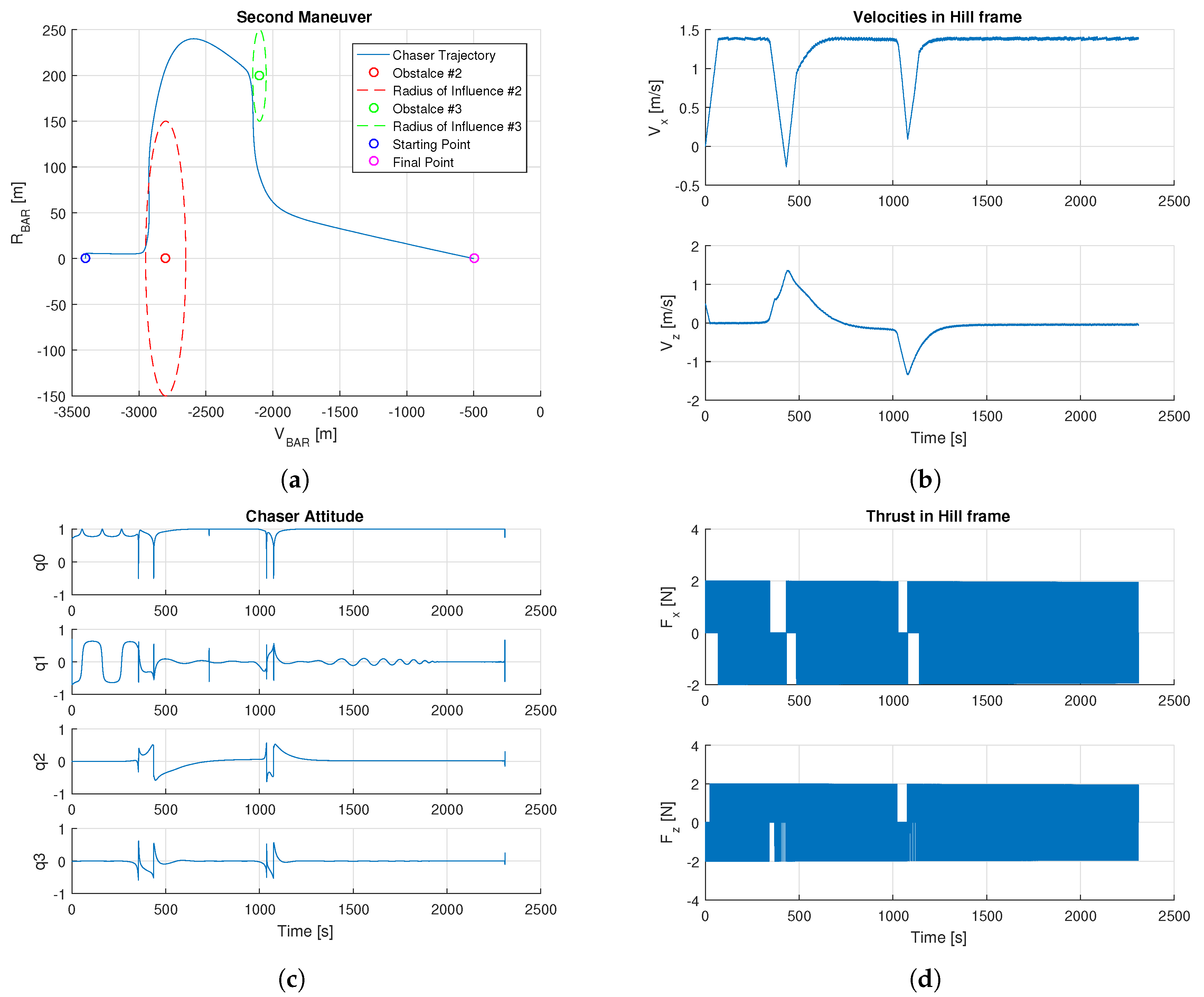
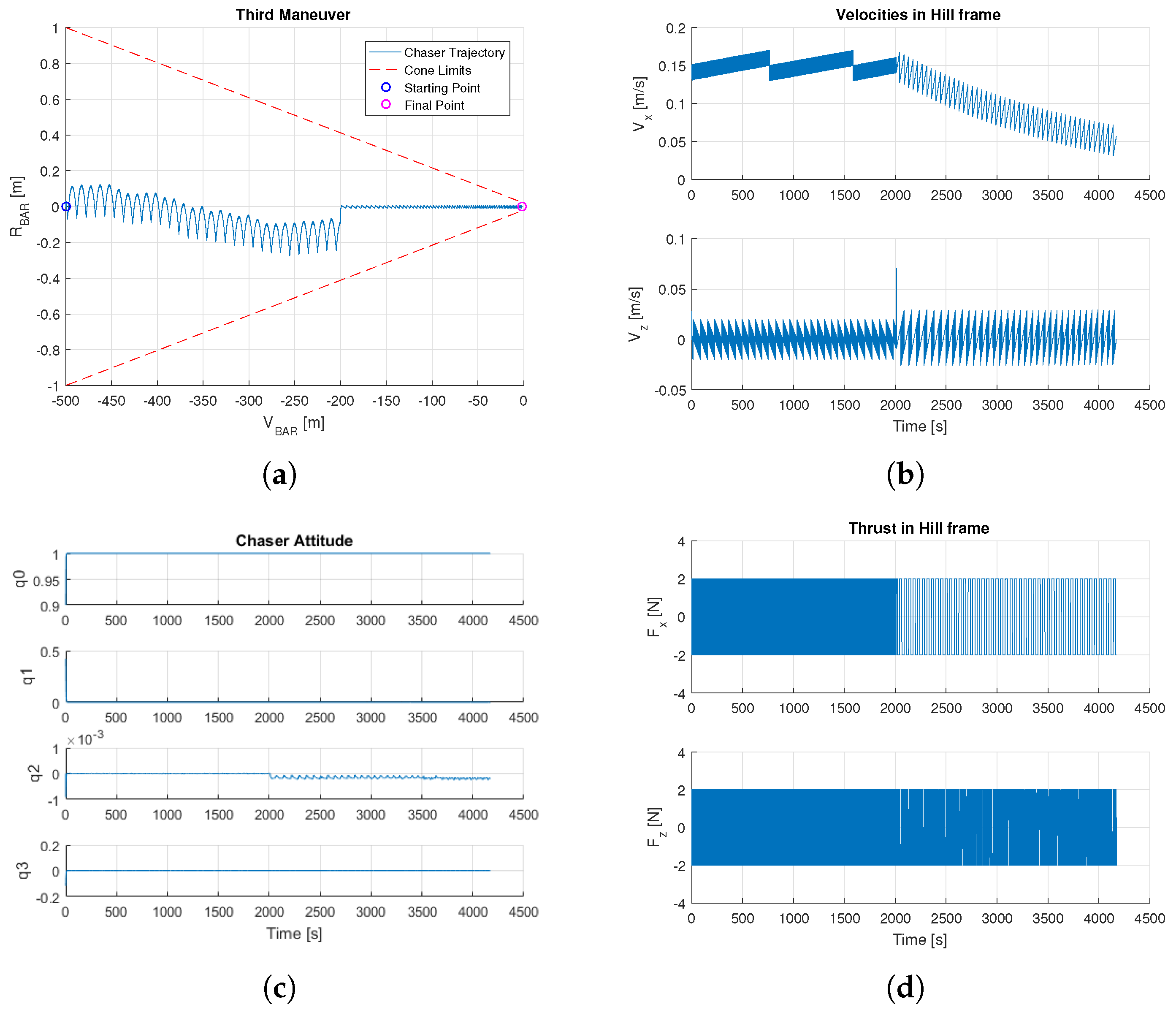
The three phases of the maneuver are separately discussed. In the first part of the maneuver, a single obstacle is considered. A PWM behavior can be observed in the thrust variations and the sample time of the thrusters switching on is set equal to 1 s, to reduce the fuel consumption due to the combination of APF and SMC. Usually, the SMC frequency is very high (close to infinity) to obtain good performance, but, in our case, we reduce the frequency of SMC to take into account the hardware limitations and to reduce the fuel consumption. Concerning Figure 7c, the relative quaternion has peaks and discontinuities because the APF algorithm changes the desired attitude, in accordance to Equation (17), when the Chaser is close to the obstacle. In the second phase, Figure 8, two obstacles with different safety radii are included, to evaluate the performance of the APF algorithm. In that case, we can observe that the Chaser is moving few meters inside the area of the first obstacle of the maneuver delimited by the safety radius. This is due to the value of the repulsive gain of Equation (12) related to the obstacle. Even if the maneuver is executed in safely manner, a more suitable tuning of this gain is required to completely satisfy the requirements. If an adaptive gain is chosen, better performance could be observed in proximity of obstacles. In the final approach maneuver, Figure 9, the desired positions are defined in accordance to the cone geometry where the maximum amplitude of the cone is m at the beginning of the maneuver and the final is m. No obstacles are considered because the Chaser is too close to the Target. Different switching frequencies are chosen to reduce the fuel consumption. All the constraints are satisfied, even if a reduced frequency is considered in the first part of the forced motion.
6. Conclusions
In this paper a guidance algorithm based on the theory of artificial potential fields is proposed. This method is combined with sliding mode techniques for both the control of position and attitude for real time space applications. A complete rendezvous maneuver is analyzed, in presence of obstacles. A “quasi-flyable” six dof simulator is considered for the validation of the proposed algorithms, in which both the ground and space segment are implemented in C language. Good results are obtained and the efficiency of the algorithms, also in terms of the computational effort, is proven. In future works, adaptive attractive and repulsive gains of the potential fields will be considered to satisfy the strict requirements of the maneuver and of the required safety. Moreover, dynamic obstacles will be considered. Experimental tests will be performed to prove the efficiency of the combination APF and SMC algorithms.
Author Contributions
Nicoletta Bloise, Elisa Capello, Matteo Dentis and Elisabetta Punta are equal to the contributions.
Conflicts of Interest
The authors declare no conflicts of interest.
References
- Hacker, B.C. On the Shoulders of Titans: A History of Project Gemini; NASA Technical Report; National Aeronautics and Space Administration: Washington, DC, USA, 1977.
- Young, K.A.; Alexander, J.D. Apollo Lunar Rendezvous; American Institute of Aeronautics and Astronautics: Reston, VA, USA, 1970. [Google Scholar]
- Ezell, E.C.; Ezell, L.N. The Partnership: A NASA History of the Apollo-Soyuz Test Project; Courier Corporation: North Chelmsford, MA, USA, 2013. [Google Scholar]
- Fabrega, J.; Frezet, M.; Gonnaud, J.-L. ATV GNC during rendezvous. Spacecr. Guid. Navig. Control Syst. 1997, 381, 85–93. [Google Scholar]
- Ueda, S.; Kasai, T.; Uematsu, H. HTV rendezvous technique and GNC design evaluation based on 1st flight on-orbit operation result. In Proceedings of the AIAA/AAS Astrodynamics Specialist Conference, Toronto, ON, Canada, 2–5 August 2010. [Google Scholar]
- Hall, R.; Shayler, D. Soyuz: A Universal Spacecraft; Springer Science & Business Media: Berlin, Germany, 2003. [Google Scholar]
- Miotto, P.; Draper Laboratory. Designing and Validating Proximity Operations Rendezvous and Approach Trajectories for the CygnusMission. In Proceedings of the AIAA/AAS GNC Conference, Toronto, ON, Canada, 2–5 August 2010; AIAA Paper. Volume 8446. [Google Scholar]
- Cresto Aleina, S.; Viola, N.; Stesina, F.; Viscio, M.A.; Ferraris, S. Reusable space tug concept and mission. In Proceedings of the International Astronautical Congress, Jerusalem, Israel, 12 October 2015; International Astronautical Federation (IAF): Paris, France, 2015; Volume 11. [Google Scholar]
- Wingo, D.R. Orbital recovery’s responsive commercial space tug for life extension missions. In Proceedings of the AIAA 2nd Responsive Space Conference, Los Angeles, CA, USA, 28–30 September 2004. [Google Scholar]
- Aslanov, V.; Yudintsev, V. Dynamics of large space debris removal using tethered space tug. Acta Astronaut. 2003, 91, 149–156. [Google Scholar] [CrossRef]
- Jones, M.; Gomez, E.; Mantineo, A.; Mortensen, U.K. Introducing ECSS Software-Engineering Standards within ESA; EASA Bulletin; European Aviation Safety Agency: Cologne, Germany, 2002. [Google Scholar]
- Frame, R., II. History of space shuttle rendezvous and proximity operations. J. Spacecr. Rocket. 2006, 43, 944–959. [Google Scholar]
- Tatsch, A.R.; Fitz-Coy, N. Dynamic Artificial Potential Function Guidance for Autonomous on-Orbit Servicing. In Proceedings of the 6th International ESA Conference on Guidance, Navigation and Control Systems, Loutraki, Greece, 17–20 October 2005. [Google Scholar]
- Martinson, N. Obstacle avoidance guidance and control algorithm for spacecraft maneuvers. In Proceedings of the AIAA Guidance, Navigation, and Control Conference, Chicago, IL, USA, 10–13 August 2009. [Google Scholar]
- Lopez, I.; McInnes, C.R. Autonomous rendezvous using artificial potential function guidance. J. Guid. Control Dyn. 1995, 18, 237–241. [Google Scholar] [CrossRef]
- Zappulla, R., II; Park, H.; Virgili-Llop, J.; Romano, M. Experiments on Autonomous Spacecraft Rendezvous and Docking Using an Adaptive Artificial Potential Field Approach. In Proceedings of the 26th AAS/AIAA Space Flight Mechanics Meeting, Napa, CA, USA, 14–18 February 2016. [Google Scholar]
- Zappulla, R., II; Virgili-Llop, J.; Romano, M. Near-optimal real-time spacecraft guidance and control using harmonic potential functions and a modified RRT. In Proceedings of the 27th AAS/AIAA Spaceflight Mechanics Meeting, San Antonio, TX, USA, 6–9 February 2017. [Google Scholar]
- Feng, L.; Ni, Q.; Bai, Y.; Chen, Z.; Zhao, Y. Optimal sliding Mode Control for Spacecraft Rendezvous with Collision Avoidance. In Proceedings of the IEEE Congress on Evolutionary Computation, Vancouver, BC, Canada, 25–29 July 2016; pp. 2661–2668. [Google Scholar]
- Guldner, J.; Utkin, V.I. Sliding mode control for gradient tracking and robot navigation using artificial potential fields. IEEE Trans. Robot. Autom. 1995, 11, 247–254. [Google Scholar] [CrossRef]
- Ferrara, A.; Rubagotti, M. Second-order sliding-mode control of a mobile robot based on a harmonic potential field. IET Control Theory Appl. 2008, 2, 807–818. [Google Scholar] [CrossRef]
- Edwards, C.; Spurgeon, K.S. Sliding Mode Control: Theory and Applications; Taylor and Francis: London, UK, 1998. [Google Scholar]
- Fehse, W. Automated Rendezvous and Docking of Spacecraft; Cambridge University Press: New York, NY, USA, 2003. [Google Scholar]
- Yamanaka, K.; Ankersen, F. New state transition matrix for relative motion on an arbitrary elliptical orbit. J. Guid. Control Dyn. 2002, 25, 60–66. [Google Scholar] [CrossRef]
- Utkin, V.I. Sliding Modes in Optimization and Control Problems; Springer: New York, NY, USA, 1992. [Google Scholar]
- Capello, E.; Dabbene, F.; Guglieri, G.; Punta, E.; Tempo, R. Sliding Mode Control Strategies for Rendezvous and Docking Maneuvers. J. Guid. Control Dyn. 2017, 40, 1481–1487. [Google Scholar] [CrossRef]
- Bartolini, G.; Ferrara, A.; Usai, E. Chattering Avoidance by Second-order Sliding Mode Control. IEEE Trans. Autom. Control 1998, 43, 241–246. [Google Scholar] [CrossRef]
- Levant, A. Sliding Order and Sliding Accuracy in Sliding Mode Control. Int. J. Control 1993, 58, 1247–1263. [Google Scholar] [CrossRef]
- Hughes, P.C. Spacecraft Attitude Dynamics; Dover Publications: London, UK, 2004. [Google Scholar]
Figure 1.
Complete rendezvous and docking maneuver in Hill frame.

Figure 2.
LVLH (Local-Vertical-Local-Horizontal) frame definition.
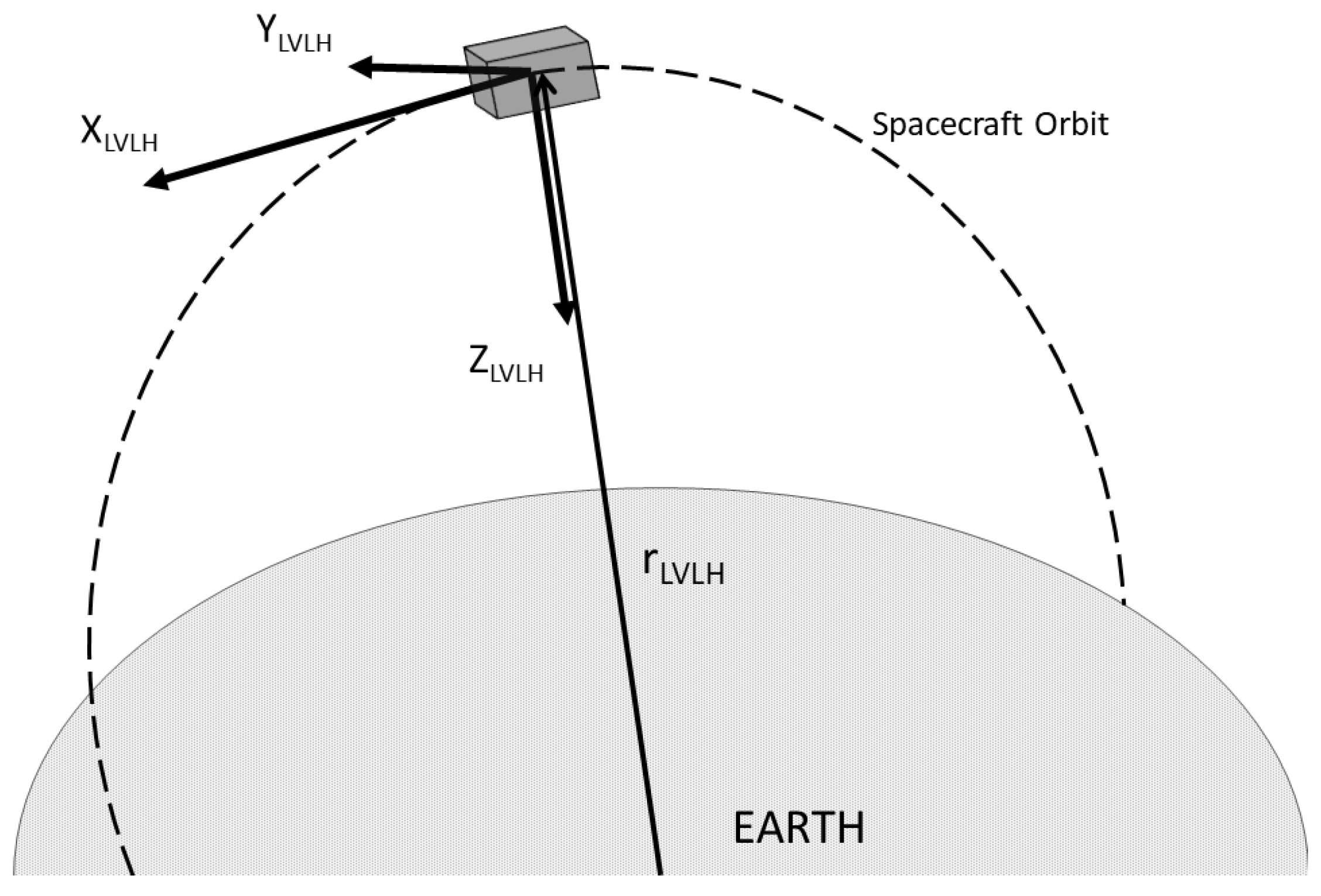
Figure 3.
Thrust provided by the thruster switched on at time .
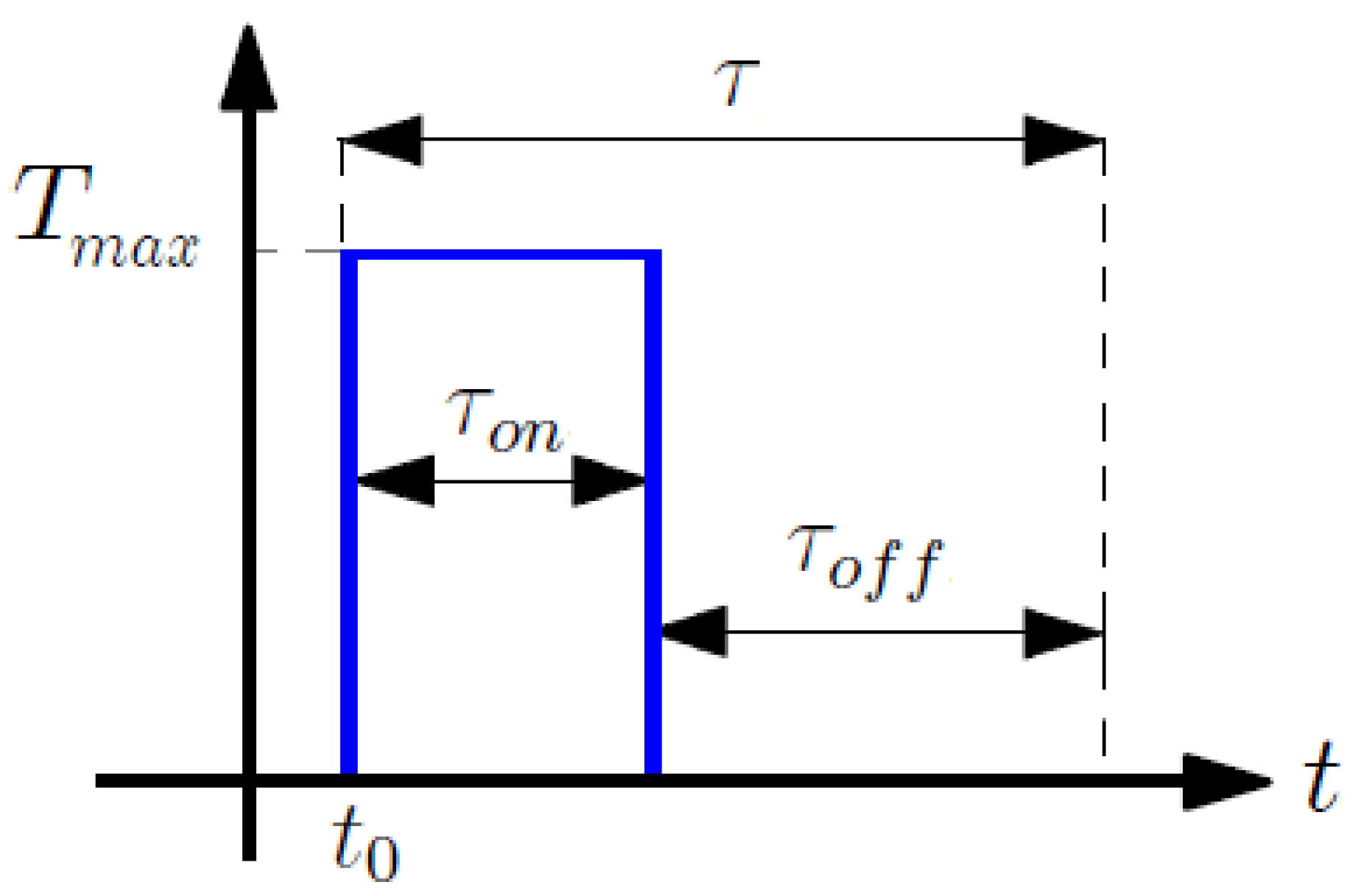
Figure 4.
RCS (Reaction Control Thrusters) configuration and body frame definition. CoG: Center of Gravity.
Figure 4.
RCS (Reaction Control Thrusters) configuration and body frame definition. CoG: Center of Gravity.
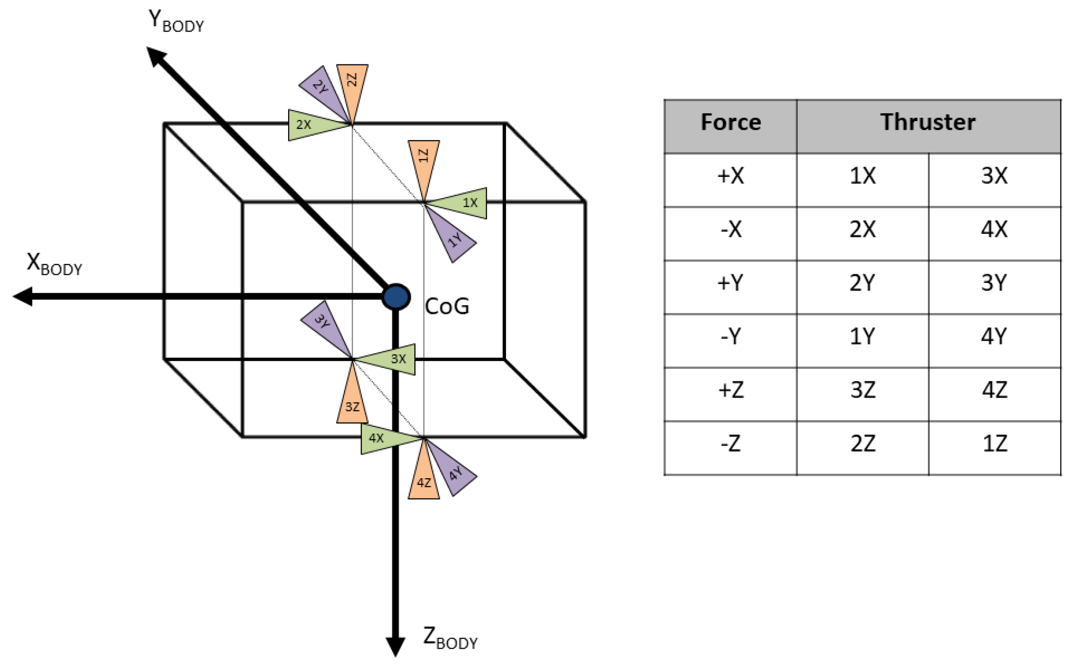
Figure 5.
Attractive and repulsive potential field.

Figure 6.
First maneuver highlights for the LQR (Linear Quadratic Regulator) controller. (a) First Maneuver: plane. The red circle represents the obstacle (dotted line = safety radius, red circle = obstacle center). (b) Relative velocity.
Figure 6.
First maneuver highlights for the LQR (Linear Quadratic Regulator) controller. (a) First Maneuver: plane. The red circle represents the obstacle (dotted line = safety radius, red circle = obstacle center). (b) Relative velocity.
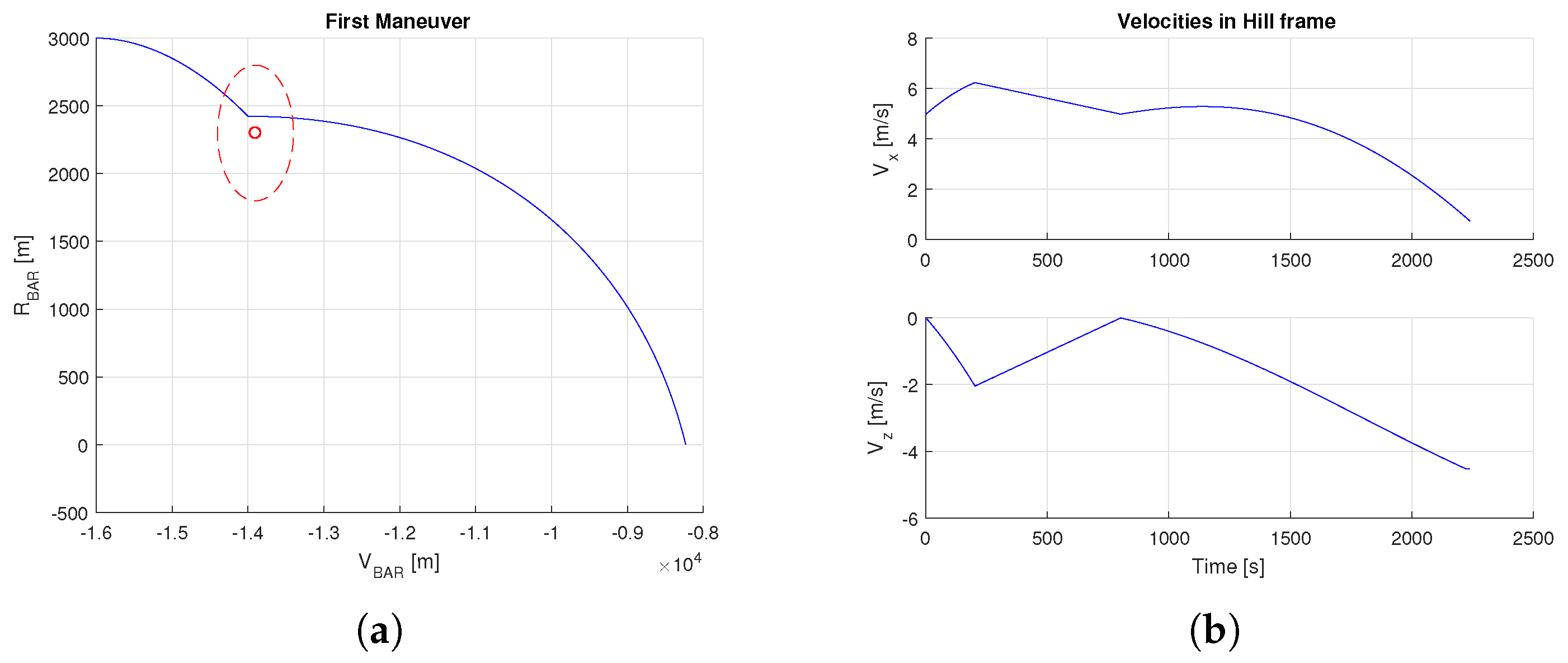
Figure 7.
First maneuver highlights for the SMC controller (sliding mode controllers). (a) First Maneuver: plane. (b) Relative velocity. (c) Relative quaternion. (d) Thrust profile.
Figure 7.
First maneuver highlights for the SMC controller (sliding mode controllers). (a) First Maneuver: plane. (b) Relative velocity. (c) Relative quaternion. (d) Thrust profile.

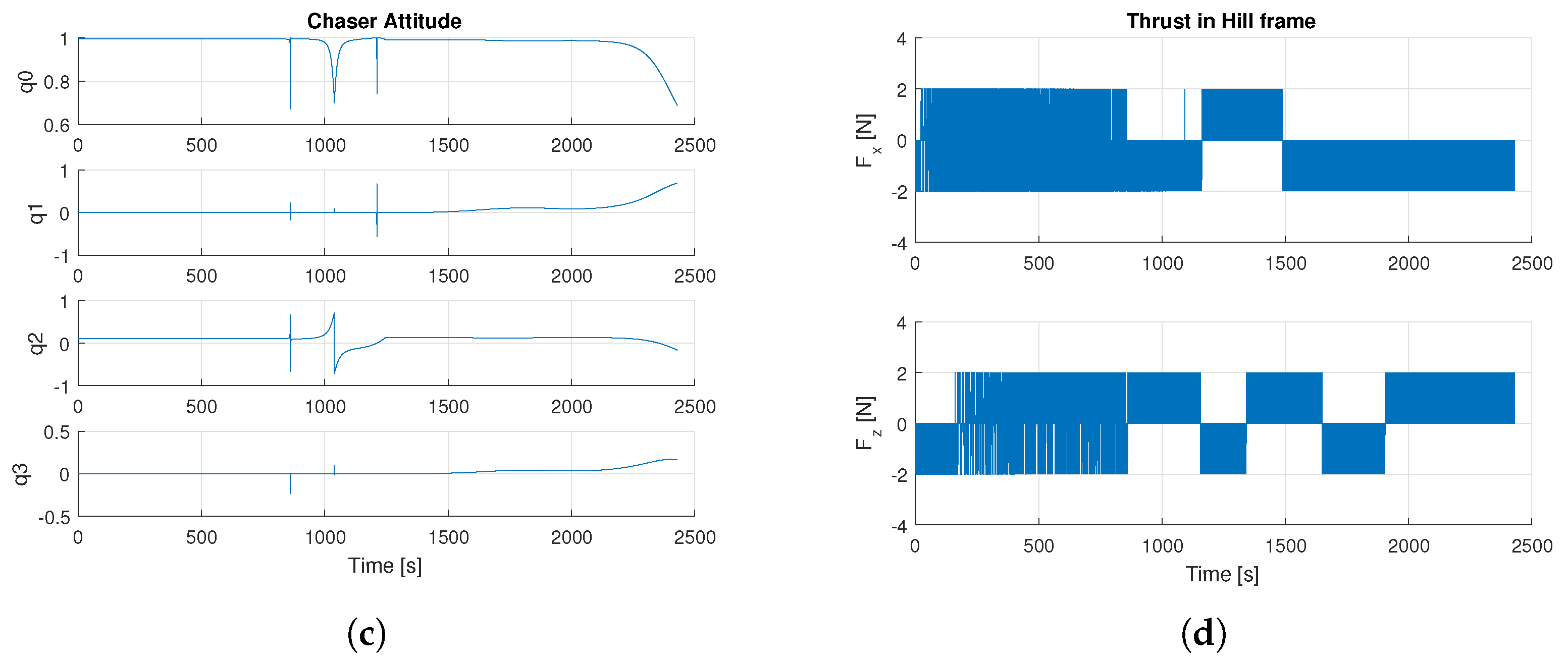
Figure 8.
Second maneuver highlights for the SMC controller. (a) Second Maneuver: plane. (b) Relative velocity. (c) Relative quaternion. (d) Thrust profile.
Figure 8.
Second maneuver highlights for the SMC controller. (a) Second Maneuver: plane. (b) Relative velocity. (c) Relative quaternion. (d) Thrust profile.

Figure 9.
Third maneuver highlights for the SMC controller. (a) Third Maneuver: plane. (b) Relative velocity. (c) Relative quaternion. (d) Thrust profile.
Figure 9.
Third maneuver highlights for the SMC controller. (a) Third Maneuver: plane. (b) Relative velocity. (c) Relative quaternion. (d) Thrust profile.


Table 1.
Chaser and Thruster characteristics. RW: reaction wheel.
| Parameter | Symbol | Unit |
|---|---|---|
| Initial mass | 600 kg | |
| Initial inertia tensor | kgm2 | |
| Zero shoot time of thrusters | 0.02 s | |
| Maximum thrust | 1 N | |
| Specific impulse of thrusters | 220 s | |
| RW Maximum torque | 1 Nm | |
| RW Inertial tensor | 0.1 kgm2 |
Table 2.
Waypoint LVLH position.
| Waypoint | Description | Position (m) |
|---|---|---|
| S0 | Initial simulation waypoint | [−16,100, 0, 3000] |
| S1 | Initial waypoint for Hohmann | [−16,000, 0, 3000] |
| S2 | Terminal waypoint for Hohmann/Initial waypoint for Radial Boost | [−3000, 0, 0] |
| S3 | Terminal waypoint for Radial Boost/Initial waypoint for Straight Line | [−500, 0, 0] |
| S4 | Terminal position |
Table 3.
Obstacles LVLH position.
| Obstacle Id. | Radius (m) | Position (m) |
|---|---|---|
| OBS #1 | 650 | [−10,000, 0, 1500] |
| OBS #2 | 150 | [−2800, 0, 0] |
| OBS #3 | 50 | [−2100, 0, 200] |
© 2017 by the authors. Licensee MDPI, Basel, Switzerland. This article is an open access article distributed under the terms and conditions of the Creative Commons Attribution (CC BY) license (http://creativecommons.org/licenses/by/4.0/).
Share and Cite
MDPI and ACS Style
Bloise, N.; Capello, E.; Dentis, M.; Punta, E. Obstacle Avoidance with Potential Field Applied to a Rendezvous Maneuver. Appl. Sci. 2017, 7, 1042. https://doi.org/10.3390/app7101042
AMA Style
Bloise N, Capello E, Dentis M, Punta E. Obstacle Avoidance with Potential Field Applied to a Rendezvous Maneuver. Applied Sciences. 2017; 7(10):1042. https://doi.org/10.3390/app7101042
Chicago/Turabian StyleBloise, Nicoletta, Elisa Capello, Matteo Dentis, and Elisabetta Punta. 2017. "Obstacle Avoidance with Potential Field Applied to a Rendezvous Maneuver" Applied Sciences 7, no. 10: 1042. https://doi.org/10.3390/app7101042
Note that from the first issue of 2016, this journal uses article numbers instead of page numbers. See further details here.