1. Introduction
Since forests are important for human life, forest inventories have been investigated for various purposes for centuries. In Europe, the first inventories were carried out in the 14th and 15th century for the purpose of intensive mine development. Since the 1910s, national forest inventories have been carried out in Norway, Sweden, and Finland, with an emphasis on timber production [
1]. However, the demands of society have changed rapidly over recent decades. In this context, the principles for the conservation and sustainable management of forests have been newly added by the United Nations General Assembly [
2]. This was in response to an increasing interest in non-timber aspects of forest structure and the demand for assessing these aspects [
3]. In the Republic of Korea, in the 1970s, when the forest inventory was first investigated, it was aimed at reforestation and forest statistics. The purpose of the forest inventory has changed as the value of forest resources and impacts on the environment have evolved. Currently, forest inventories are developed to provide information that is useful to achieve the following goals: to maintain a healthy forest ecosystem, to preserve and protect the global environment and to promote sustainable development [
4,
5,
6].
The vertical structure of a forest, which generally has four layers, is one of several elements representing forest vitality. In temperate zones, the forests are divided into layers of canopy, understory, shrub, and grass. The ability of the lower vegetation layer to grow under the canopy layer is determined by the condition of the soil, the species of vegetation, and the quantity of sunlight received by the lower vegetation layer due to the opening and closing rate of the crown [
7,
8,
9].
In the case of artificial forests, they are usually single- or double-layered forests, as they are planned and managed for the purposes of wood production and agriculture. Natural forests however, have formed from a variety of vegetation communities through natural succession over lengthy periods of time, and have multiple layers. From an ecological point of view, natural forests with multiple-layers are highly resistant to pests, diseases, and environmental stress, and have high quality ecosystem services, such as providing habitats for wildlife. This is not the case with single-layered forests [
10,
11,
12,
13,
14]. Therefore, vertical structure is a useful measure to evaluate the environmental aspects of a forest.
Typically, forest inventories have been investigated through terrestrial surveys. The Korea Forest Service currently uses aerial orthophotos to survey forests, but it is very difficult to understand forest structure because orthophotos only image the forest canopy. Thus, a field survey is required to understand the stratification of a forest. In Korea, more than 70% of the country is made up of mountainous areas, and a nationwide field survey would be very time- and cost-consuming. Since remote sensing data is advantageous for extensive regional studies [
15], we attempt to develop a method of effective forest inventory using remotely sensed data. Such a method could reduce the time and cost of a forest inventory.
Multi-layered mature forests normally have a rough texture in remotely-sensed images, while single-layered young forests have a smoother texture [
16,
17,
18]. Therefore, the structure of a forest can be estimated through the reflectance differences among the communities. The arrangement of the crown layer (canopy layer) in single-layered artificial forests can be considered consistent, but in natural forests it is inconsistent [
17,
18]. Since tree height is closely related to forest vertical structure, lidar data used for tree height measurements can be used to classify a forest’s vertical structure [
7,
19,
20,
21,
22,
23,
24]. Lidar is an abbreviation for light detection and ranging, and is a device that measures the distance of a target using laser light. The characteristics of remotely-sensed images and lidar data could enable us to classify the vertical structure of a forest.
The objective of this study is to classify forest vertical structure from aerial orthophotos and lidar data using an artificial neural network (ANN) approach. A total of five input layers are generated including: a median-filtered index map, a non-local (NL) means filtered index map, and reflectance texture map generated from the aerial orthophotos, and height difference and height texture maps generated from the lidar data. Since it is difficult to determine the presence of a grass layer in aerial images, it is omitted from our study and the forest vertical structure is classified into three groups for the ANN approach. The groups include: (i) single-layered forest that has only the canopy layer; (ii) double-layered forest that possesses the canopy layer and an understory or shrub layer; and (iii) triple-layered forest that is composed of the canopy, understory, and shrub layers. The red-green-blue (RGB) aerial orthophoto is used to obtain optical image information. The digital surface model (DSM) and digital terrain model (DTM) are extracted from the lidar point cloud. The height information is extracted by subtracting the DTM height from the DSM height. The accuracy of the classification is validated using field survey measurements.
2. Study Area and Dataset
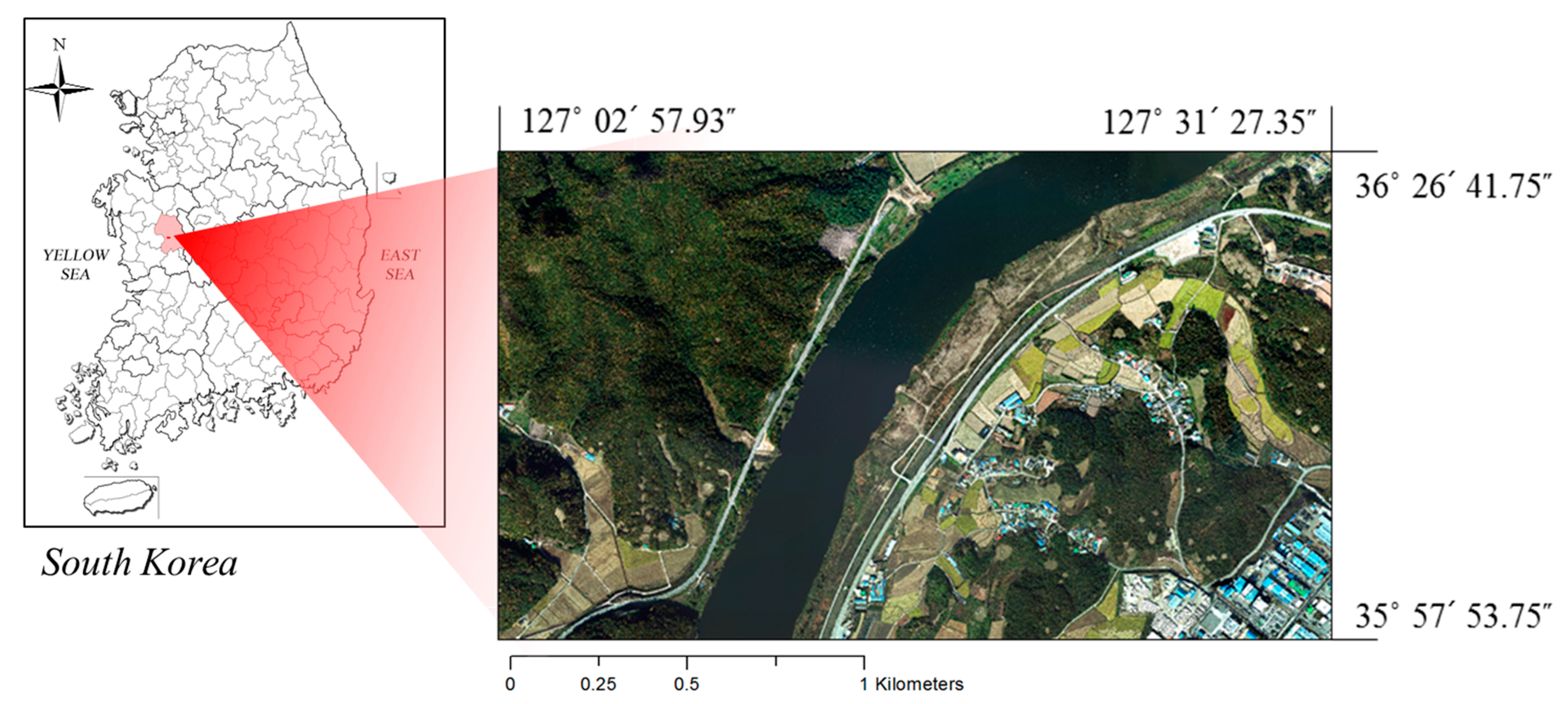
The study area is located in Gongju province, South Korea, as shown in
Figure 1. Gongju is 864.29 km
2 in area, about 0.95% of the total area of South Korea (99,407.9 km
2). The area of cultivated land is 185.82 km
2, accounting for 19.76% of the total area. Forests constitute 70% of the area and there are many hilly mountainous areas of 200–300 m above sea level. The average temperatures are around 11.8 °C in spring, 24.7 °C in summer, 14.0 °C autumn, and −0.9 °C in winter. The average annual precipitation is 1466 mm. The soils are loamy soils and clay loams and at the bottom it has sand soils. The image of the study area covers a 3.25 km
2 area that is 2344.8 m in length and 1385.76 m in width.
The RGB aerial orthophoto shows the spatial distribution of forests in the study area. Most forests are present on steep-sloped mountains and the types of forest include coniferous/broad-leaved forests and artificial/natural forests.
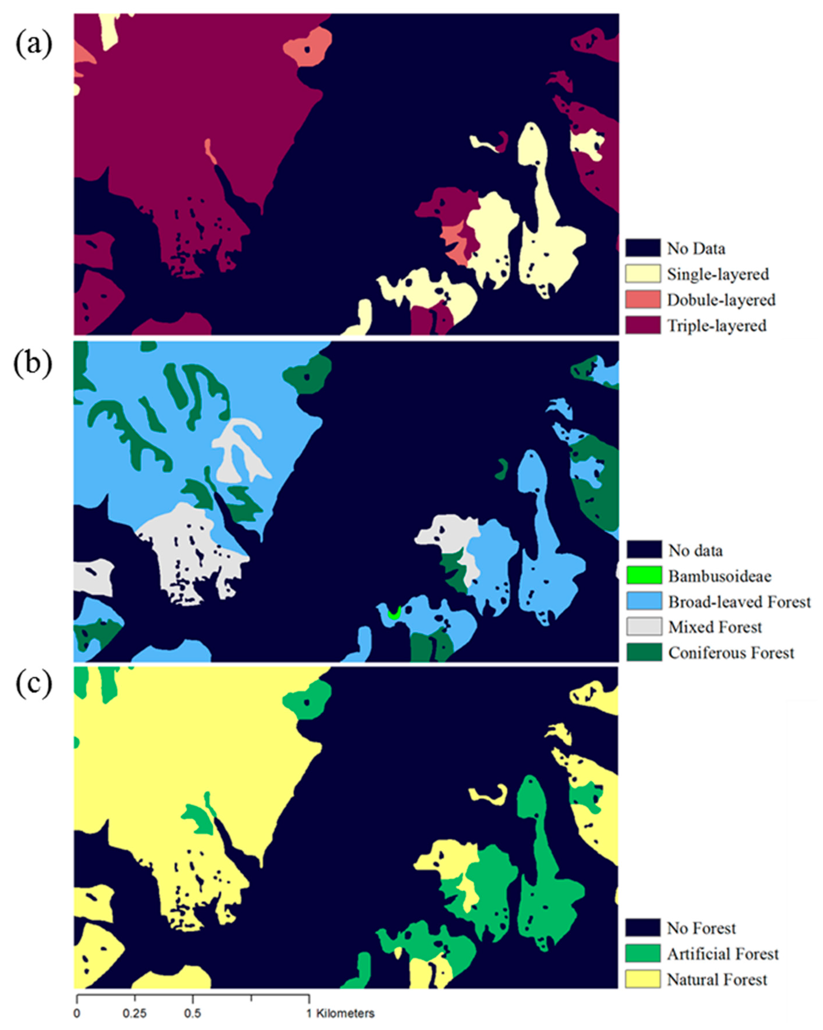
Figure 2 shows the three types of forest classification map that are based on vertical structure, dominant species’ leaf type, and whether the forest is natural or artificial. These maps were classified based on field survey measurements collected as a part of the Korean 3rd natural environment conservation master plan. The measurements were collected for the whole country over a period of six years from 2006 to 2012. The field survey of the study area was performed in 2009. The fourth masterplan started in 2014 and is due to be completed in 2018. The database construction for the fourth masterplan has not been completed.
Figure 2a shows that triple-layered forests were dominant in the study area, and hence the natural forests are shown to be dominant in
Figure 2c because the artificial forests are generally single- or double-layered. The study area includes a variety of different forest types including: (i) single-, double-, and triple-layered forests (
Figure 2a); (ii) broad-leaved, coniferous, and mixed forests (
Figure 2b); and, (iii) natural and artificial forests (
Figure 2c).
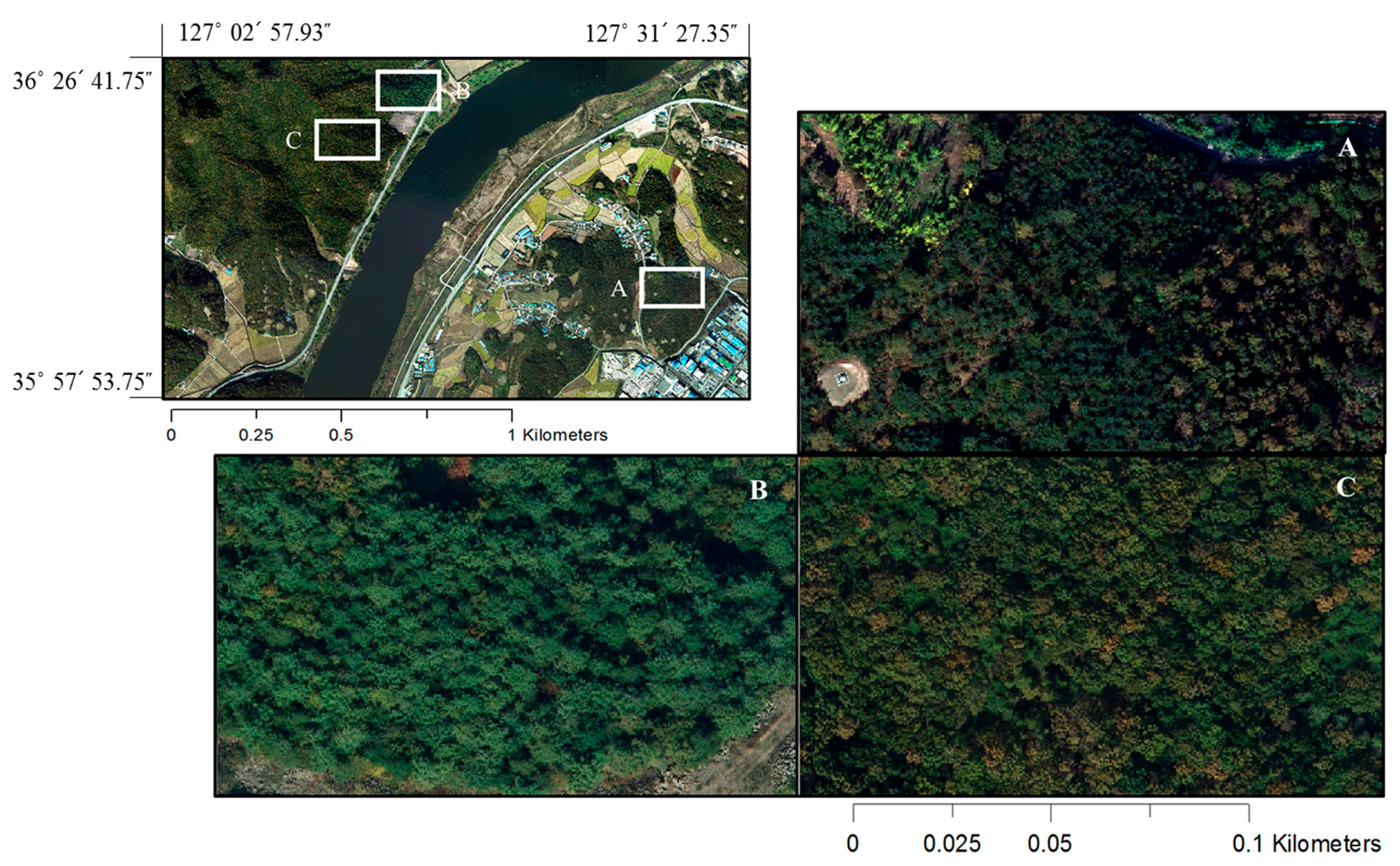
Figure 3 shows examples of single-, double-, and triple-layered forests.
Figure 3a shows an example of a single-layered forest. The forest is a chestnut plantation that the image shows to have been uniformly planted. Thus, it can be understood that it is an artificial forest. In
Figure 3b, the image was acquired from a double-layered forest. It is a coniferous forest and the nut pine is dominant. The red reflectance value of coniferous trees was lower than that of broad-leaved trees based on analysis of the RGB image. This confirmed that the brightness is dependent upon species. Considering that coniferous forests are mainly single- or double-layered, species identification could be an important part of the classification of vertical structure.
Figure 3c shows an example of a triple-layered forest. The forest is broad-leaved and oak is dominant tree type. Natural forests are a mixture of various species, and may contain coniferous and broad-leaved trees. Therefore, it is expected that it will be more useful to analyze height differences between trees rather than the identification of tree species in the classification of triple-layered forests. As mentioned above, single- and double-layered forests are mostly artificial forests. Artificial forests in the study area include broad-leaved forests, such as the chestnut tree forest, as well as coniferous forests such as the nut pine forest.
The RGB orthophoto was obtained using a DMC II airborne digital camera at an altitude of 1300 m (above sea level) with a redundancy rate of 63% in October 2015. The low-resolution RGB and high-resolution panchromatic (PAN) images were merged to create a high-resolution RGB image. The high-resolution RGB image was then orthorectified and mosaicked. The final mosaicked RGB orthophoto was used for this study. The ground sample distance (GSD) of the orthophoto was 12 cm in both the line and pixel. The lidar point cloud was acquired with an ALTM Gemini167 at an altitude of 1300 m (above sea level) in October 2015 with 2.5 points per square meter in the lowlands and 3~7 points per square meter in the mountain area. The difference in the point density occurred because the overlap rate of the lidar sensors is different between mountainous and non-mountainous areas. Points from terrain was classified from the Lidar point cloud, the DTM with the GSD of 1 m was created from the terrain-derived points. On the other hand, points from trees were extracted, and then the DSM with the GSD of 1 m was produced from the tree-derived points. The terrain- and tree-derived points were extracted by using the commercial software Global Mapper. The height difference map was generated by subtracting DTM from DSM. The height difference map is related with several tree parameters, including the height and density of trees, etc. That is, the pixel values in the height difference map are not tree height, but are closely related with tree height.
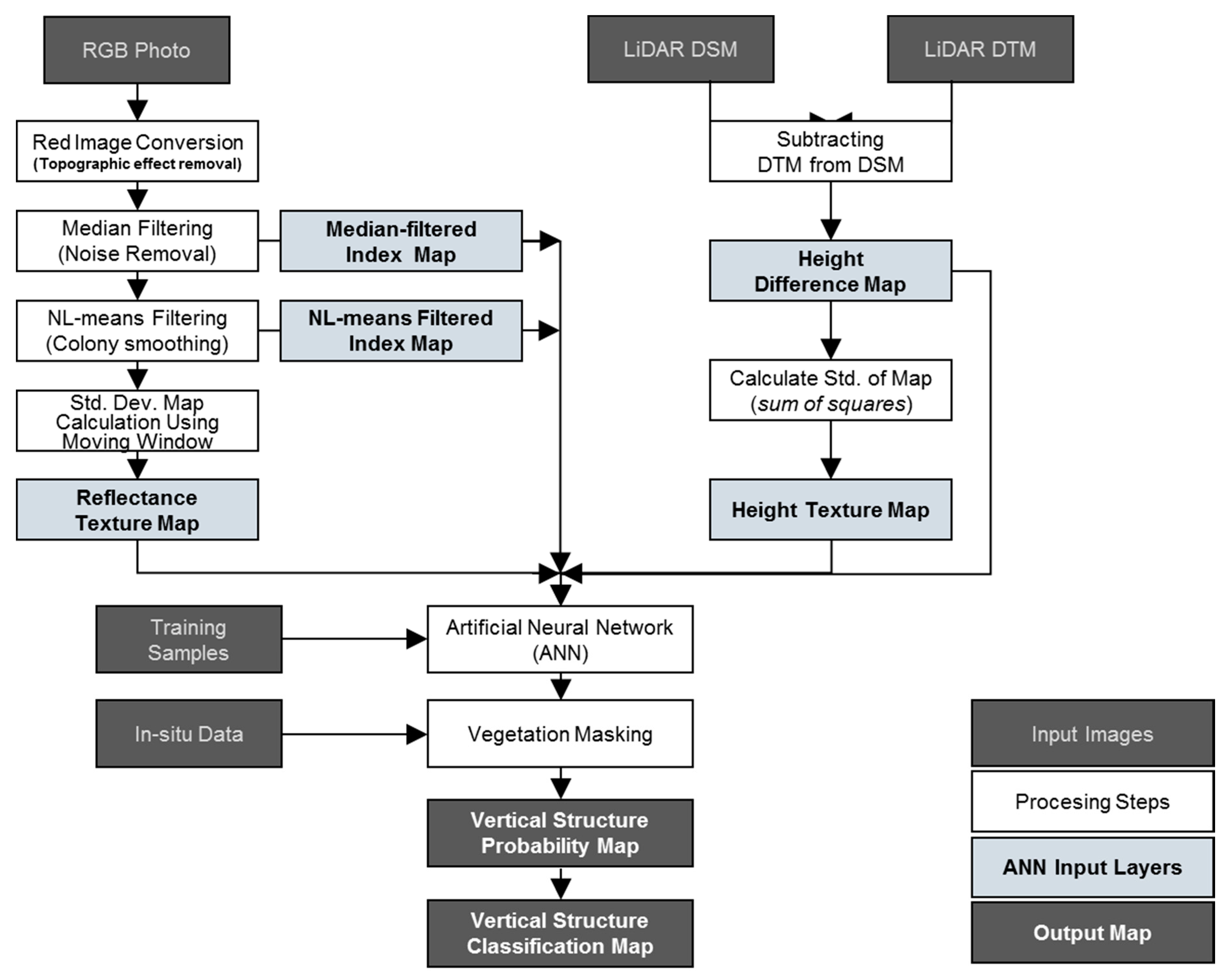
3. Methodology
In this study, we produced five input maps that were resampled to 0.48 m GSD from high-resolution RGB imagery and lidar DSM and DTM data. The three maps from the RGB image include: reflectance values from each tree, reflectance values from each colony, and the variance of reflectance values (i.e., a texture map of reflectance). The two maps from lidar data reflect the tree height of each individual species, and the variance of the height values. We classify forest vertical structure by applying an Artificial Neural Network (ANN) to the five maps. An ANN is a large network of extremely simple computational units that are massively interconnected with nodes and processed in parallel. In this study, a multi-layer artificial neural network was used. It contains three layers: an input layer, a hidden layer, and an output layer, and each layer is composed of nodes. Each node has a weight, which is adjusted from randomly generated initial values through the iterative experiment to obtain the most reasonable output [
25,
26].
Figure 4 shows the detailed workflow used to classify the forest vertical structure from RGB orthophoto and lidar data using a machine learning approach. The image processing steps such as median, NL-means filtering, texture calculation was implemented by using C language, the MATLAB software was used for the ANN processing, and ER-mapper was used to display input and output maps.
3.1. Generation of Input Data from RGB Imagery
Vegetation has different reflectance values on remotely sensed imagery because different species have different leaf pigments. When these characteristics were determined from RGB imagery, the needle-leaf forest was brighter than the broad-leaf forest on the converted red image (Median-filtered Index Map). To analyze the optical imaging characteristics of each colony’s vegetation, a normalized index map was produced. First, the initial RGB imagery (0.12 m GSD) has a deep shadow due to topographic effects that should be reduced. The shadow effect appears in both the red and green images. Thus, an index map was used instead of the red or green images. The index map is generated in two steps: (i) the red image is converted using the mean and standard deviation of the green image; and (ii) the ratio of the difference between the red and green images and the summation of the red and green images is calculated. This conversion reduces the topographic shadow artefact very effectively. The converted red image (
) was calculated using:
where
i and
j are the line and pixel, respectively,
R is the red image,
and
are the means of the green and red images, and
are
are the standard deviation of the green and red images. The normalized index map (
NI) was defined using:
where
G is the green image.
The index map contains noise from the crown. Since it can degrade the accuracy of the ANN analysis, we applied a median filter with a kernel size of
pixels to reduce the noise. The median filtered index map was used as part of the input data for the ANN. To determine each colony’s overall reflectance, we resampled the median-filtered index map to a spatial resolution of 48 cm and applied a NL-means filter with a kernel size of
. The NL-means filter is a powerful smoothing filter that preserves the edges of objects. The NL-means filtered index map represents the overall reflectance of a forest vegetation colony. The third input map from the RGB image indicates the spatial texture of the reflectance values. If a colony has a double- or triple-layered forest vertical structure, it must have several species and the species’ reflectance values must be mixed. Thus, if a colony contains various species, the spatial texture of the reflectance would be rough. On the contrary, if only a few species are present such as in an artificial forest, the spatial texture would be smooth. The reflectance texture map is generated by calculating the standard deviation of the difference between the median-filtered and NL-means filtered maps using a moving window of
.
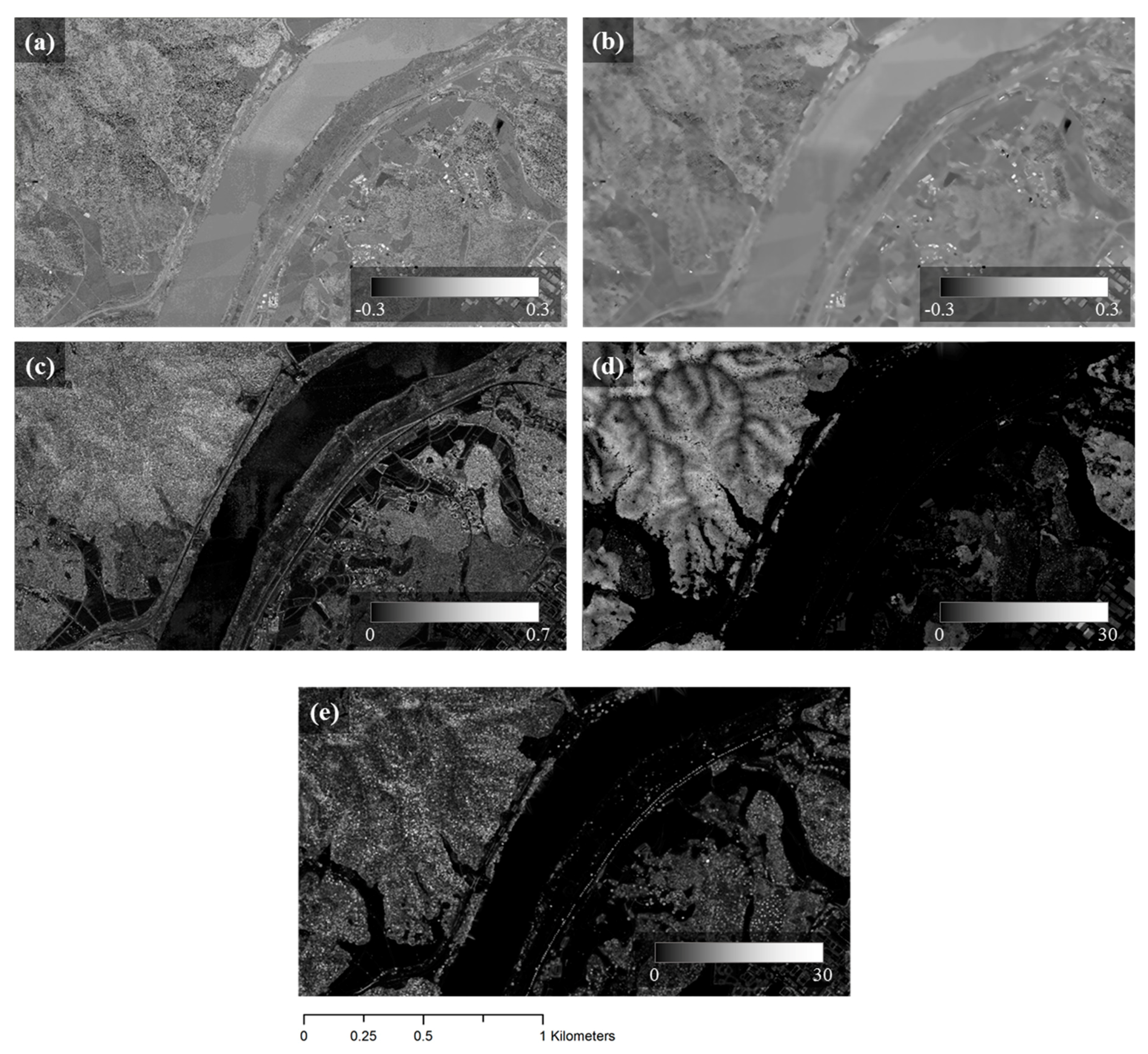
Figure 5 shows the three input layers used for the ANN analysis. To ensure that the topographic effect was mitigated in the median-filtered index map from
Figure 5a, it was compared with
Figure 1. As shown in
Figure 5b, the NL-means filtered index map was smoothed with well preserved object edges. The smooth or rough texture of the surface reflectance map can be recognized from
Figure 5c. The water surface had lower values while the forest areas had higher texture values.
3.2. Generation of Input Data from Lidar Data
Forest vertical structure is highly related to tree height. This is because the criteria for classification of canopy, understory, and shrub layers in a forest inventory are tree species and tree height. Two input layers were generated from the lidar data (initially 1 m GSD, but resampled to 0.48 m GSD): a height difference map and a height texture map. The height difference map was generated by subtracting the DTM from the DSM. The DSM is a kind of digital elevation model (DEM) that represents the Earth surface including features such as building, trees, and houses. The DTM is also a kind of DEM, but it only represents the Earth’s terrain and excludes the natural and manmade features. Thus, the height difference map shows the height of the natural and manmade features, including the tree height Pixel values in the height difference map are not direct measurements of tree height, but a close approximation.
The height difference map was used for the ANN analysis. Since the triple- or double-layered forests have various tree species, the variance of the tree height in a colony would be uneven and the standard deviation of height difference in a colony can be large. The calculation of the height texture map from the lidar data is performed by two processing steps. In the first step, the height difference map is smoothed using a NL-means filter with the kernel size of
pixels. The second step involves calculating the standard deviation of the difference between the height difference map and the NL-means filtered height difference map using a moving window of
pixels. This map is used for the ANN classification processing.
Figure 5d shows the height difference map. The relative height difference among trees can be recognized from
Figure 5d.
Figure 5e shows the height texture map that indicates the spatial variance in tree height.
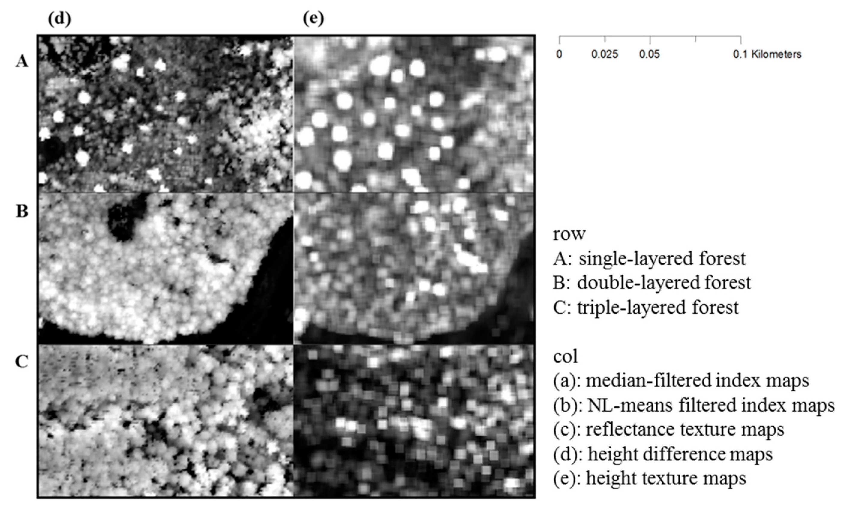
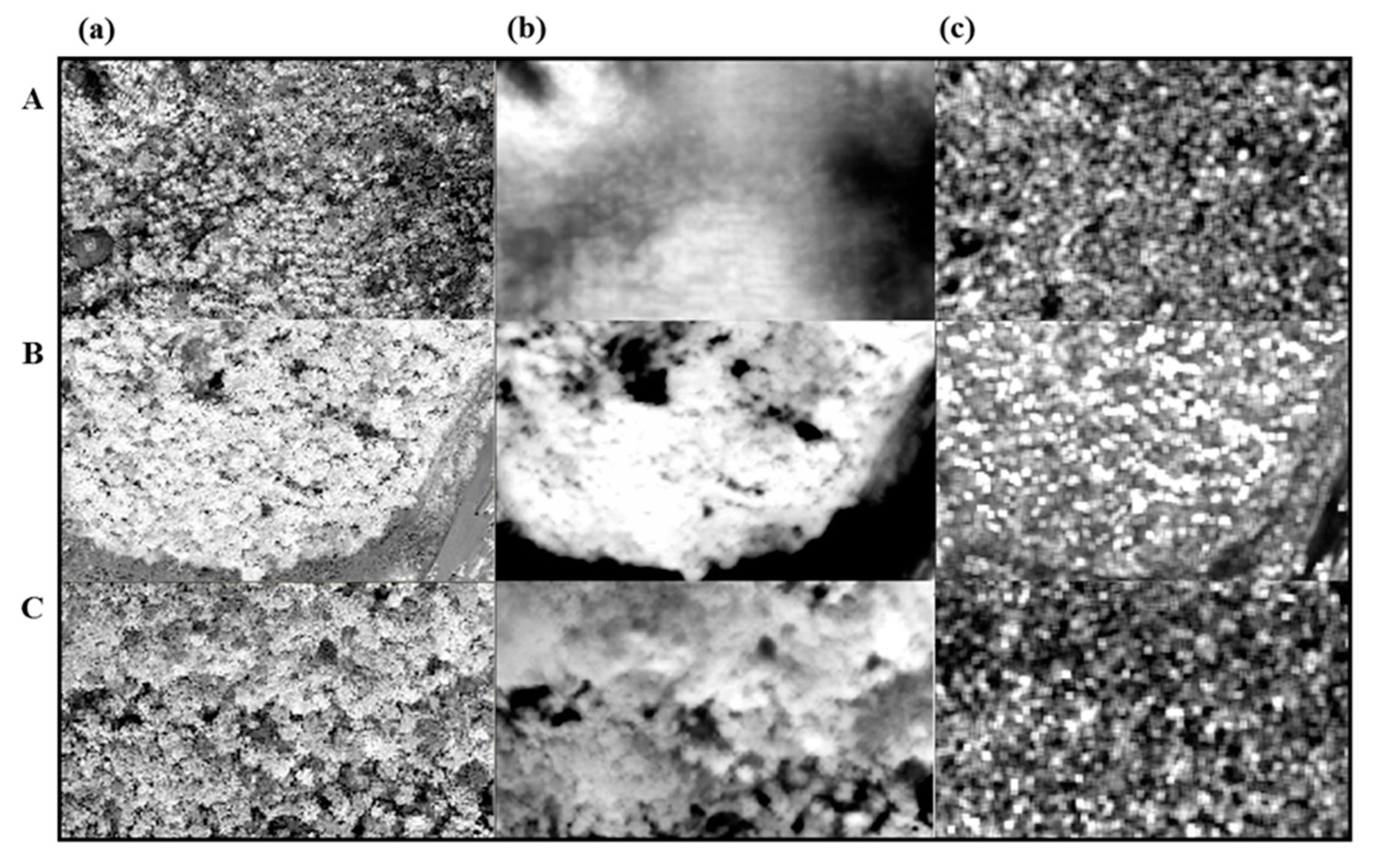
Figure 6 shows the characteristics of the five input layers used for the ANN. The areas in the boxes labeled A, B, and C in
Figure 6 are representative of single-, double-, and triple-layered forests, respectively. The dominant species in the area under box A is chestnut tree and the area is a broad-leaved and artificial forest. The area under box B includes nut pine trees as the dominant species and is a coniferous and artificial forest. The dominant species in the area under box C is oak tree and the area is a broad-leaved and natural forest. The nut pine (box B in
Figure 6) was the brightest of the forests among the reflectance index maps. The reflectance texture maps in the single- and double-layered forests were smoother than the triple-layered forest. In box A of
Figure 6d, there are some individual trees in the artificial forest that appear as bright patches. These trees show different reflectance values on the RGB and median-filtered index maps as compared with other trees in the same community and appear to be a different species. They show odd values on the maps from the lidar data as well. The brightest parts of the Height Texture Map (
Figure 6e) are where the standard deviation was high.
4. Results and Discussion
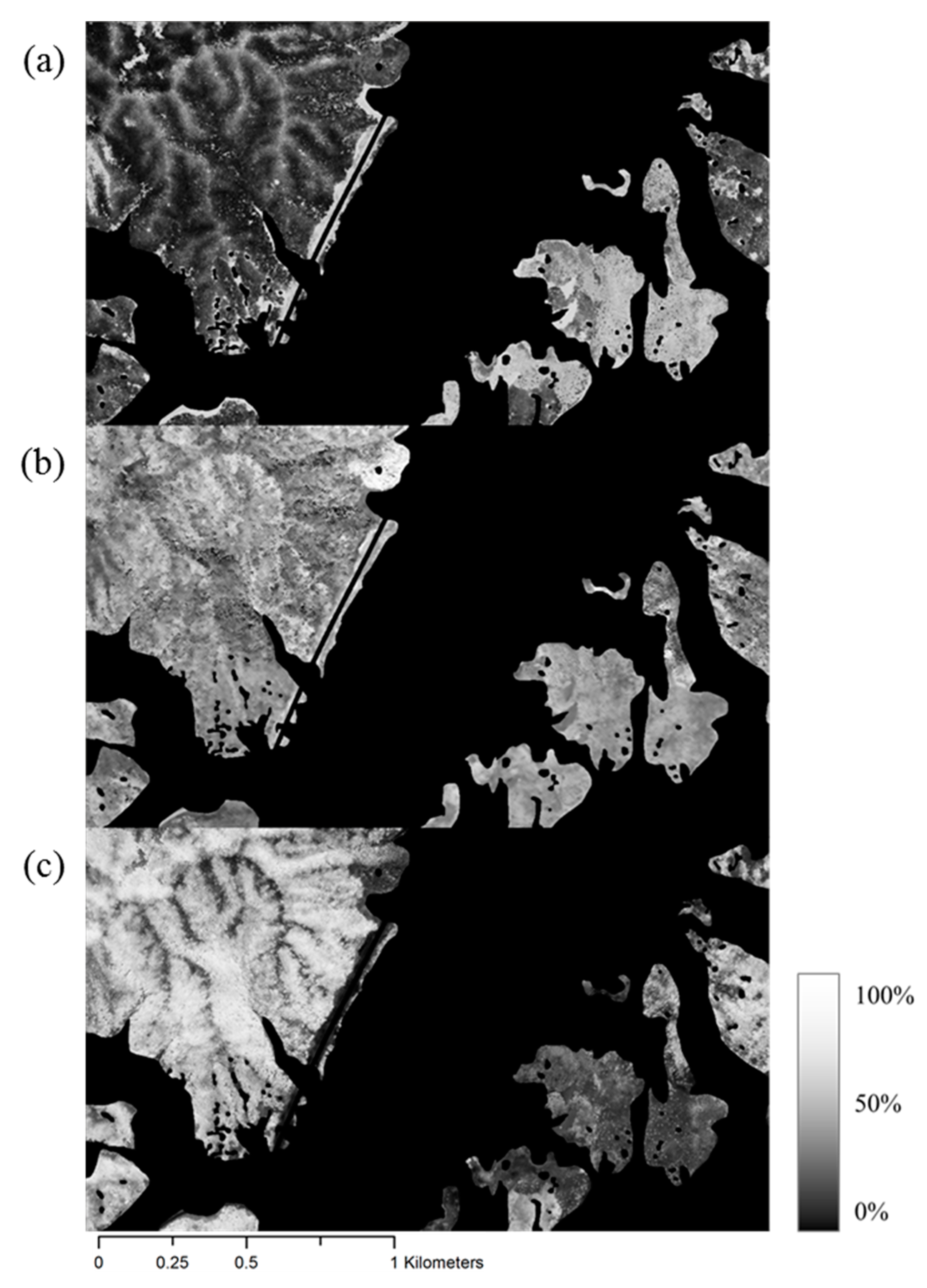
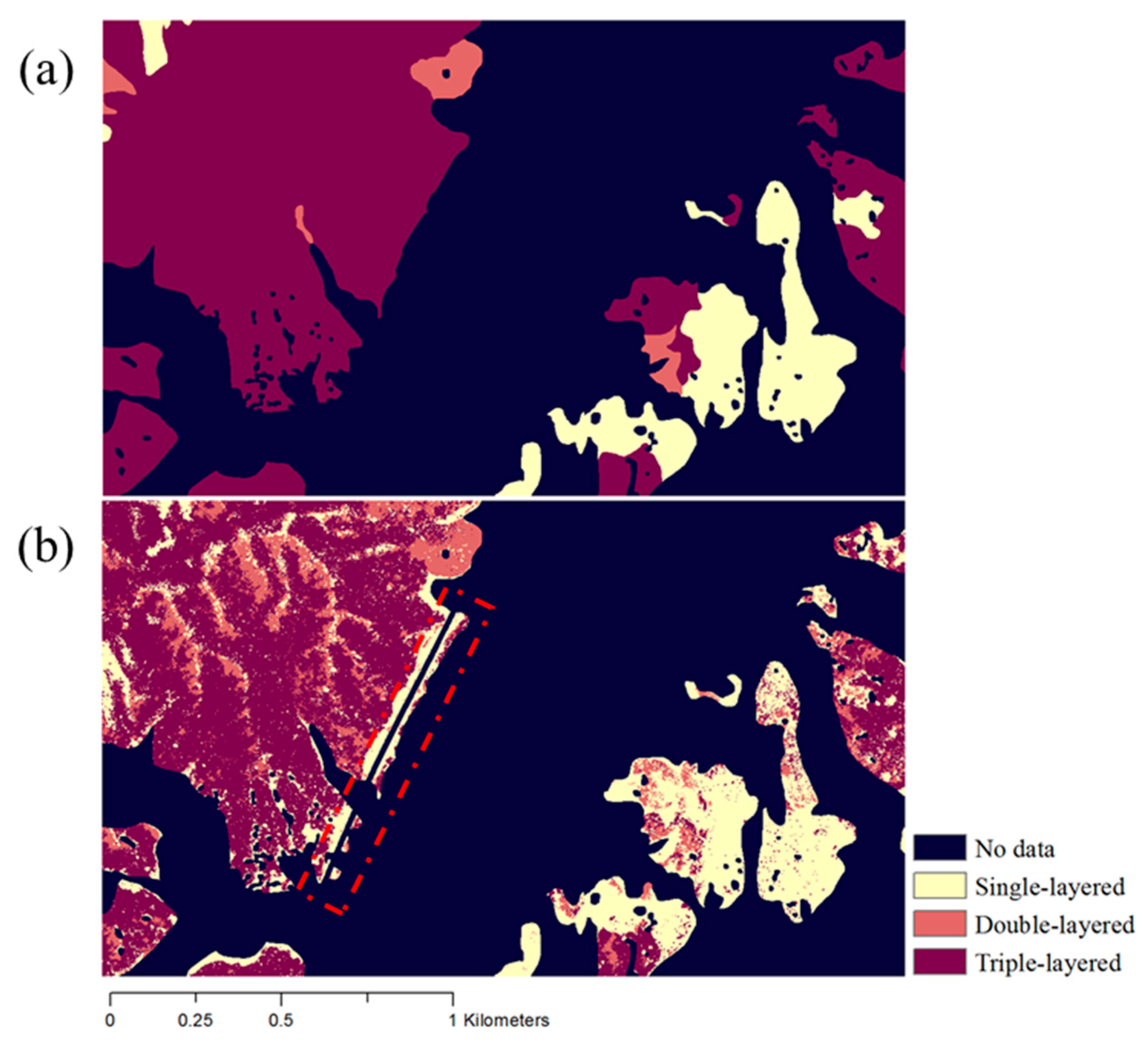
Figure 7 shows probability maps of the single-, double-, and triple-layered forests generated using the ANN and the five input layers. The ANN is a pixel-based analysis that calculates a probability of an event happening, and the brightness values represent probabilities. Training samples of ten thousand pixels were selected for the single-, double-, and triple-layered forests from field survey measurements. The non-vegetation areas and the road (red-dotted box in
Figure 8) were masked out. The ANN determined the weighting factors from the five input layers.
Table 1 summarizes the weighting factor for each input layer.
From the single-, double-, and triple-layered forests shown in
Figure 7a–c, a final forest structure classification map was produced by selecting the highest value from the probability maps of the single-, double-, and triple-forests.
Figure 8 shows the ANN-classified forest structure map and the field forest structure map for comparison. The red-dotted box in
Figure 8b was classified as single-layered forest using the ANN approach, but the field measurements recorded it as triple-layered forest (e.g., compare
Figure 8a,b). The field measurements have low spatial sampling because most forests in Korea occur in high mountainous regions. This discrepancy was caused by the spatial resolution differences. The forest vertical structure classes between the ANN approach and field measurement were compared and the results are summarized in
Table 2. In
Table 2, the number denotes the number of pixels. The classification accuracies of the single-, double-, and triple-layered forests were 82.84%, 56.56%, and 69.03%, respectively. The overall accuracy was 71.10%.
For the sections with low classification accuracy, the reasons for the misclassification need to be investigated. However, the overall accuracy of the classification is relatively high, considering that it is difficult to classify the vertical structure of a mixed-species forest using remotely-sensed data [
17]. Our results show that it is possible to classify the forest vertical structure using remotely-sensed data. Several discrepancies were identified and the causes determined. The triple-layered coniferous colonies on the ridge of the mountain were mostly classified as double-layered coniferous forest. This was due to the ANN classification being strongly influenced by the dominant species. The red-dotted box in
Figure 8 is a roadway, which was classified as triple-layered forest in the field measurement data collected in 2009. However, a single-layered forest exists in the roadway when we checked it in the field in 2015 RGB imagery. The road was constructed before 2009. In this case, the ANN approach performed better than the field measurements due to a low spatial resolution of the field survey sampling. However, we should be aware that the time lag between airborne images and field survey data can result in differences such as boundary changes or forest succession. The discrepancy between the ANN and field measurement classifications was very high in the areas of double-layered forest (
Table 2). This is because the double-layered forest is composed of a canopy layer and an understory or shrub layer, and it was very difficult to distinguish from the other vertical structures using the aerial orthophoto and lidar data. Even though using remotely-sensed data and an ANN has some limitations, the approach could be very useful to classify forest vertical structure, because it has a better spatial resolution and is more time- and cost-effective. One other issue was that the RGB image used for this study was created through image tiling by a vendor. The left side of the image (
Figure 8b), is more comparable to the field survey data (
Figure 8a) than the right side. The reason may be due to a slight difference in color when tiling several raw images to process one orthophoto. Therefore, in future studies, it may be better to use raw image data or high resolution satellite image, which have the same photographic conditions over a single image area.
There is much research on the internal structure of forests using dense lidar data [
27], but this method is limited due to the high cost of investigating large areas. Since the forests of Korea comprise a variety of species, it has been difficult to apply the methods of previous studies that identified stratification in coniferous forests composed of similar species [
28]. Therefore, the novelty of the approach used in this study is that it can estimate and classify the complex inner structure of a forest with simple remotely-sensed data.
5. Conclusions
Forest vertical structure one element that represents the vitality of a forest. In general, the forest inventory has been investigated through field surveys. Korea Forest Service currently uses the aerial orthophotos to survey the forests, but it is very difficult to understand the infrastructure of the forests using the remote sensing images because of the cost. Intensive lidar data and aerial orthophotos were used because the orthophotos can just image the forest canopy. Thus, the field survey is inevitable in order to understand the stratification of forest.
In this study, forest vertical structure was classified by using the ANN approach from aerial orthophotos, and lidar DTM and DSM. A total of five input layers were generated from these datasets: (i) a median-filtered index map; (ii) a NL-means filtered index map; (iii) a reflectance texture map; (iv) a height difference map; and (v) a height texture map. Using these maps, a forest structure classification map was generated with the ANN. The classification accuracies of the single-, double-, and triple-layered forests were 82.84%, 56.56% and 69.03%, respectively. The overall accuracy was 71.10%. The accuracy seems good considering that it is not easy to detect the under layers of a mixed broad-leaf and conifer forest from the remotely sensed data. The ANN approach has a better spatial resolution, is a more time- and cost-effective procedure for mapping forest vertical structure. Future studies should consider the effect of time gaps between datasets, and include maps with more detailed information related plant growth such as soil, sunlight, and species characteristics.


