Contrast-Enhanced Ultrasound Imaging Based on Bubble Region Detection
by
Yurong Huang
1,†, 
Jinhua Yu
1,2,3,*,
Yusheng Tong
3,4,†,
Shuying Li
1,
Liang Chen
3,4,*,
Yuanyuan Wang
1,2 and
Qi Zhang
5 1
Department of Electronic Engineering, Fudan University, Shanghai 200433, China
2
Key Laboratory of Medical Imaging Computing and Computer Assisted Intervention of Shanghai, Shanghai 200433, China
3
Institute of Functional and Molecular Medical Imaging, Fudan University, Shanghai 200030, China
4
Department of Neurosurgery, Huashan Hospital, Fudan University, Shanghai 200030, China
5
School of Communication and Information Engineering, Shanghai University, Shanghai 200444, China
*
Authors to whom correspondence should be addressed.
†
Those authors contributed equally to this work.
Appl. Sci. 2017, 7(10), 1098; https://doi.org/10.3390/app7101098
Submission received: 4 September 2017
/
Accepted: 18 October 2017
/
Published: 24 October 2017
(This article belongs to the Special Issue Ultrafast Ultrasound Imaging)
Abstract
:The study of ultrasound contrast agent imaging (USCAI) based on plane waves has recently attracted increasing attention. A series of USCAI techniques have been developed to improve the imaging quality. Most of the existing methods enhance the contrast-to-tissue ratio (CTR) using the time-frequency spectrum differences between the tissue and ultrasound contrast agent (UCA) region. In this paper, a new USCAI method based on bubble region detection was proposed, in which the frequency difference as well as the dissimilarity of tissue and UCA in the spatial domain was taken into account. A bubble wavelet based on the Doinikov model was firstly constructed. Bubble wavelet transformation (BWT) was then applied to strengthen the UCA region and weaken the tissue region. The bubble region was thereafter detected by using the combination of eigenvalue and eigenspace-based coherence factor (ESBCF). The phantom and rabbit in vivo experiment results suggested that our method was capable of suppressing the background interference and strengthening the information of UCA. For the phantom experiment, the imaging CTR was improved by 10.1 dB compared with plane wave imaging based on delay-and-sum (DAS) and by 4.2 dB over imaging based on BWT on average. Furthermore, for the rabbit kidney experiment, the corresponding improvements were 18.0 dB and 3.4 dB, respectively.
1. Introduction
Ultrasound contrast agents (UCAs) [1,2] are a type of diagnostic reagents that typically consist of gas-filled microbubbles with a diameter ranging from 1 to 10 μm. The microbubbles are filled with low solubility gas and are coated with a shell to prevent the microbubble from dissolving. UCAs are injected intravenously into the body and are considered safe for use in humans.
UCAs have been used clinically since the 1980s [1]. Ultrasound contrast agent imaging (USCAI) [3] has generated increased attention in recent years. As a result of the compressibility of microbubbles and the large acoustic impedance difference between them and the surrounding tissue, USCAI can greatly improve the contrast (CR) and contrast-to-tissue ratio (CTR) of a clinical ultrasound image. The detection rate, sensitivity, and specificity with which small lesions can be detected can therefore be greatly increased [4,5].
Plane wave imaging (PWI) [6] has a great advantage over traditional B-mode imaging for USCAI. First, PWI can significantly reduce the destruction of microbubbles due to its low mechanical index. Second, PWI can track fast-moving microbubbles due to its high frame rate. However, poor imaging quality limits the clinical application of PWI.
A large proportion of novel USCAI technologies [7,8] appears to focus on the improvement of PWI imaging quality. Most of these existing methods enhance the image CTR by utilizing the abundant harmonic signals produced by UCAs. Generally speaking, the mainstream USCAI technologies can be classified into two categories: pulse coding [9] and bubble wavelet transformation (BWT) [10,11].
Pulse coding focuses on the transmitting end as it either changes the number of the transmit pulse, transmit phase, transmit frequency, or transmit amplitude. Pulse inversion (PI) [12], amplitude modulation (AM) [13], chirp encoded excitation [14], and Golay\encoded excitation [15] are typical representatives of such methods. Since the response of UCA is represented as harmonic signals while that of tissue represents predominantly fundamental signals, the tissue signal can be removed by PI and AM technology. Chirp-encoded excitation emits a long sequence with the frequency variation over time. Studies have shown that chirp excitation has the ability to strengthen the harmonic signals and lower the sub-harmonic generation threshold [16]. However, the matched filter is needed in the receiving end to decode the signal, which adds complexity.
Bubble wavelet transformation (BWT) is a novel type of USCAI technology proposed by Wan et al. [10,11]. BWT is utilized to analyze the correlation between the mother bubble wavelet and the received radio frequency (RF) signals. The constructed bubble wavelet obtained by simulating the microbubble model was highly correlated with the signals of microbubbles and has few similarities with the signals from surrounding tissues. The ability of BWT to enhance the imaging CTR has been validated by in vivo experiments. A mother wavelet was constructed by microbubble model simulation. The RF signals were then processed by the continuous wavelet transformation and a series of coefficient matrices was obtained. A better image quality and an enhancement of 6.0 dB in CTR can be obtained with BWT [11] while ensuring the high frame rate of PWI.
Both the pulse coding and BWT improved the CTR in the time-frequency domain. Under a low mechanical index, tissue produces a predominantly linear response and, thus, it is feasible to distinguish tissue and UCA according to their frequency components. The non-linear distortion of waveforms and the spectrum overlap between the tissue and UCA is an unfavorable factor.
In this paper, we take the tissue and UCA differences in both the frequency and spatial domains into consideration. PWI was used to improve the imaging frame rate and ensure the stability of UCA. A bubble wavelet based on the Doinikov model was firstly constructed. BWT was then applied to strengthen the UCA region and weaken the tissue region. Following this, the bubble region was subsequently detected by utilizing the combination of eigenvalues and eigenspace-based coherence factor (ESBCF). The residual tissue signal could be further suppressed, and a higher CTR was obtained.
2. Materials and Methods
2.1. Frequency Domain
2.1.1. Bubble Wavelet Transformation (BWT)
With the rapid development of ultrasound molecular imaging, about a dozen of microbubble models [17] have been proposed. The dynamic behavior of a single microbubble under different ultrasound fields can be predicted with the help of these models. BWT applied the microbubble model to USCAI, where a novel mother wavelet named as a bubble wavelet was constructed based on the simulation results of the microbubble model.
The expression of BWT in the time domain can be described as:
where x(t) is the signal to be processed; φ(t) is the bubble wavelet; φ() is the function of the bubble wavelet after translation and scaling; a is the scale factor; b is the time-shifting factor; and superscript * denotes the conjugation operation.
In fact, BWT is the convolution operation of the bubble wavelet under different scale factors with the signal to be processed. The result of BWT is a series of wavelet coefficients. These coefficients, namely the function of the mother wavelet and the scale factor, illustrate the correlation between the bubble wavelet under a certain scale and the received signal. Due to the similarity of the frequency spectrum of the bubble wavelet and the UCA echoes, as well as the dissimilarity between this and the tissue echoes, the tissue signal can be weakened and the UCA signal can be strengthened after BWT.
In the application of BWT, the choice of the bubble wavelet and the scale factor are two key elements [18,19] that determine the image quality to a large extent. A more significant effect of CTR improvement can be achieved if the spectrum of the bubble wavelet is highly matched with that of UCA. The scale factor is another key issue. The scale resulting in the highest CTR is selected as the optimal factor.
2.1.2. Construction of Bubble Wavelet
Among the existing models, the Doinikov model [20] focuses on microbubbles with phospholipid shells. The Doinikov model has been proven to predict the ‘compression-only’ behavior [21] of Sonovue very well. It is commonly accepted that its spectrum is closer to that of the Sonovue microbubble and is the optimal choice for the bubble wavelet [17,22].
The Doinikov model can be described as:
where ρl = 1000 kg/m3 denotes the density of the surrounding liquid; P0 = 101,000 Pa as the atmospheric pressure; γ = 1.07 as the gas thermal insulation coefficient; R0 = 1.7 μm as the initial radius of microbubble; R is the instantaneous radius of microbubble; R′ is the first-order time derivative of R, with essentially R′ = dR/dt and R″ = d2R/dt2; σ(R0) = 0.072 N/m as the initial surface tension; χ = 0.25 N/m as the shell elasticity modulus; ŋl = 0.002 PaS as the liquid viscosity coefficient; k0 = 4 × 10⁻⁸ kg and k1 = 7 × 10⁻¹⁵ kg/s as the shell viscosity components; α = 4 μs as a characteristic time constant; and Pdrive(t) is the driving ultrasound.
The pressure scattered by the microbubble can be expressed as:
where d denotes the distance from the center of the microbubble to the transducer.
Following this, the bubble wavelet can be obtained by solving Equations (2) and (3) with the initial condition of R(t = 0) = R0, R′(t = 0) = 0.
2.2. Spatial Domain
Beamforming is an important part of the medical imaging system, and plays an important role in the imaging performance. Delay and sum (DAS) is the basic beamformer with a fixed weight. Its poor image quality promotes the development of adaptive beamformer. The minimum variance (MV) algorithm [23] is the originator of the adaptive beamformer. Eigenspace-based minimum variance (ESBMV) [24] was proposed since the improvement of MV in CR is not obvious.
Based on the observation of the differences between the UCA and the tissue region on the maximum eigenvalues and eigenspace-based coherence factor (ESBCF) index, we proposed a bubble region detection scheme based on the combination of eigenvalue and ESBCF index.
2.2.1. Eigenvalue
In the bubble region detection algorithm, the signal intensity is the most important characteristic. In the theory of ESBMV, the maximum eigenvalue belongs to the mainlobe signals [24]. The signal subspace is comprised of eigenvectors corresponding to the largest few eigenvalues, and the noise subspace is constructed by eigenvectors according to lower eigenvalues. The small eigenvalues tend to represent the noise field and the large eigenvalues represent the signal field [25]. Furthermore, the maximum eigenvalue gives an estimation of the signal power. Zeng et al. proposed a method to detect the signal based on the eigenvalues [26,27,28], which proves that it is practicable to distinguish the UCA and tissue region according to their eigenvalues from the side. Based on the observation of the experiment, we found that the amplitude of the maximum eigenvalue in the UCA region is obviously higher than that in the tissue region.
The eigenvalues are calculated as follows:
The RF signals were divided into several overlapping subarrays. The covariance matrix was computed after spatial smoothing and diagonal loading as follows:
where R is the covariance matrix; k is the time index; M is the transducer elements; M − L + 1 denotes the overlapping subarray number; L is the length of subarray; p is the subarray number; xdp(k ) is the signal after delay; and (·)H is the transposition.
The eigen-decomposition of the covariance matrix was required:
where is the square matrix of eigenvalues in the descending order and U is the eigenvector corresponding to the eigenvalue.
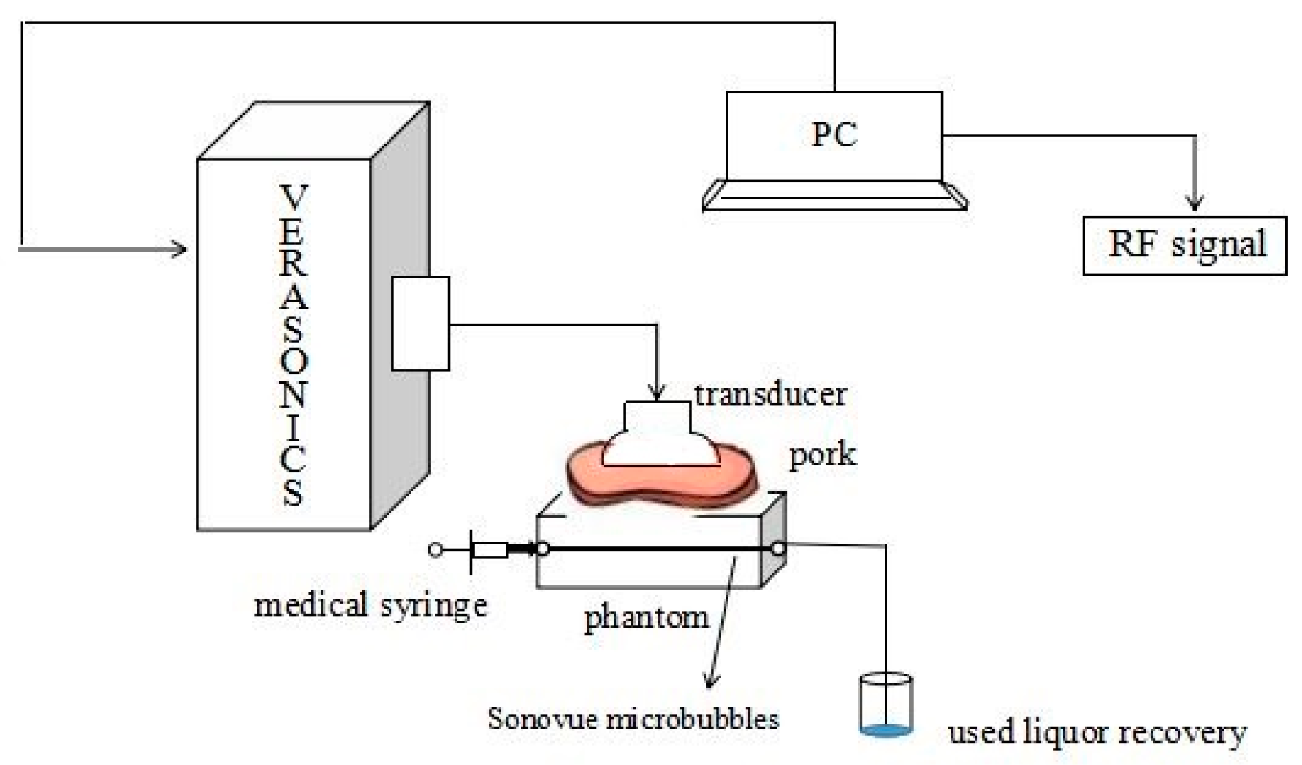
By taking a phantom study as an example, the bubble detection ability of the eigenvalue is explained. The scheme of the phantom experiment is shown in Figure 1. The experiment system includes an ultrasonic research platform Verasonics Vantage 128 (Verasonics, Inc., Kirkland, WA, USA), a linear array transducer (L11-4v), a homemade gelatin phantom, a medical syringe, a tube, a beaker, a computer, Sonovue microbubble (Bracco Suisse SA, Switzerland), and fresh pork.
The phantom is 11 cm in length, 11 cm in width, 6 cm in height, and is made of gelatin. The process of making the phantom is as follows: (1) mix 50 g gelatin granules with 700 mL purified water; (2) heat the mixture for about 10 min until the gelatin particles are completely dissolved in water; (3) glue a plastic tube (whose diameter is 0.5 mm) to the sides of the plastic mold; (4) pour the mixture into the mold; (5) refrigerate the mixture in the freezer for about 3 h; (5) remove the mixture from the mold after the mixture is solidified; (6) draw the plastic pipe out of the phantom. A phantom with a wall-less tube is completed.
The fresh pork (the belly of a pig, 15 mm in thickness, 40 mm in length, and 25 mm in width) was bought from a local meat market on the day of the experiment. Verasonics was used to excite the ultrasound wave and record the RF data. Matlab was used to analyze the RF signal offline. The flowing Sonovue solution (diluted by 1000 times with 0.9% physiological saline) was injected into the pipe by a medical syringe, and the used solution flowed into the beaker. We placed a piece of fresh pork over the phantom. The ultrasonic coupling agent was applied between the pork and the phantom to ensure the signal transmission.
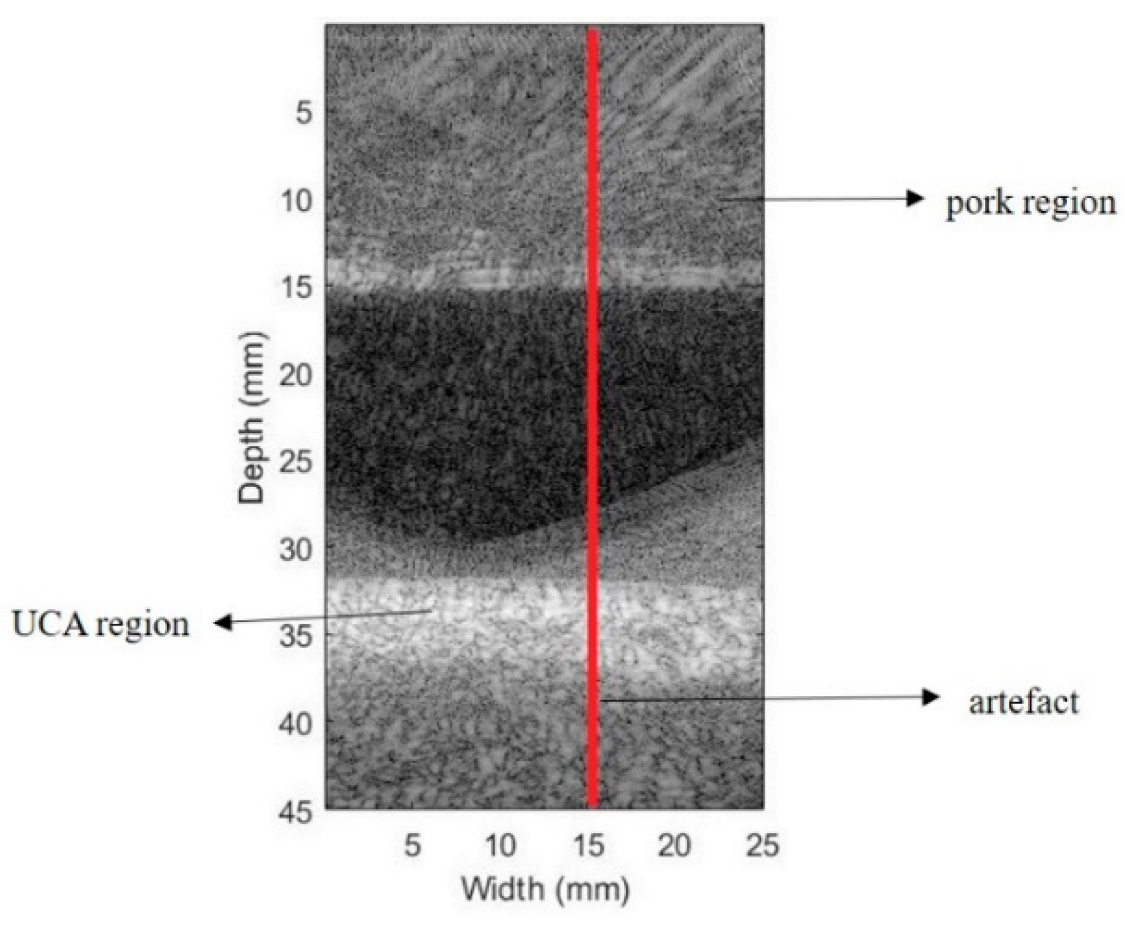
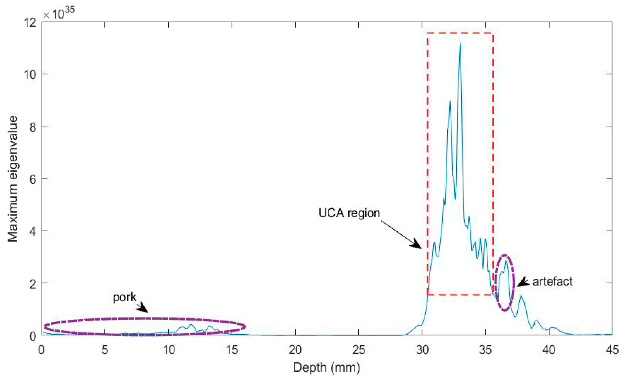
The phantom image beamformed with DAS is shown in Figure 2, where the depth ranging from 0–15 mm is the pork area and that ranging from 30.5–35.5 mm is the bubble area. Taking the area at the width of 15 mm as an example, the maximum eigenvalue curve under different depths is shown in Figure 3. The area enclosed with the red rectangle represents the UCA region. Its maximum eigenvalue is quite large due to the existence of strong scattering signals produced by the UCA. The two purple ellipse areas are the interference region from tissue. For the artefact region, its eigenvalues are partially overlapped with the UCA due to the interference of the strong scattering signals from the UCA. On the other hand, in the pork part, its maximum eigenvalue is much smaller. Hence, we are able to eliminate the pork section preliminarily by setting an eigenvalue threshold. However, the disturbance of the artefact still exists. Thus, we further consider the application of ESBCF to remove the residual disturbance.
2.2.2. ESBCF
Coherence factor (CF) [29] is a type of adaptive weighting method based on the spatial spectrum of array data. In the last several years, a series of improved methods based on CF has been proposed [30]. ESBCF, proposed by Guo et al. [31], combined CF with a covariance matrix. The ability of ESBCF to detect point targets was verified by phantom and simulation experiments.
The description of ESBCF is as follows:
where Rvi = Vi*ViH is the covariance matrix of eigenvector Vi; i is the eigenvector index; and n is the element index.
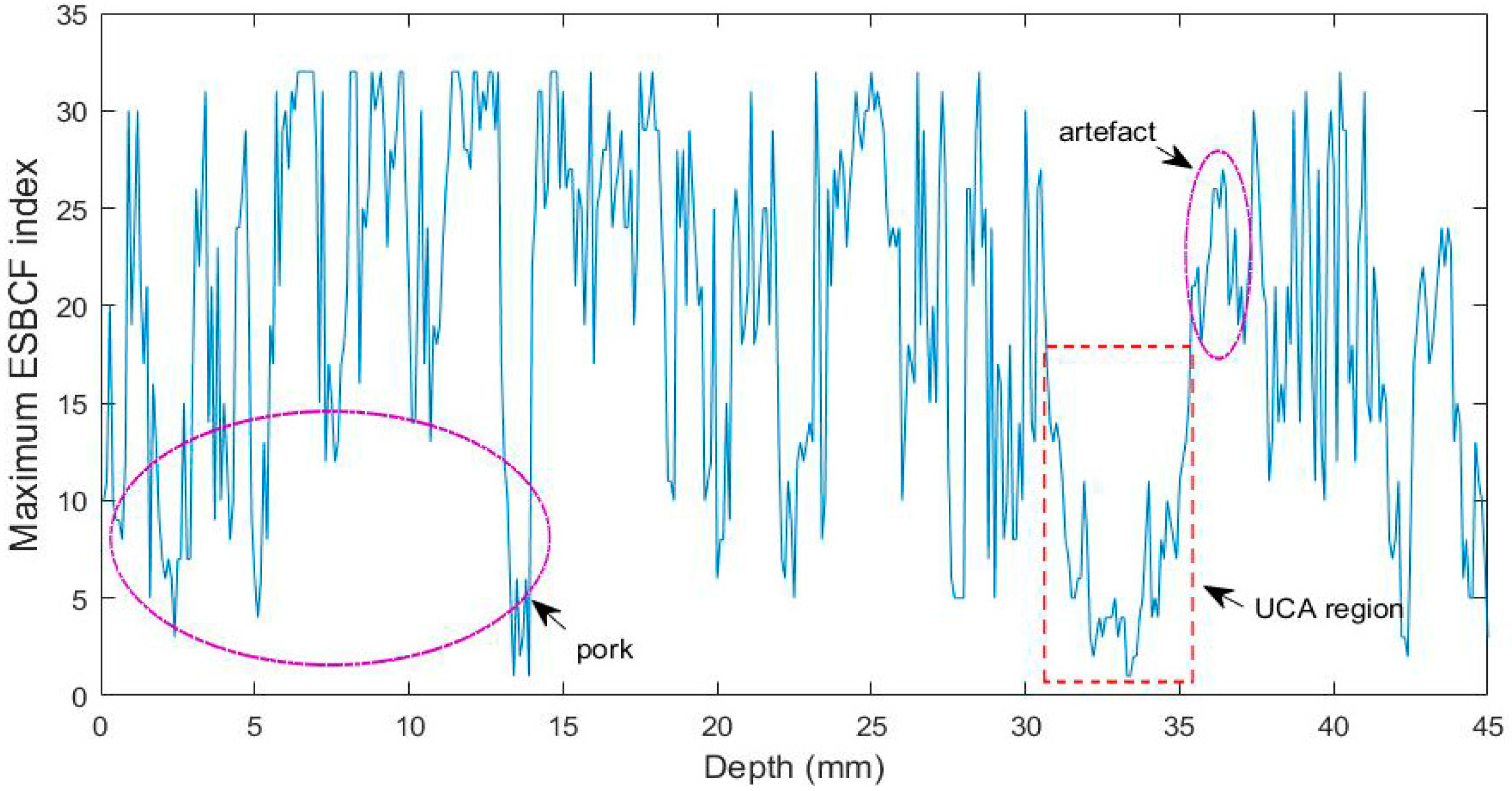
The maximum ESBCF value index curve of each imaging point is shown in Figure 4. For the UCA region, its maximum ESBCF value appears in the first few eigenvectors. In contrast, for the residual upper disturbing section, its maximum ESBCF value appears later. In this present study, the remaining upper interference can be removed by setting a maximum ESBCF index threshold.
2.2.3. Implementation of Bubble Region Detection
The calculation procedure of the bubble region detection method can be summarized as follows:
- (1)
- BWT was first conducted to enhance the UCA signal, and the received RF signal was replaced by the wavelet coefficients under the optimal scale factor.
- (2)
- The covariance matrix was computed according to Equation (4).
- (3)
- The MV weight was obtained by minimizing the array noise output energy, which can be expressed as:where d is the direction vector; and w is the weight vector.
- (4)
- The eigen-decomposition of the covariance matrix was required:where subscript S denotes the signal and subscript P is the noise subspace. The signal subspace is comprised of eigenvectors corresponding to the largest few eigenvalues (α times greater than λ1 or β times greater than λL).
- (5)
- Based on the last step, the maximum eigenvalue and ESBCF for each imaging point was obtained. Following that, we found the maximum ESBCF index.
- (6)
- We set the maximum eigenvalue and ESBCF index threshold to determine whether it is the UCA region or not.
- (7)
- The ESBMV weight comes to:where USU is the eigenvectors of the signal subspace of the detected UCA region.
- (8)
- The region detection output is given by:
- (9)
- The final image can be formed after the signals are enveloped and the logarithmic transformation is applied.
2.2.4. Selection of Optimal Index
Scale Factor
By extending the time-domain expression of BWT to the frequency domain, Equation (1) changes into:
where F denotes the Fourier transform.
In essence, BWT is a set of multi-scale filters that can control the passband by changing the scale factor. The correlation between the scale factor and the central frequency of the passband is as follows:
where F(a) is the central frequency corresponding to the scale factor a and Fc is the initial center frequency of the mother wavelet.
Theoretically, the optimal scale factor should be selected where the corresponding center frequency falls at the second harmonic of the UCA. We verified this hypothesis by traversing each scale factor. The optimal scale factor with different bubble wavelets under different transmit frequencies is shown in Table 1.
Eigenvalue
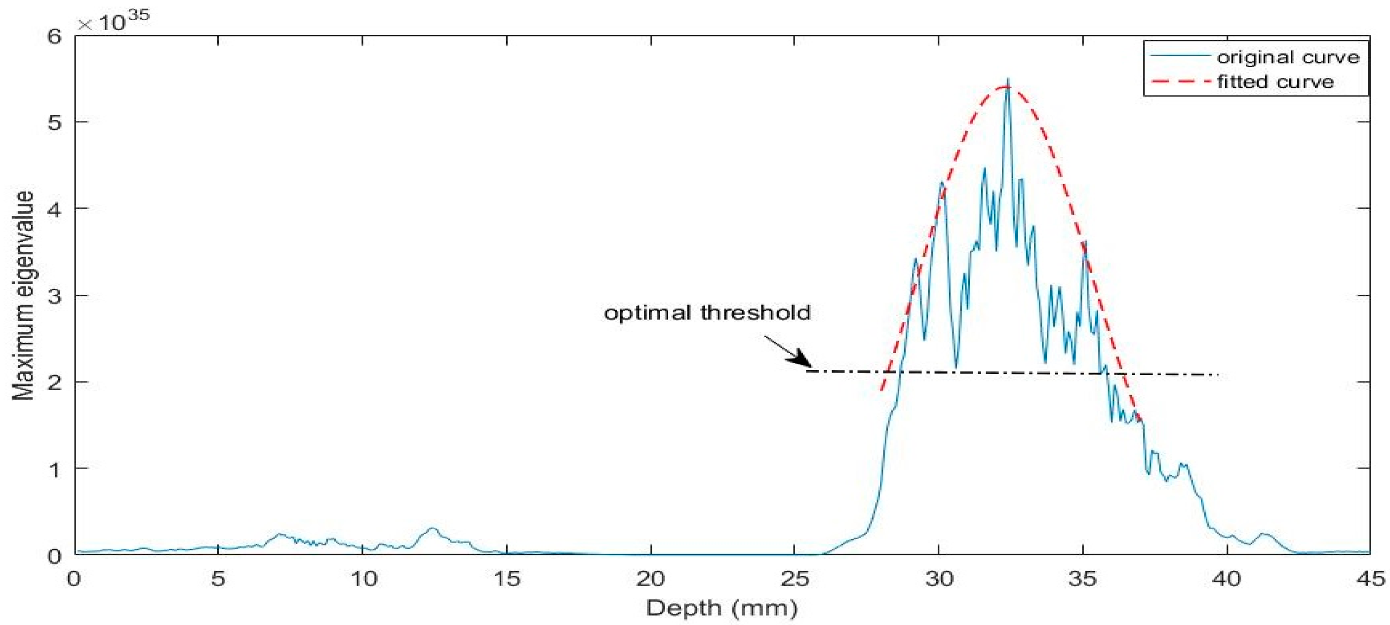
As is shown in Figure 3, the maximum eigenvalue curve of the UCA region is similar to a Gaussian function. The expression of the maximum eigenvalue curve can be represented as:
where x is the depth parameter; μ is the mean value; σ is the variance; and c is the amplitude. The eigenvalue of the UCA region can be set as [μ + e*σ, μ − e*σ], where e is an adjustable parameter.
Taking the area at the width of 10 mm as an example, the eigenvalue curve and the fitted curve is shown in Figure 5, where c = 5.4e35, μ = 32.3, σ = 4.2, and e is chosen as 1.
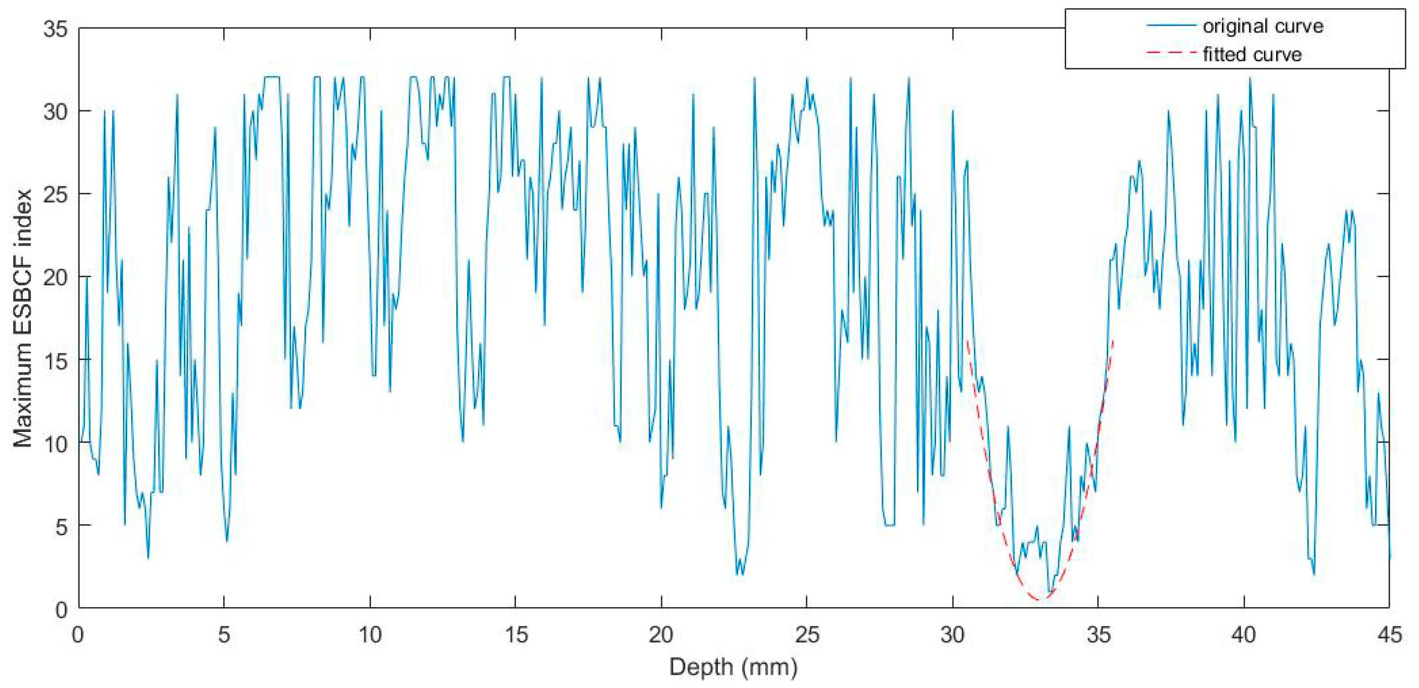
The ESBCF
Similarly, we fit the ESBCF curve by a Gaussian function. The ESBCF threshold can be set as [μ + e*σ, μ − e*σ], where e is an adjustable parameter. Taking the area at the width of 10 mm as an example, the eigenvalue curve and the fitted curve is shown in Figure 6.
3. Experiment and Results
3.1. Phantom Results
Two types of phantom experiments were designed. In the first, there were two wall-less pipes with different thicknesses in the phantom experiment (0.3 mm and 0.5 mm). In the other experiment, we placed a piece of fresh pork over the phantom, which only had one single pipe (about 0.5 mm). The detailed parameters for the phantom experiment are illustrated in Table 2.
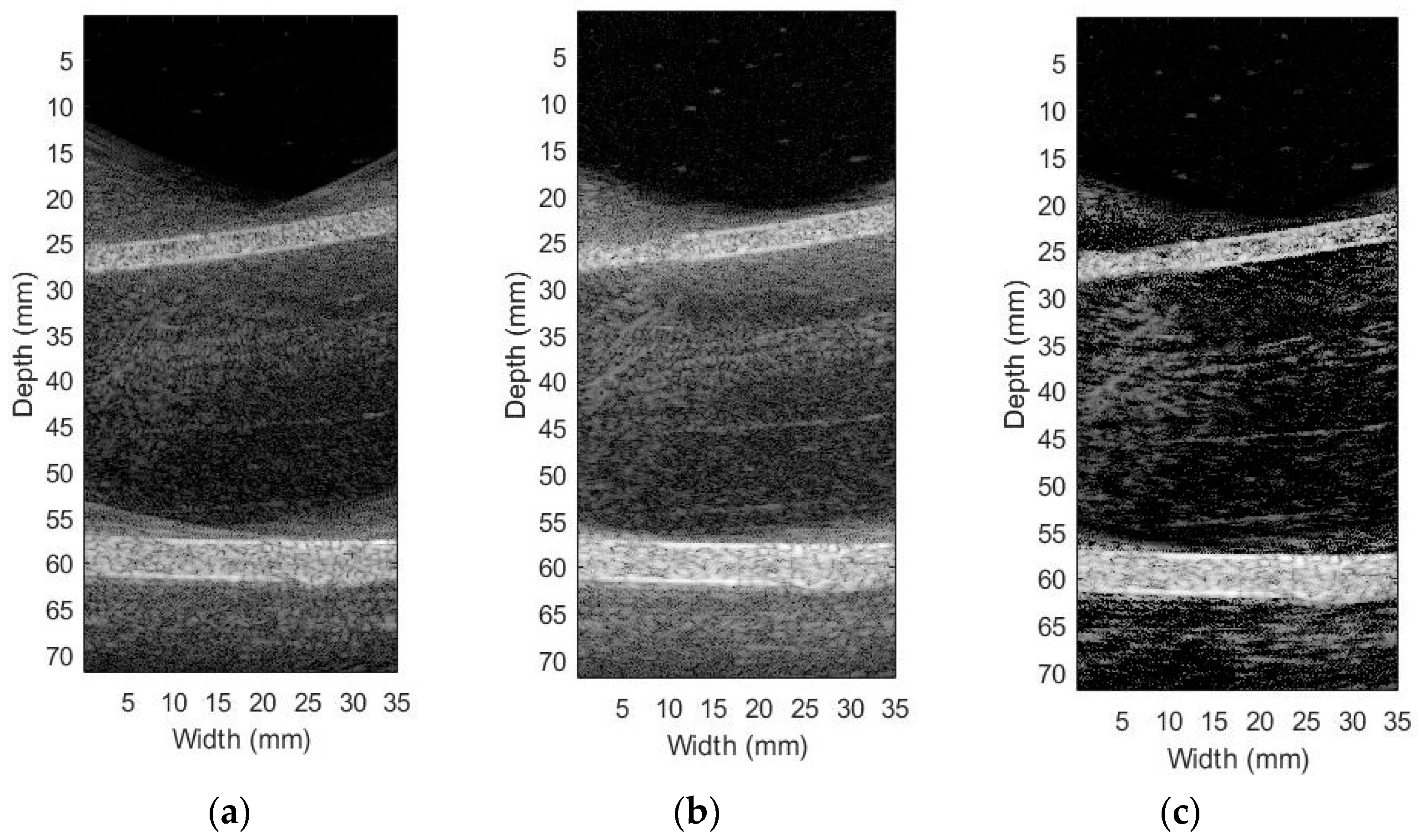
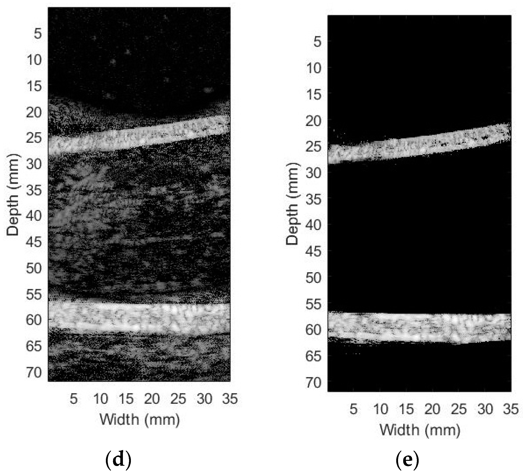
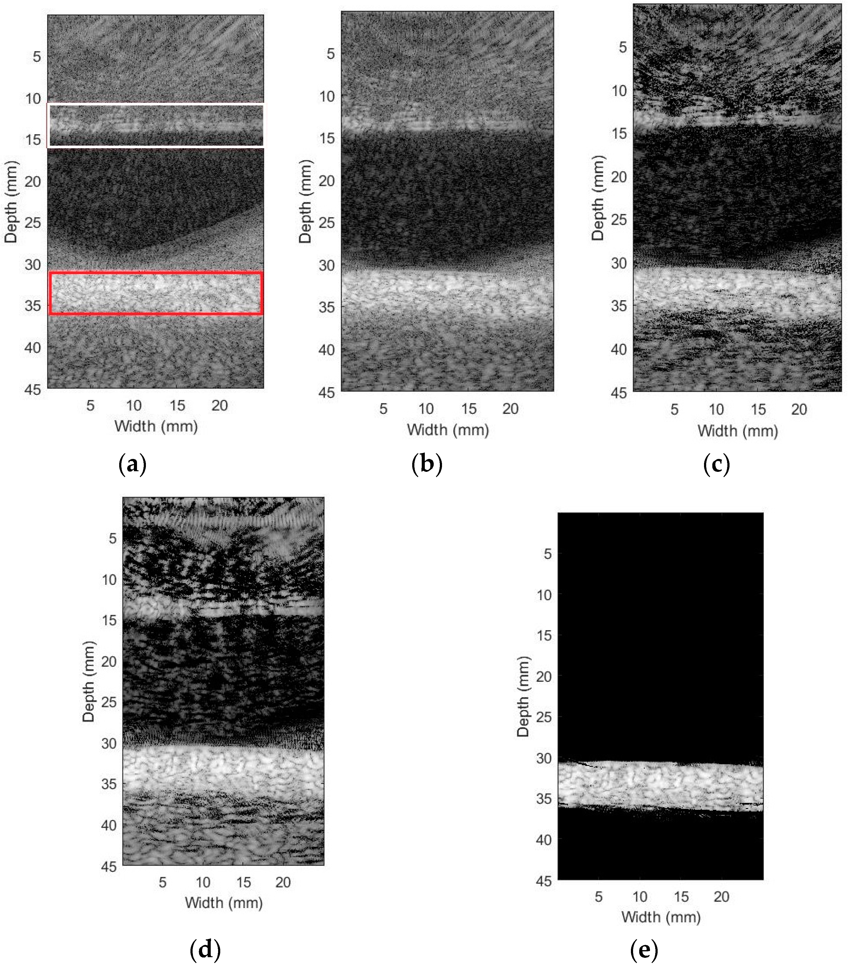
Figure 7 provides the first phantom result (transmit frequency: 3 MHz, transmit voltage: 10 V). Figure 7a–c show the imaging using traditional DAS, MV, and ESBMV beamformer without BWT, respectively. Figure 7d is the image using BWT based on ESBMV beamformer and Figure 7e is the image with bubble region detection by setting the maximum eigenvalue and ESBCF index threshold based on Figure 7d. Some impurities in the phantom are removed and the two tubes filled with microbubbles are well-preserved using the proposed method.
Figure 8 provides the pork experiment results. As shown in Figure 8, DAS suffers from severe artefact interference, althouth the artefact interference was weakened with MV. The image CR can be further improved with ESBMV, although an obvious black region distortion appears inside the tube. The brightness of the UCA inside the tube became more uniform and UCA information loss could be solved with the help of BWT, although the interference of tissues still exists. In comparison, for bubble region detection, the region except for the microbubble was able to be fully eliminated.
CTR was calculated to describe the performance of different beamformers:
where IUCA is the average intensity of the UCA region and Itissue is that of the tissue region. The two regions were enclosed in a rectangular area (the upper white one is the tissue region and the lower red one is the UCA region).
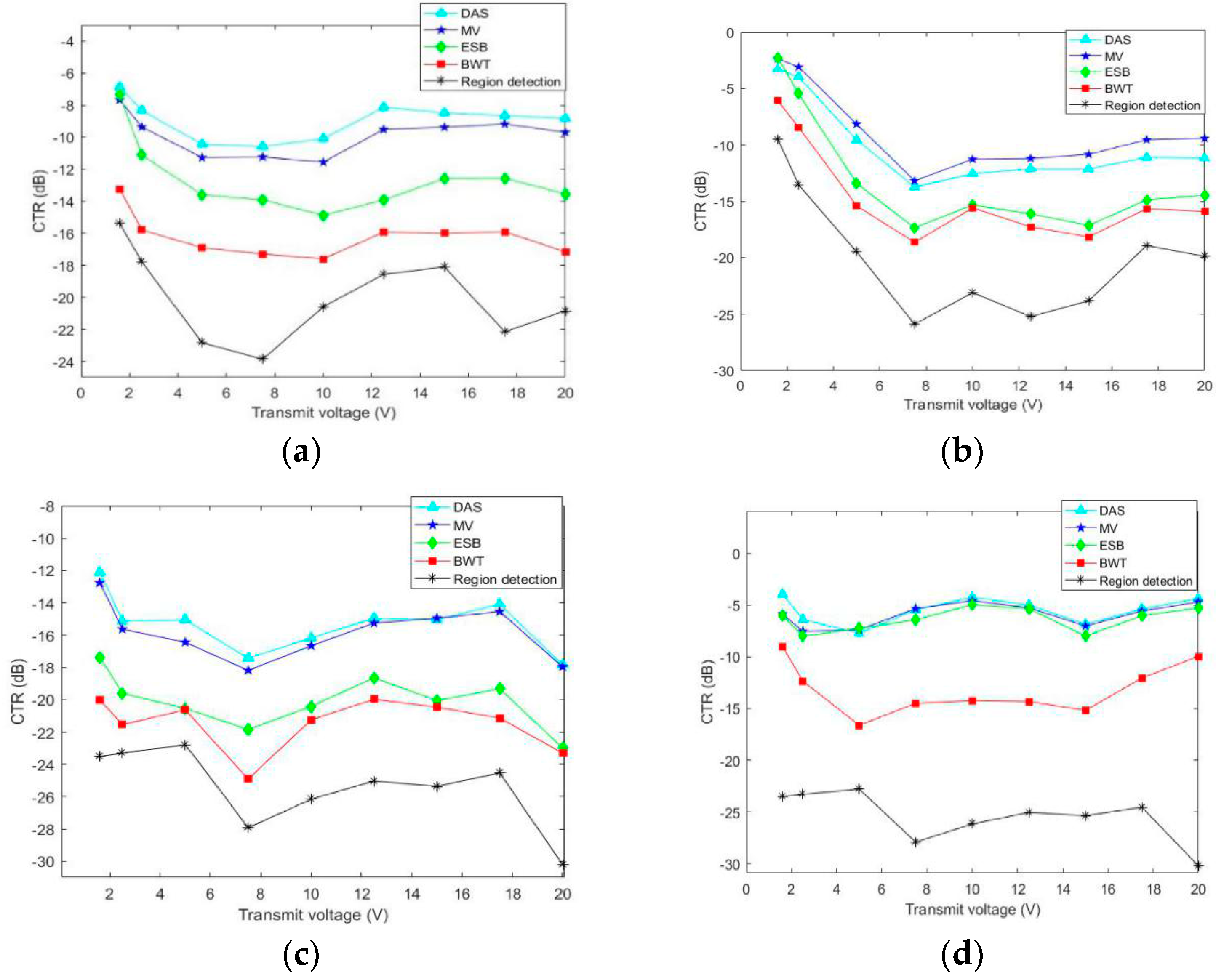
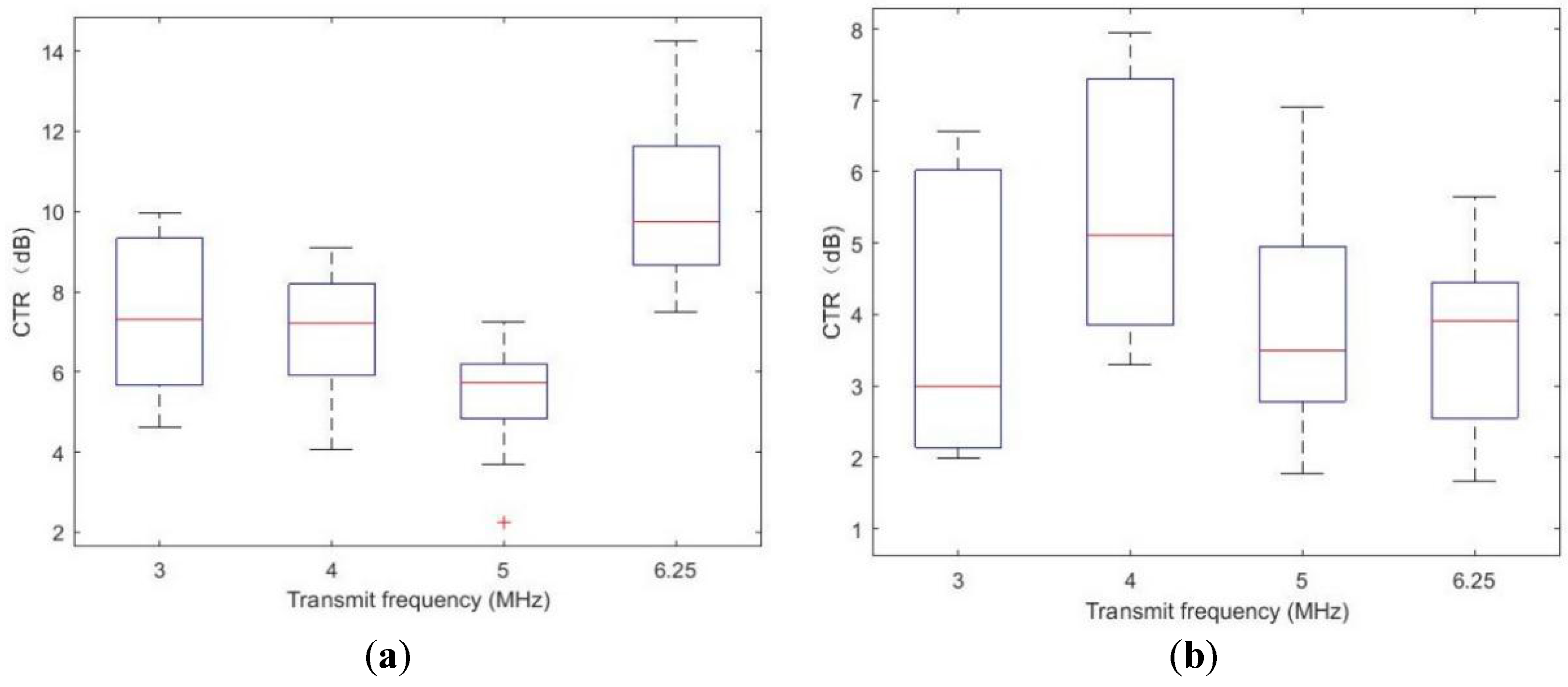
Figure 9 shows the CTR curve between different beamformers under different transmit conditions. The performance of bubble region detection was remarkable. Figure 10 explains that, with bubble region detection, the CTR has an enhancement of 7.5 dB on average compared with ESBMV, and an enhancement of 4.2 dB compared with BWT.
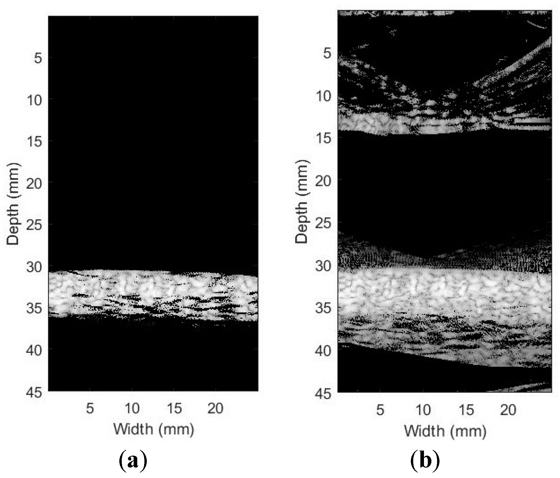
In the bubble region detection, the choice of eigenvalue and ESBCF index are two critical factors. Taking the pork experiment as an experiment, the pork and artifact disturbance remain under a low threshold while part of the UCA information is also removed with a high threshold, as shown in Figure 11.
3.2. In Vivo Results
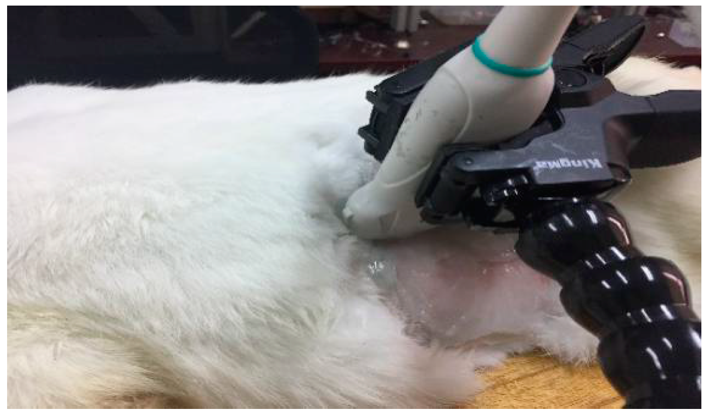
To demonstrate the effectiveness of the proposed algorithm, we also performed in vivo rabbit experiments. The ear vein and kidney of rabbit were studied, respectively. Figure 12 shows a scene from the rabbit experiment targeting the kidney.
The rabbit (2 kg, 4 months old) was first anesthetized and then placed on an autopsy table where the four limbs were fixed by ropes. Before imaging, the region of interest was epilated to remove the influence of cony hair. Medical ultrasonic coupling agent was applied to the region of interest. A total of 500 μL Sonovue microbubbles (no dilution) were injected through the right ear vein, which was followed by 500 μL of physiological saline.
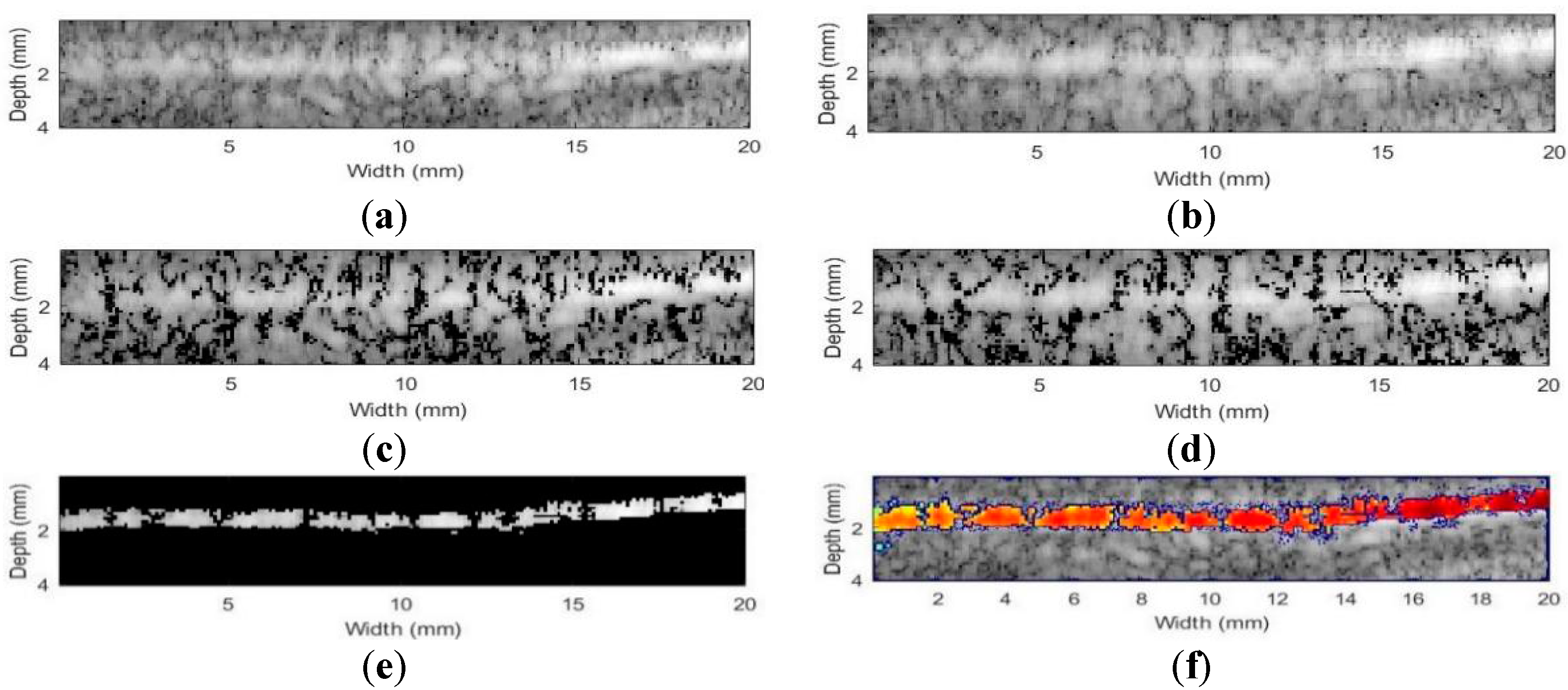
The image results after microbubble injection are shown below (3 MHz, 10 V), and we added the detected UCA region to the DAS image. Figure 13 is the image targeting the ear vein (c = 1) and Figure 14 is the kidney (c = 1).
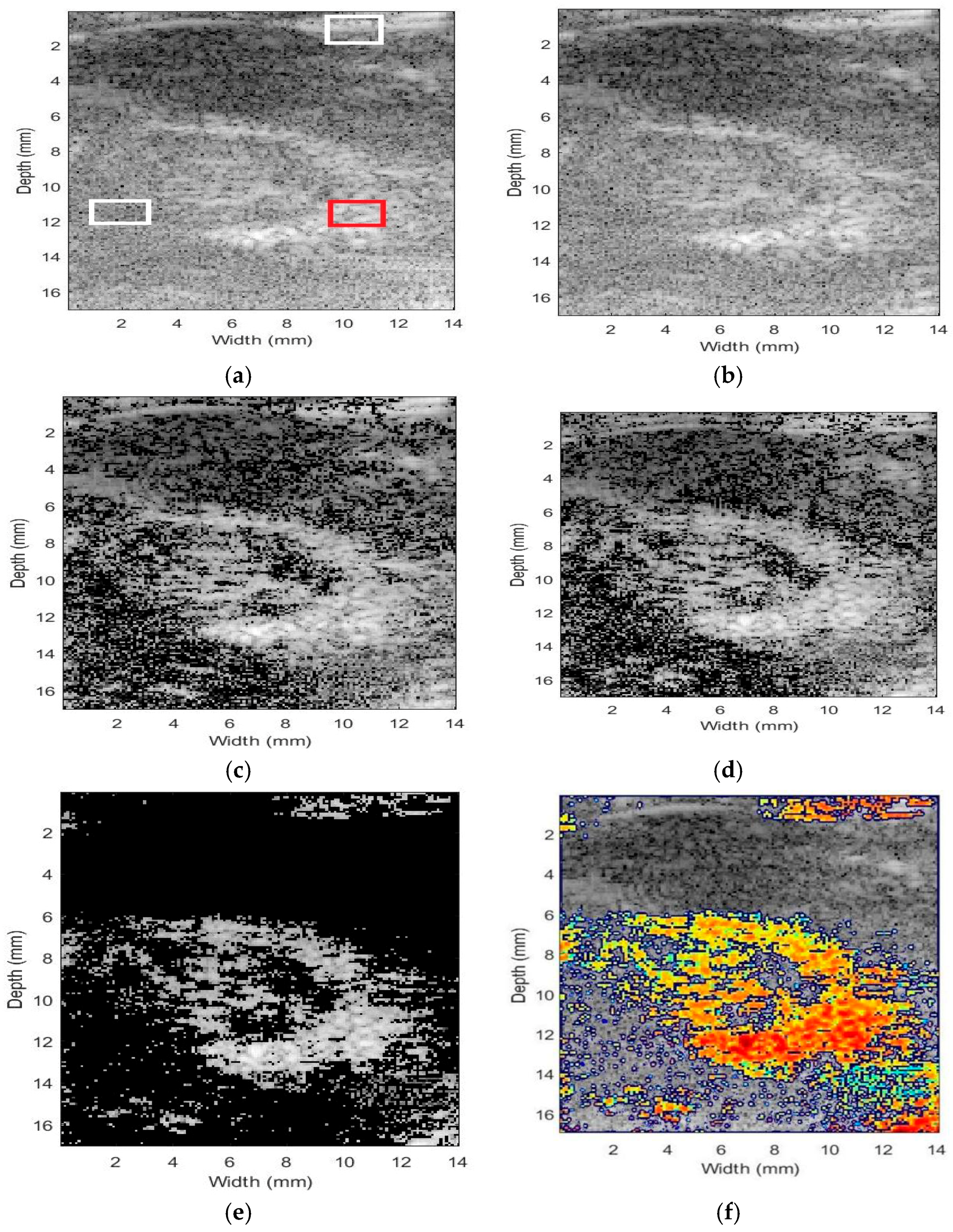
Bubble region detection can remove the noise around the kidney edge effectively, and makes the image clearer. However, the upper part of the muscle and part of the speckle noise in the image cannot be eradicated. This indicates that the tissue signal and the UCA signal still have partial overlap in terms of eigenvalues and ESBCF.
Taking the intensity in the red rectangle as the UCA and the white rectangles as the tissue region (CTR1 is calculated for the tissue and UCA regions with the same depth, while CTR2 is calculated with the same width, see Figure 14a), the CTR of different beamformers is shown in Table 3. CTR1 and CTR2 are improved by 18.0 dB and 18.0 dB compared with PWI based on DAS, while this improvement is 3.4 dB and 7.3 dB compared to imaging based on BWT.
4. Conclusions
The major purpose of USCAI is to enhance the contrast between microbubble perfusion regions and surrounding regions. In this paper, a new USCAI method based on bubble region detection was proposed. This method is used to maximize the role of USCAI by taking the dissimilarity of tissue and UCA in both frequency and spatial domains into account. BWT is used to highlight UCA information from the time-frequency domain. The UCA and tissue region is further detected by utilizing their differences with the combination of maximum eigenvalue and ESBCF index. Both phantom and in vivo rabbit experiments were designed to evaluate the performance of our proposed method. It is demonstrated that the bubble edge detection we proposed provides a significant enhancement in CTR, outperforming ESBMV and BWT. The phantom and in vivo experimental results show the potential of our method for filtering out the interfering components and retaining the information of microbubbles.
Acknowledgments
This work was supported by the National Basic Research Program of China (61471125).
Author Contributions
Y.H. and Y.T. designed and carried out the experimental studies and drafted the manuscript; J.Y., as a supervisor, revised the manuscript; J.Y., Y.W., Q.Z and L.C. discussed the method and results; and S.L. participated in the design of the experiment. All authors read and approved the final manuscript.
Conflicts of Interest
The authors declare no conflicts of interest.
References
- Cosgrove, D. Ultrasound contrast agents: An overview. Eur. J. Radiol. 2006, 60, 324–330. [Google Scholar] [CrossRef] [PubMed]
- Quaia, E. Microbubble ultrasound contrast agents: An update. Eur. Radiol. 2007, 17, 1995–2008. [Google Scholar] [CrossRef] [PubMed]
- Tang, M.X.; Kamiyama, N.; Eckersley, R.J. Effects of Nonlinear Propagation in Ultrasound Contrast Agent Imaging. Ultrasound Med. Biol. 2010, 36, 459–466. [Google Scholar] [CrossRef] [PubMed]
- Wilson, S.R.; Burns, P.N. Microbubble-enhanced US in body imaging: What role? Radiology 2010, 257, 24–39. [Google Scholar] [CrossRef] [PubMed]
- Blomley, M.J.K.; Cooke, J.C.; Unger, E.C.; Monaghan, M.J.; Cosgrove, D.O. Science, Medicine, and the Future: Microbubble Contrast Agents: A New Era in Ultrasound. BMJ Br. Med. J. 2001, 322, 1222–1225. [Google Scholar] [CrossRef]
- Couture, O.; Fink, M.; Tanter, M. Ultrasound contrast plane wave imaging. IEEE Trans. Ultrason. Ferroelectr. Freq. Control 2012, 59, 2676–2683. [Google Scholar] [CrossRef] [PubMed]
- Tremblaydarveau, C.; Williams, R.; Milot, L.; Bruce, M.; Burns, P.N. Combined perfusion and doppler imaging using plane-wave nonlinear detection and microbubble contrast agents. IEEE Trans. Ultrason. Ferroelectr. Freq. Control 2014, 61, 1988–2000. [Google Scholar] [CrossRef] [PubMed]
- Smeenge, M.; Mischi, M. Novel contrast-enhanced ultrasound imaging in prostate cancer. World J. Urol. 2011, 29, 581–587. [Google Scholar] [CrossRef] [PubMed]
- Wilkening, W.; Krueger, M.; Ermert, H. Phase-coded pulse sequence for non-linear imaging. In Proceedings of the IEEE Ultrasonics Symposium (IUS), San Juan, Puerto Rico, 22–25 October 2000. [Google Scholar]
- Wang, D.; Xuan, Y.; Wan, J.; Jing, B.; Lei, Z.; Wan, M. Ultrasound contrast plane wave imaging with higher CTR based on pulse inversion bubble wavelet transform. In Proceedings of the IEEE International Ultrasonics Symposium Ius (IUS), Chicago, IL, USA, 3–6 September 2014; pp. 1762–1765. [Google Scholar]
- Wang, D.; Zong, Y.; Yang, X.; Hu, H.; Wan, J.; Zhang, L.; Bouakaz, A.; Wan, M. Ultrasound contrast plane wave imaging based on bubble wavelet transform: In vitro and in vivo validations. Ultrasound Med. Biol. 2016, 42, 1584–1597. [Google Scholar] [CrossRef] [PubMed]
- Burns, P.N.; Wilson, S.R.; Simpson, D.H. Pulse inversion imaging of liver blood flow: Improved method for characterizing focal masses with microbubble contrast. Investig. Radiol. 2010, 35, 58–71. [Google Scholar] [CrossRef]
- Eckersley, R.J.; Chin, C.T.; Burns, P.N. Optimising phase and amplitude modulation schemes for imaging microbubble contrast agents at low acoustic power. Ultrasound Med. Biol. 2005, 31, 213–219. [Google Scholar] [CrossRef] [PubMed]
- Shen, C.C.; Lin, C.H. Chirp-encoded excitation for dual-frequency ultrasound tissue harmonic imaging. IEEE Trans. Ultrason. Ferroelectr. Freq. Control 2012, 59, 2420–2430. [Google Scholar] [PubMed]
- Shen, C.C.; Shi, T.Y. Golay-encoded excitation for dual-frequency harmonic detection of ultrasonic contrast agents. IEEE Trans. Ultrason. Ferroelectr. Freq. Control 2011, 58, 349–356. [Google Scholar] [CrossRef] [PubMed]
- Shekhar, H.; Doyley, M.M. The response of phospholipid-encapsulated microbubbles to chirp-coded excitation: Implications for high-frequency nonlinear imaging. J. Acoust. Soc. Am. 2013, 133, 3145–3158. [Google Scholar] [CrossRef] [PubMed]
- Doinikov, A.A.; Bouakaz, A. Review of shell models for contrast agent microbubbles. IEEE Trans. Ultrason. Ferroelectr. Freq. Control 2011, 58, 981–993. [Google Scholar] [CrossRef] [PubMed]
- Lu, S.; Xu, S.; Liu, R.; Hu, H.; Wan, M. High-contrast active cavitation imaging technique based on multiple bubble wavelet transform. J. Acoust. Soc. Am. 2016, 140, 1000–1011. [Google Scholar] [CrossRef] [PubMed]
- Liu, R.; Xu, S.; Hu, H.; Huo, R.; Wang, S.; Wan, M. Wavelet-transform-based active imaging of cavitation bubbles in tissues induced by high intensity focused ultrasound. J. Acoust. Soc. Am. 2016, 140, 798–805. [Google Scholar] [CrossRef] [PubMed]
- Doinikov, A.A.; Haac, J.F.; Dayton, P.A. Modeling of nonlinear viscous stress in encapsulating shells of lipid-coated contrast agent microbubbles. Ultrasonics 2009, 49, 269–275. [Google Scholar] [CrossRef] [PubMed]
- Sijl, J.; Overvelde, M.; Dollet, B.; Garbin, V.; de Jong, N.; Lohse, D.; Versluis, M. “Compression-only” behavior: A second-order nonlinear response of ultrasound contrast agent microbubbles. J. Acoust. Soc. Am. 2011, 129, 1729–1739. [Google Scholar] [CrossRef] [PubMed]
- Faez, T.; Emmer, M.; Kooiman, K.; Versluis, M.; van der Steen, A.F.; de Jong, N. 20 years of ultrasound contrast agent modeling. IEEE Trans. Ultrason. Ferroelectr. Freq. Control 2013, 60, 7–20. [Google Scholar] [CrossRef] [PubMed]
- Capon, J. High-resolution frequency-wavenumber spectrum analysis. Proc. IEEE 2005, 57, 1408–1418. [Google Scholar] [CrossRef]
- Asl, B.M.; Mahloojifar, A. Eigenspace-based minimum variance beamforming applied to medical ultrasound imaging. IEEE Trans. Ultrason. Ferroelectr. Freq. Control 2010, 57, 2381–2390. [Google Scholar] [CrossRef] [PubMed]
- Johnstone, I.M. On the Distribution of the Largest Eigenvalue in Principal Components Analysis. Ann. Stat. 2001, 29, 295–327. [Google Scholar] [CrossRef]
- Zeng, Y.; Liang, Y.C. Eigenvalue based Spectrum Sensing Algorithms for Cognitive Radio. IEEE Trans. Commun. 2008, 57, 1784–1793. [Google Scholar] [CrossRef]
- Kortun, A.; Ratnarajah, T.; Sellathurai, M.; Liang, Y.C.; Zeng, Y. Throughput analysis using eigenvalue based spectrum sensing under noise uncertainty. In Proceedings of the Wireless Communications and Mobile Computing Conference, Limassol, Cyprus, 27–31 August 2012; pp. 395–400. [Google Scholar]
- Zeng, Y.; Liang, Y.C.; Peh, E.C.Y.; Hoang, A.T. Cooperative covariance and eigenvalue based detections for robust sensing. In Proceedings of the Global Telecommunications Conference (GLOBECOM 2009), Honolulu, HI, USA, 30 November–4 December 2009; pp. 1–6. [Google Scholar]
- Hollman, K.W.; Rigby, K.W.; O’Donnell, M. Coherence factor of speckle from a multi-row probe. Proc. IEEE 1999, 2, 1257–1260. [Google Scholar]
- Xu, M.; Yang, X.; Ding, M.; Yuchi, M. Spatio-temporally smoothed coherence factor for ultrasound imaging. IEEE Trans. Ultrason. Ferroelectr. Freq. Control 2014, 61, 182–190. [Google Scholar] [CrossRef] [PubMed]
- Wei, G.; Wang, Y.; Yu, J. Ultrasound harmonic enhanced imaging using eigenspace-based coherence factor. Ultrasonics 2016, 72, 106–116. [Google Scholar]
Figure 1.
The phantom experiment setup (with pork).

Figure 2.
The image of the phantom (with pork) under delay-and-sum (DAS).

Figure 3.
The maximum eigenvalue curve of different depths.

Figure 4.
The maximum eigenspace-based coherence factor (ESBCF) value index curve of different depths.
Figure 4.
The maximum eigenspace-based coherence factor (ESBCF) value index curve of different depths.

Figure 5.
The fitted eigenvalue curve.

Figure 6.
The fitted maximum ESBCF index curve.

Figure 7.
The image results of the phantom experiment (without pork): (a) DAS; (b) minimum variance (MV); (c) Eigenspace-based minimum variance (ESBMV); (d) BWT; (e) bubble region detection (dynamic range is 60 dB).
Figure 7.
The image results of the phantom experiment (without pork): (a) DAS; (b) minimum variance (MV); (c) Eigenspace-based minimum variance (ESBMV); (d) BWT; (e) bubble region detection (dynamic range is 60 dB).


Figure 8.
The image results of phantom experiment (with pork): (a) DAS; (b) MV; (c) ESBMV; (d) BWT; (e) bubble region detection.
Figure 8.
The image results of phantom experiment (with pork): (a) DAS; (b) MV; (c) ESBMV; (d) BWT; (e) bubble region detection.

Figure 9.
The image contrast-to-tissue ratio (CTR) curve between different beamformers: (a) 3 MHz; (b) 4 MHz; (c) 5 MHz; and (d) 6.25 MHz.
Figure 9.
The image contrast-to-tissue ratio (CTR) curve between different beamformers: (a) 3 MHz; (b) 4 MHz; (c) 5 MHz; and (d) 6.25 MHz.

Figure 10.
Increase in CTR with bubble region detection: (a) Increase in CTR between region detection and ESBMV; and (b) increase in CTR between region detection and BWT.
Figure 10.
Increase in CTR with bubble region detection: (a) Increase in CTR between region detection and ESBMV; and (b) increase in CTR between region detection and BWT.

Figure 11.
The image result of bubble region detection under different thresholds: (a) Higher threshold and (b) lower threshold.
Figure 11.
The image result of bubble region detection under different thresholds: (a) Higher threshold and (b) lower threshold.

Figure 12.
The in vivo rabbit experiment targeting the kidney.

Figure 13.
The image result of ear vein: (a) DAS; (b) MV; (c) ESBMV; (d) BWT; (e) bubble region detection; and (f) UCA-enhanced image.
Figure 13.
The image result of ear vein: (a) DAS; (b) MV; (c) ESBMV; (d) BWT; (e) bubble region detection; and (f) UCA-enhanced image.

Figure 14.
The image result of kidney: (a) DAS; (b) MV; (c) ESBMV; (d) BWT; (e) bubble region detection; and (f) UCA -enhanced image.
Figure 14.
The image result of kidney: (a) DAS; (b) MV; (c) ESBMV; (d) BWT; (e) bubble region detection; and (f) UCA -enhanced image.


Table 1.
The central frequency of the bubble wavelet with different transmit frequencies and their optimal scale factors.
Table 1.
The central frequency of the bubble wavelet with different transmit frequencies and their optimal scale factors.
| Transmit Frequency (MHz) | Central Frequency of Wavelet (Fc) | Optimal Scale Factor (a) | Central Frequency after Bubble Wavelet Transformation (BWT) (F(a); in MHz) |
|---|---|---|---|
| 3 | 0.9394 | 0.16 | 5.87 |
| 4 | 0.6133 | 0.07 | 8.76 |
| 5 | 0.7869 | 0.08 | 9.83 |
| 6.25 | 0.8750 | 0.07 | 12.5 |
Table 2.
Parameters for the experiment.
| Experiment Parameters | Value |
|---|---|
| Transducer element number | 128 |
| Transducer element kerf | 0.05 mm |
| Transducer element width | 0.27 mm |
| Transducer element pitch | 0.3 mm |
| Transducer spacing between elements | 0. 295 mm |
| Transmit frequency | 3 MHz, 4 MHz, 5 MHz, 6.25 MHz |
| Transmit voltage | 1.6 V, 2.5 V, 5 V, 7.5 V, 10 V, 12.5 V, 15 V, 17.5 V, 20 V |
| Transmit pulse | Sine wave with two cycles |
Table 3.
The image CTR of different beamformers.
| Beamformer | CTR1 (dB) | CTR2 (dB) |
|---|---|---|
| DAS | −10.1 | −4.9 |
| MV | −10.3 | −5.2 |
| ESBMV | −20.6 | −12.6 |
| BWT | −24.7 | −15.6 |
| Bubble region detection | −28.1 | −22.9 |
© 2017 by the authors. Licensee MDPI, Basel, Switzerland. This article is an open access article distributed under the terms and conditions of the Creative Commons Attribution (CC BY) license (http://creativecommons.org/licenses/by/4.0/).
Share and Cite
MDPI and ACS Style
Huang, Y.; Yu, J.; Tong, Y.; Li, S.; Chen, L.; Wang, Y.; Zhang, Q. Contrast-Enhanced Ultrasound Imaging Based on Bubble Region Detection. Appl. Sci. 2017, 7, 1098. https://doi.org/10.3390/app7101098
AMA Style
Huang Y, Yu J, Tong Y, Li S, Chen L, Wang Y, Zhang Q. Contrast-Enhanced Ultrasound Imaging Based on Bubble Region Detection. Applied Sciences. 2017; 7(10):1098. https://doi.org/10.3390/app7101098
Chicago/Turabian StyleHuang, Yurong, Jinhua Yu, Yusheng Tong, Shuying Li, Liang Chen, Yuanyuan Wang, and Qi Zhang. 2017. "Contrast-Enhanced Ultrasound Imaging Based on Bubble Region Detection" Applied Sciences 7, no. 10: 1098. https://doi.org/10.3390/app7101098
Note that from the first issue of 2016, this journal uses article numbers instead of page numbers. See further details here.