A Precise Positioning Method for a Puncture Robot Based on a PSO-Optimized BP Neural Network Algorithm

1
The Department of Automation, University of Science and Technology of China, Hefei 230026, China
2
Key Laboratory of Special Robot Technology of Jiangsu Province, Hohai University, Changzhou 213000, China
3
School of Information Engineering, Southwest University of Science and Technology, Mianyang 621010, China
4
Institute of Intelligent Manufacturing Technology, Jiangsu Industrial Technology Research Institute, Nanjing 211800, China
*
Authors to whom correspondence should be addressed.
Appl. Sci. 2017, 7(10), 969; https://doi.org/10.3390/app7100969
Submission received: 18 July 2017
/
Revised: 12 September 2017
/
Accepted: 18 September 2017
/
Published: 21 September 2017
(This article belongs to the Special Issue Bio-Inspired Robotics)
Abstract
:The problem of inverse kinematics is fundamental in robot control. Many traditional inverse kinematics solutions, such as geometry, iteration, and algebraic methods, are inadequate in high-speed solutions and accurate positioning. In recent years, the problem of robot inverse kinematics based on neural networks has received extensive attention, but its precision control is convenient and needs to be improved. This paper studies a particle swarm optimization (PSO) back propagation (BP) neural network algorithm to solve the inverse kinematics problem of a UR3 robot based on six degrees of freedom, overcoming some disadvantages of BP neural networks. The BP neural network improves the convergence precision, convergence speed, and generalization ability. The results show that the position error is solved by the research method with respect to the UR3 robot inverse kinematics with the joint angle less than 0.1 degrees and the output end tool less than 0.1 mm, achieving the required positioning for medical puncture surgery, which demands precise positioning of the robot to less than 1 mm. Aiming at the precise application of the puncturing robot, the preliminary experiment has been conducted and the preliminary results have been obtained, which lays the foundation for the popularization of the robot in the medical field.
1. Introduction
Robots are currently used in industrial and medical applications where high accuracy, repeatability, and stability of the operations are required [1]. With the development of modern control technology, robot technology has been widely used in new fields, such as in medical robots. A surgical robot operating system is a collection of a number of modern, complex, high technologies, and the doctor, through the robot system, can perform surgical operations without touching patients. A minimally-invasive surgical robot is a combination of medical image processing technology and the operation of the mechanical arm to perform puncture surgery on the patient, to achieve minimal invasiveness, accuracy, efficiency, and stability.
The most important problem of the serial robot, which is the solution of the kinematics of the manipulator, can be successfully implemented. Robot kinematics handles the mapping between joint space (h) and Cartesian space (x, y, z), where h represents the positions of the joints of a robotic manipulator and (x, y, z) represent the position of the end effector of the manipulator [2]. Kinematics analysis of the robot includes two aspects: the forward kinematics and the inverse kinematics. The forward kinematics are the mappings from the joint angle to the Cartesian coordinate system. The inverse kinematics are known to solve the joint variables under the position and posture of the end effector.
Traditionally, there are three methods to solve the inverse kinematics problem of the robot: the geometric method, the algebraic method, and the iterative method. Any method has its own shortcomings in solving the inverse kinematics. For instance, closed-form solutions are not guaranteed for the algebraic methods, and closed-form solutions for the first three joints of the robot must exist geometrically when the geometric method is used. Similarly, the iterative inverse kinematics solution method converges to only one solution that depends on the starting point [1]. These methods often require high-performance computer hardware, and the calculation accuracy cannot be guaranteed. For these reasons, researchers have begun to focus on the application of artificial neural networks to the kinematics of the robot.
The inverse kinematics analysis of the six degrees of freedom (DOF) industrial robot is carried out by using the back propagation neural network algorithm [3], but this method cannot solve the problem when the joint angle error is too large. In [4], a method is presented for solving the inverse kinematics of redundant robots and the prevention of singular points. In [5], for the singular series robot arm configuration and uncertainty, a method was proposed based on an artificial neural network, and the training process is very difficult, and needs sensors added to each joint.
There are many researchers focusing on the genetic algorithm to obtain the inverse kinematics of the robot [6,7,8]. Kamal and Djamel [6] researched particle swarm optimization (PSO) and genetic algorithms (GA) for finite impulse response (FIR) filter design. Kalra and colleagues [7] used an evolutionary approach based on a real-coded genetic algorithm to obtain the multimodal inverse kinematics problem of industrial robots. In their method, the fitness function is defined in a manner that requires separate evaluation of the positional error of the robot and the total joint displacement. These two approaches can be used together to solve some specific problems. Mustafa and Kerim [8] used four different optimization algorithms (the genetic algorithm (GA), the particle swarm optimization (PSO) algorithm, the quantum particle swarm optimization (QPSO) algorithm, and the gravitational search algorithm (GSA)) for solving the inverse kinematics problem of a four DOF serial robot manipulator.
The main purpose of this paper is to improve the precision of the inverse kinematics solution from a particle swarm optimization (PSO) back propagation (BP) neural network algorithm, especially for processing data in a short period of time, and the time in which the robot is in motion. The particle swarm optimization algorithm is employed to find the global advantage with the BP neural network to find the optimal solution, overcome some inherent defects (easy to fall into local minimum, slow convergence and poor generalization ability etc.) of the BP neural network, and thus further improve the convergence precision of BP neural network, the convergence speed, and generalization ability. The main contribution is that the algorithm is applied to the inverse kinematics of UR six degree of freedom manipulator, which guarantees the accuracy of the end position accuracy of the robot with six degrees of freedom within 0.1 mm, and the robot joint angle at 0.01 degrees. The main innovation of this study is the application of this technique in the precise localization of medical needle surgery. In the experimental part, we achieved very good results and achieved high-precision positioning of the puncture operation. We had to ensure that the experimental puncture accuracy was less than 1 mm, which can meet the needs of medical needle surgery.
2. Research and Methods
2.1. The Principle of Precision Positioning of a Puncture Robot
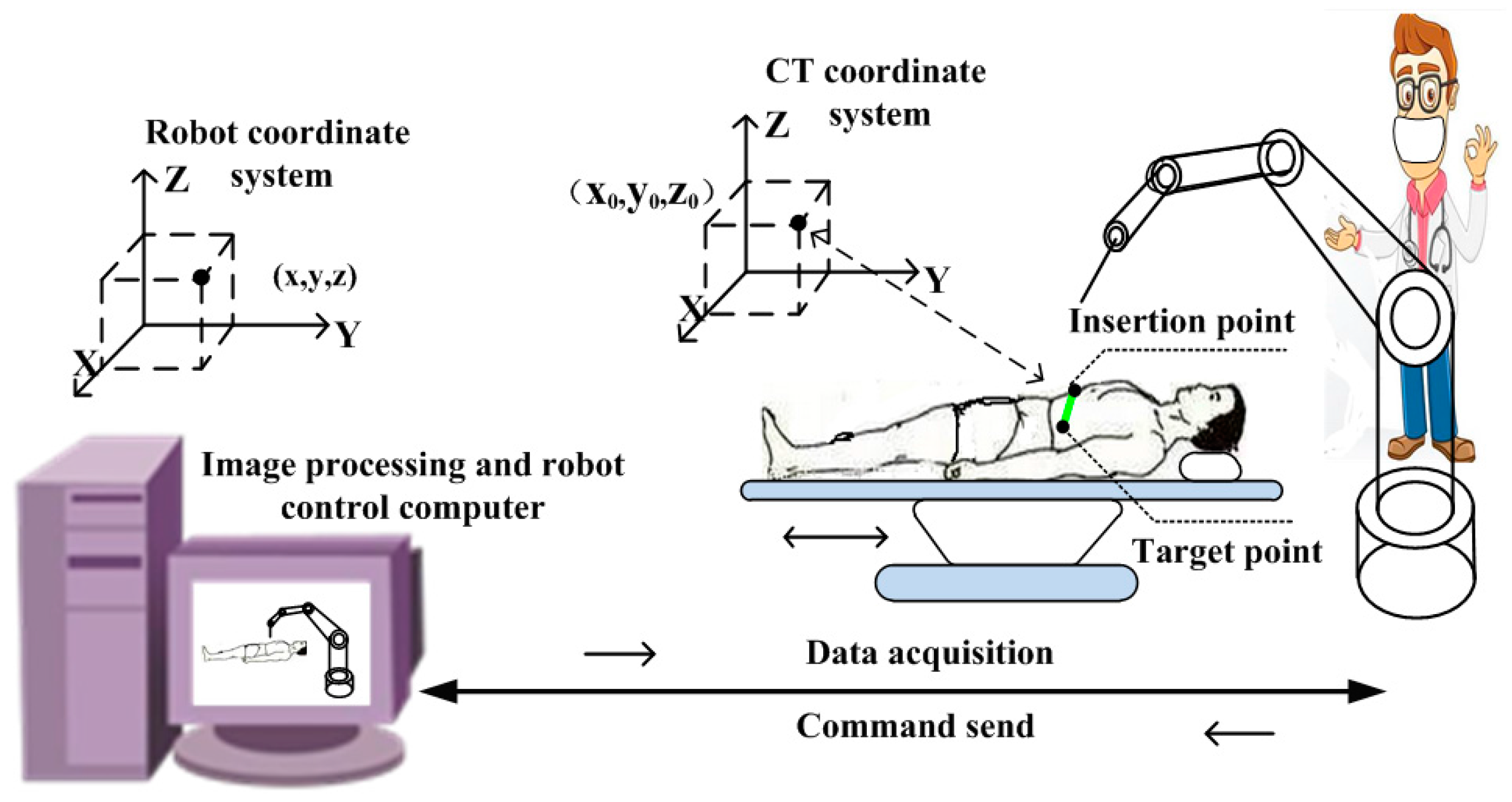
Minimally-invasive surgery (MIS) is a cost-effective alternative to open surgery whereby essentially the same operations are performed using specialized instruments designed to fit into the body through several tiny punctures instead of one large incision [9]. The principle of the operation of the puncture robot is shown in Figure 1.
Firstly, patients require a CT scan, and the medical image will be generated by the computer to complete the three-dimensional reconstruction. Then a doctor can observe and diagnose the disease according to the three-dimensional model. Finally, the doctor determines the position of the puncture target point coordinates, and determines the insertion point through the analysis of the patients’ skin. Between the target point and insertion point of connection is the puncture route (the green line in Figure 1). The route must avoid the patient’s bones, blood vessels, and other organs. The accurate puncture route directly determines the quality of the puncturing operation. Research on precise positioning technology of the manipulator used in this study was conducted to establish the series robot puncture route. The puncture route target point and insertion point coordinates are sent to the robot through the data processing computer, and at the end-effector of the robot, the puncture guide tube accurately positions the needle into the patient’s skin, the puncture route keeping with the robot end position and posture.
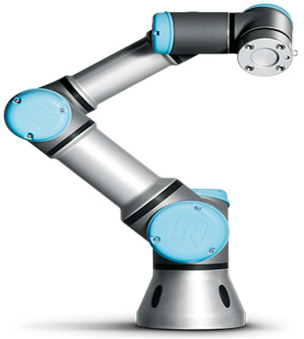
2.2. Analysis of the UR3 Manipulator
The UR3 manipulator (Figure 2) is a new and small six DOF collaborative robotic by the Universal Robots Company (Odense, Denmark). The key features of the UR3 manipulator are that it is a flexible, lightweight, collaborative, and safe table-top robot. The UR3’s six joints contribute to the transformational and rotational movements of its end effector. The kinematics analysis of the UR3 is more complex than other manipulators. The Schematic and frame assignment of UR3 is shown in Figure 3.
Currently, there are no exact Matlab models for this robot. In this paper, we researched the precise positioning technique using the UR3 for medical puncture surgery. Kinematic modeling of the robot based on the Denavit-Hartenberg (D-H) parameters provided by the UR3 manual are shown in Table 1.
The robot homogeneous transformation matrix for a single joint is expressed in Equations (1) and (2), which uses four link parameters [10]. This transformation is known as the D-H notation:
based on the transformation matrix between adjacent links . Among them, depend on the constant of robot structure parameters; represent the joint variables, , and . Thus, we can obtain the transformation matrix from the base to the end effector, whose position matrix by the homogeneous coordinate transformation is given by Equation (3):
Among them, is the rotation matrix of the robot end effector, and is the position matrix of the robot end effector, where represents the rotational elements of the transformation matrix (i and j = 1, 2, 3) and are the elements of the position vector.
A UR3 robot with six DOF was used in this study. The manipulator has a six DOF Cartesian position of the end effector (x, y, z), which is obtained directly from the matrix [11]. The orientation of the end effector is described according to the RPY (roll-pitch-yaw) rotation. These rotations are the angles around the Z-Y-Z axis, as shown in Equation (4):
Solving the matrix, we can obtain the angles, which are calculated by Equations (5)–(7):
These equations can provide the robot position, which is relative to the universe coordinate system [12]. The coordinates of each joint are used to describe the position and orientation of the robot. The forward kinematics equation of the robot is described by Equation (8):
As shown in Equation (8), when the six joint angles of the robot are known, the Cartesian coordinate system of the robot can be calculated according to the forward kinematics [13]. However, the six joint angles of the robot must be computed in an industrial application, so the inverse kinematics equation is solved by Equation (9):
In the next part, will be used as the input variables of the BP neural network model, and the joint angles will be used as the output variables of the BP neural network.
2.3. BP Neural Network
A BP (back propagation) network, which was proposed by Rumelhart and McCelland in 1986, is a type of error back propagation training algorithm for the multilayer feedforward network. It consists of two processes: the forward spread of information and the reverse propagation of error; the neural network model is one of the most widely used. BP neural networks can be compared to the input and output of the highly nonlinear mapping, which is characterized by the spread of the error to correct the weights and thresholds of the network. By approximating the nonlinear function several times, the BP neural network can approximate the complex function. A BP neural network model of a single neuron is shown in Figure 4.
For a given artificial neuron, is the component of the input vector of the neuron, is the weight component of the input vector of the neuron, and represents a threshold or bias. Usually, the x0 input is assigned the value −1, which makes it a bias input with wk0 = θ. This leaves only actual inputs to the neuron: from x1 to xn.
The output of the yi neuron is expressed in Equation (10):
where f is the transfer function. We approximate the function by the sigmoid function. If the weight is positive, it means that the corresponding input point is in a state of excitement and has a strengthening effect; if the weight is negative, it has an inhibiting effect. The function is expressed in Equation (11):
In this paper, according to the network structure, the input layer has six neurons, respectively, corresponding to . The output layer has six neurons: the six joint angles corresponding to the UR3 robot’s six angles . The number of hidden layer units is a very complicated problem: its determination needs to agree with the experience of the designer and several tests. The hidden layer unit number with the number of input/output units has a direct relationship; if the number is too great, not only will the training time increase, causing the learning time to become too long, but the error may be large. If the number is too low, then the neural network may have too little information to solve the problem. Therefore, it is very important to select a suitable number of hidden layers [14,15]. In this paper, after a large number of comparisons and experiments, two hidden layers are selected: 24 and 18 units, respectively. In this paper, the design of the BP neural network topology is shown in Figure 5.
Figure 5 illustrates the topology of the designed network which consists of three layers, one of which is a hidden layer, presented to store the internal representation. The fundamental idea underlying the design of the network is that the information entering the input layer is mapped as an internal representation in the units of the hidden layer (s) and the outputs are generated by this internal representation, rather than by the input vector. Given that there are enough hidden neurons, input vectors can always be encoded in such a form that the appropriate output vector can be generated from any input vector [16].
Although BP neural networks have many remarkable characteristics, they also have some inherent defects: easily falling into a local minimum, slow convergence speed, and weak generalization ability. Therefore, they require some improvement by combining with an optimization algorithm.
2.4. PSO Optimization Combined with the BP Neural Network
Particle swarm optimization (PSO) was proposed by Kennedy and Eberhart [17], and is derived from the study of the behavior of bird predation combined with the regularity of the collective activity of birds to establish a simplified model by the population. The PSO algorithm also belongs to the area of evolutionary algorithms (EAs).
PSO, which is similar to a genetic algorithm, is an iterative optimization algorithm [18,19]. The system is initialized with a set of random solutions. PSO does not have a genetic algorithm “crossover” and “mutation” operation, rather, it follows the current search to find the optimal value of the global optimum. The PSO algorithm was brought to the attention of academic circles as it has the advantages of easy implementation, high precision, fast convergence, easy adjustment parameters, and so on. PSO has been extensively used in function optimization, neural network training, fuzzy control systems, and genetic algorithms.
Particle swarm optimization (PSO) is a parallel algorithm, and finds the optimal solution by iteration. In each iteration, the particle updates itself by tracking two extremes [20]. The first extreme is the optimal solution of the particle itself, called the personal best value (pbest); the other is the group best value (gbest). The target value is set as the best value of the fitness function, and i particles can be expressed as a D-dimensional vector , and the velocity of particles can be expressed as . The current best position of the particle is represented as , and the current optimal position of the individual is represented by . The best position of the particle group is represented as , , representing the historical optimal location of a group. In each iteration, the particle swarm updates its speed and position by the individual extreme value, and the group extreme value. The updated formula is shown in Equations (12) and (13):
where and are, respectively, the position and velocity of the i-th particle at the k-th iteration. V is the velocity of the particle, is the weighting function, r1 and r2 are random numbers between 0 and 1, and c1 and c2 are learning factors; usually, c1 = c2 = 2. is the deviation of the individual extreme value, and is the deviation of the group extreme value. In the process of optimization, the velocity of each particle is limited to the maximum speed of Vmax; if the update speed is greater than the set Vmax, then the one-dimensional velocity is limited to Vmax.
This part of the research setup follows the flowchart based on the PSO-BP neural network as shown in Figure 6, and the steps are as follows:
- Firstly, one needs to determine the topology of the neural network, initialize the BP neural network, and determine the initial value and threshold.
- In the PSO algorithm, one needs to initialize the particle velocity, calculate the corresponding fitness function, and create the individual extreme and extreme groups.
- Then update the particle’s velocity, position, and fitness function; update the individual extreme and extreme groups, and determine whether it meets the conditions. If the conditions are not satisfied, the parameter is updated again. If the conditions are satisfied, the optimal solution is obtained.
- Finally, the optimal solution of the PSO algorithm is given by the trained BP neural network, and then the weights and thresholds are updated to determine whether the training results meet the termination condition. If the condition is not satisfied, then the neural network is trained again; if it is satisfied, then finish the network testing and output the result.
The fitness function of the PSO algorithm is defined as the square sum of the difference between the joint angle and the desired joint angle when the BP neural network is trained, expressed in Equation (14):
The network output is a function of the weight of : .
This part studies the PSO algorithm and BP neural network, using the PSO algorithm to find the global advantages combined with the BP neural network to find the optimal local solution, so as to further improve the BP neural network convergence precision, convergence speed, and generalization ability.
3. Experimental Results and Validation
Combined with the BP neural network optimized by the PSO algorithm, the algorithm is trained by using the sample data [21]. In the simulation experiment, 950 groups of data were selected as the training samples, and 50 groups of data were used as the test samples by using the UR3 manipulator in the working space of 1000 groups of data. The samples of the UR3 robot end position coordinates and Euler angles were used as the input nodes of the BP neural network, and the UR3 robot’s six joint angles for the 50 sets of data output the forecast sample; then, using the PSO algorithm to optimize the convergence, the BP neural network weights and thresholds repeatedly trained the six robot joint angles, providing 50 sets of data for the output prediction samples.
In the course of training, the position vector and the rotation angle of the UR3 robot are used as the input points of the BP neural network, and the values of the six joint angles are the output points. The PSO algorithm is used as the optimization of the fitness function. The weights and thresholds of the BP neural network are obtained by particle swarm optimization, and the output value of each joint variable is obtained by a simulated test.
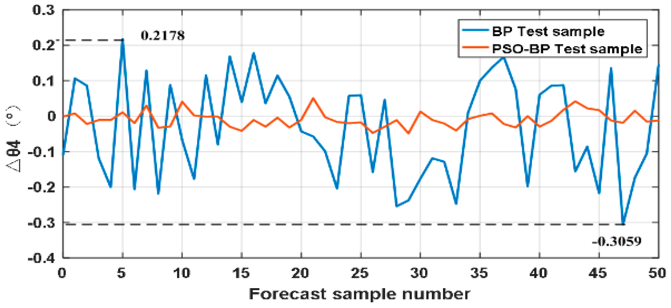
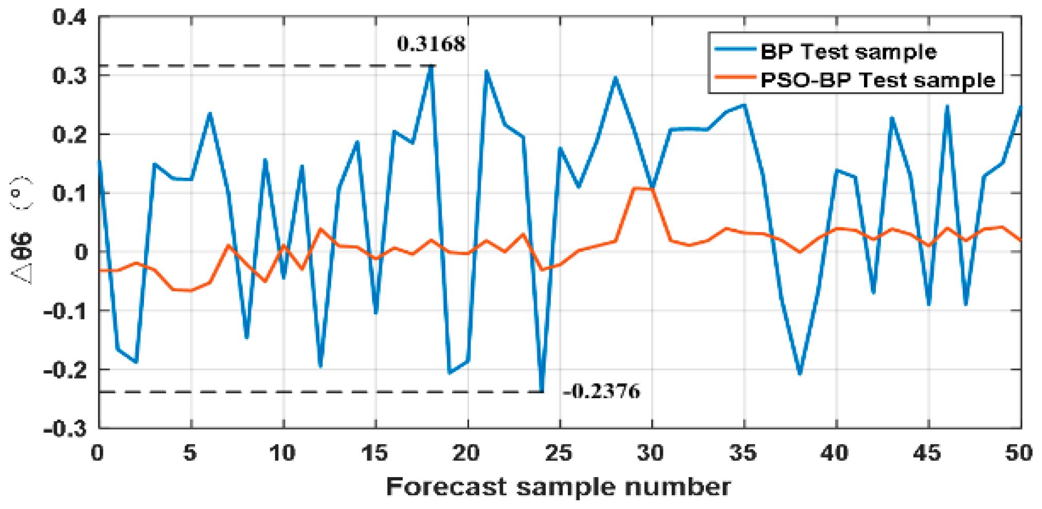
For the network after training, we get the error range of the test set and the range of the mean square error (MSE) which is shown in Table 2. The error range of 50 sets of joint angles, the error range of the joint angle by the BP neural network was calculated as [–0.3059, 0.4130], and the mean square error (MSE) was in the range of [6.72 × 10⁻³, 8.12 × 10⁻²]; the error range of the joint angles by the BP neural network-optimized PSO was calculated as [–0.1859, 0.1079], the mean square error (MSE) was in the range of [2.39 × 10⁻⁴, 6.42 × 10⁻³]. Figure 7, Figure 8, Figure 9, Figure 10, Figure 11 and Figure 12 show the contrast of the BP neural network, and the PSO-BP neural network for the output robot joint angle error △θ. Figure 13 is the comparison of the mean square error (MSE) of the two algorithms.
The experimental results show that, after the machine arm BP optimization PSO neural network obtained by the inverse kinematics of the robot is compared with the BP neural network joint angle error to a high level, the value of the mean square error (MSE) is also enhanced by an order of magnitude. The BP neural network based on PSO optimization is used to solve the inverse kinematics of the manipulator and to verify its effectiveness.
4. Application of the Puncture Robot
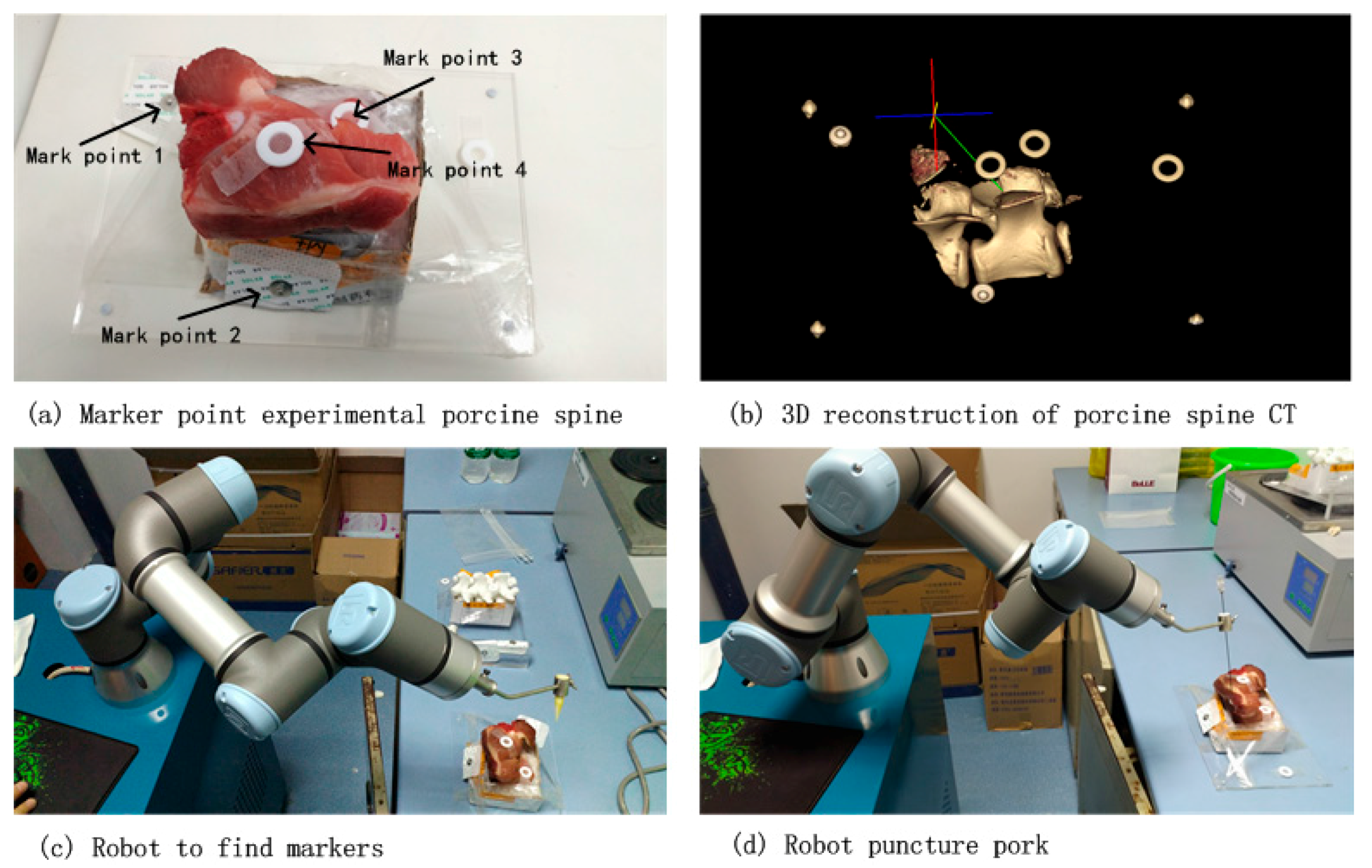
The technology of the puncture robot is new in many research fields, such as medicine, mechanics, imaging, robotics, and so on. This part is based on CT image processing and three-dimensional reconstruction for the guidance and the six degrees of freedom for robot precision positioning technology research; the final step towards completion of medical minimally-invasive surgery with precise positioning control (the principle is shown in Figure 1). The brief process of the experiment is as follows:
- (1)
- Firstly, a piece of porcine spine meat is affixed to some fixed marked points (Figure 14a), and then the DICOM (Digital Imaging and Communications in Medicine)image is obtained by CT scanning.
- (2)
- The CT image is copied to the image processing computer, and the 3D reconstruction is performed on the computer (Figure 14b). Then the coordinates of the marked points in the 3D model are selected.
- (3)
- We can then use, as a coordinate measuring arm, the mechanical measurement of spinal meat marked points on the robot with six degrees of freedom, combined with the coordinates of the marked points in the CT 3D model. Through the space registration conversion, we can obtain the position relationship between the spine meat in the CT 3D model coordinate system, and the robot coordinate system.
- (4)
- The coordinates of the target points and the coordinates of the needle insertion points are selected in the CT 3D model, which determines the route of the needle insertion. The position and rotation in the robot coordinate system are obtained according to the needle insertion route, such as the green line in Figure 14b.
- (5)
- Through the POS-BP neural network algorithm to train the data, we obtain the corresponding joint angles of the robot’s end puncture needle guide pipe when required to reach the specified position and rotation. After the command is sent, the robot moves to the position and ensures its rotation (Figure 14c).
- (6)
- The doctor confirms the positioning of the robot and inserts the needle into the porcine spine (Figure 14d). Once again, through the CT scan of the porcine spine meat, and the reconstruction of the three-dimensional image, a comparison of the needle in the three-dimensional model and the surgical planning of the needle route is conducted, so as to determine the success of the puncture operation.
In this part, we researched the puncture surgery experiment built on porcine spine meat, and verified the PSO-optimized BP neural network algorithm for a robot based on the inverse kinematics problem. The experiment has achieved good results, the accurate positioning of the UR3 robot was ensured within 0.1 mm, and the precision of the robot joint angle was ensured at 0.01 degrees. The results fully met the requirements of the puncture positioning accuracy requirements within 1 mm.
5. Conclusions
In this paper, a hybrid approach has been presented which combines the particle swarm optimization algorithm and BP neural network algorithms to solve the inverse kinematics problem for a six degree manipulator based on end-effector error minimization. The proposed approach combines the characteristics of particle swarm optimization to overcome some inherent defects of BP neural network, and improve the convergence precision of the BP neural network, the convergence speed, and generalization ability. It is difficult to obtain high-precision inverse kinematics solutions because the six DOF robot arm is complex, and there are many problems such as large computational complexity, no guarantee of accuracy, long computation time and so on. In this case, the proposed method will be particularly useful to improve the precision of the result obtained from the PSO-optimized BP neural network algorithm. The joint error and mean square error performance of the PSO-optimized BP neural network are improved by an order of magnitude over the pure BP neural network.
The innovative application of this technology is used in the precise positioning technology of medical puncture surgery; to perform the traditional puncture operation in low precision; to solve poor reliability; to reduce the pain of the patient; to tackle the large labor intensity of the doctor; to eliminate over reliance on the experience of doctors and to address other issues. After obtaining a large number of experimental data, the accuracy can meet the requirements of precise positioning in medical needle surgery, and it has important theoretical and practical value in the research of the key technologies of precise puncturing robots.
Acknowledgments
The authors would like to thank all the reviews for their constructive comments. This work was supported by University of Science and Technology of China, Southwest University of Science and Technology, Key Laboratory of special robot technology of Jiangsu Province for Hohai University, the Institute of Intelligent Manufacturing Technology for Jiangsu Industrial Technology Research Institute.
Author Contributions
Guanwu Jiang and Minzhou Luo conceived and designed the experiments; Keqiang Bai performed the experments; Guanwu Jiang and Saixuan Chen analyzed the data. Guanwu Jiang wrote the paper.
Conflicts of Interest
The authors declare no conflicts of interest.
References
- Yang, G.L.; Kurbanhusen, S.; Yeo, S.H.; Lin, W.; Bin, W. Kinematic design of an anthropomimetic 7-DOF cable-driven robotic arm. Front. Mech. Eng. 2011, 6, 45–60. [Google Scholar] [CrossRef]
- Köker, R. A genetic algorithm approach to a neural-network-based inverse kinematics solution of robotic manipulators based on error minimization. Inf. Sci. 2013, 222, 528–543. [Google Scholar] [CrossRef]
- Bingul, Z.; Ertunc, H.M.; Oysu, C. Applying Neural Network to Inverse Kinematics Problem for 6R Robot Manipulator with Offset Wrist. Coimbra, Portugal, 2005; Springer: Vienna, Austria, 2005; pp. 112–115. [Google Scholar]
- Tabandeh, S.; Clark, C.; Melek, W. A genetic algorithm approach to solve for multiple solutions of inverse kinematics using adaptive niching and clustering. Comput. Sci. Softw. Eng. 2006, 63, 1815–1822. [Google Scholar]
- Hasan, A.T.; Ismail, N.; Hamouda, A.M.S.; Aris, I.; Marhaban, M.H.; Al-Assadi, H.M.A.A. Artificial neural network-based kinematics Jacobian solution for serial manipulator passing through singular configurations. Adv. Eng. Softw. 2010, 41, 359–367. [Google Scholar] [CrossRef]
- Boudjelaba, K.; Ros, F.; Chikouche, D. Potential of Particle Swarm Optimization and Genetic Algorithms for FIR Filter Design. Circuits Syst. Signal Process. 2014, 33, 3195–3222. [Google Scholar] [CrossRef]
- Kalra, P.; Mahapatra, P.B.; Aggarwal, D.K. An evolutionary approach for solving the multimodal inverse kinematics problem of industrial robots. Mech. Mach. Theory 2006, 41, 1213–1229. [Google Scholar] [CrossRef]
- Ayyıldız, M.; Cetinkaya, K. Comparison of four different heuristic optimization algorithms for the inverse kinematics solution of a real 4-DOF serial robot manipulator. Neural Comput. Appl. 2016, 27, 825–836. [Google Scholar] [CrossRef]
- Bernard, C.; Kang, H.; Singh, S.K.; Wen, J.T. Robotic system for collaborative control in minimally invasive surgery. Ind. Robot 1999, 26, 476–484. [Google Scholar] [CrossRef]
- Kebria, P.M.; Al-wais, S.; Abdi, H.; Nahavandi, S. Kinematic and Dynamic Modelling of UR5 Manipulator. In Proceedings of the 2016 IEEE International Conference on Systems, Man, and Cybernetics, Budapest, Hungary, 9–12 October 2016; IEEE: Washington, DC, USA, 2017; pp. 4229–4234. [Google Scholar]
- Hasan, A.T.; Hamouda, A.M.S.; Ismail, N.; Al-Assadi, H.M.A.A. An adaptive-learning algorithm to solve the inverse kinematics problem of a 6 DOF serial robot manipulator. Adv. Eng. Softw. 2006, 37, 432–438. [Google Scholar] [CrossRef]
- Rubio, J.J.; Aquino, V.; Figueroa, M. Inverse kinematics of a mobile robot. Neural Comput. Appl. 2013, 23, 187–194. [Google Scholar] [CrossRef]
- Duguleana, M.; Barbuceanu, F.G.; Teirelbar, A.; Mogan, G. Obstacle avoidance of redundant manipulators using neural networks based reinforcement learning. Robot. Comput. Intergr. Manuf. 2012, 28, 132–146. [Google Scholar] [CrossRef]
- Liu, Y.; Wang, D.Q.; Sun, J.; Chang, L.; Ma, C.X.; Ge, Y.J.; Gao, L.F. Geometric Approach for Inverse Kinematics Analysis of 6-Dof Serial Robot. In Proceedings of the 2015 IEEE International Conference on Information and Automation, Lijiang, China, 8–10 August 2015; IEEE: Washington, DC, USA, 2015; pp. 852–855. [Google Scholar]
- Ma, C.; Zhang, Y.; Cheng, J.; Wang, B.; Zhao, Q.J. Inverse Kinematics Solution for 6R Serial Manipulator Based on RBF Neural Network. In Proceedings of the 2016 International Conference on Advanced Mechatronic Systems, Melbourne, VIC, Australia, 30 November–3 December 2016; IEEE: Washington, DC, USA, 2016; pp. 350–355. [Google Scholar]
- Mayorga, R.V.; Sanongboon, P. Inverse kinematics and geometrically bounded singularities prevention of redundant manipulators An Artificial Neural Network approach. Robot. Auton. Syst. 2005, 53, 164–176. [Google Scholar] [CrossRef]
- Kennedy, J.; Eberhart, R. Particle Swarm Optimization. In Proceedings of the IEEE International Conference on Neural Networks IV, Perth, Australia, 27 November–1 December; IEEE: Piscataway, NJ, USA, 1995; pp. 1942–1948. [Google Scholar]
- Chen, C.C.; Li, J.S.; Luo, J.; Xie, S.R.; Li, H.Y. Seeker optimization algorithm for optimal control of manipulator. Ind. Robot 2016, 43, 677–686. [Google Scholar] [CrossRef]
- Si, L.; Wang, Z.W.; Liu, Z.; Liu, X.H.; Tan, C.; Xu, R.X. Health Condition Evaluation for a Shearer through the Integration of a Fuzzy Neural Network and Improved Particle Swarm Optimization Algorithm. Appl. Sci.-Basel 2016, 6, 171. [Google Scholar] [CrossRef]
- Falconi, R.; Grandi, R.; Melchiorri, C. Inverse Kinematics of Serial Manipulators in Cluttered Environments using a new Paradigm of Particle Swarm Optimization. IFAC Proc. Vol. 2014, 47, 8475–8480. [Google Scholar] [CrossRef]
- Kuo, P.H.; Liu, G.H.; Ho, Y.F.; Li, T.H.S. PSO and Neural Network based Intelligent Posture Calibration Method for Robot Arm. In Proceedings of the 2016 IEEE International Conference Systems, Man, and Cybernetics (SMC), Budapest, Hungary, 9–12 October 2016; IEEE: Washington, DC, USA, 2016; pp. 003095–003100. [Google Scholar]
Figure 1.
Position principle of the puncturing robot.

Figure 2.
The real UR3 manipulator.

Figure 3.
Schematic and frame assignment of UR3 (θi = 0 for 1 ≤ i ≤ 6).
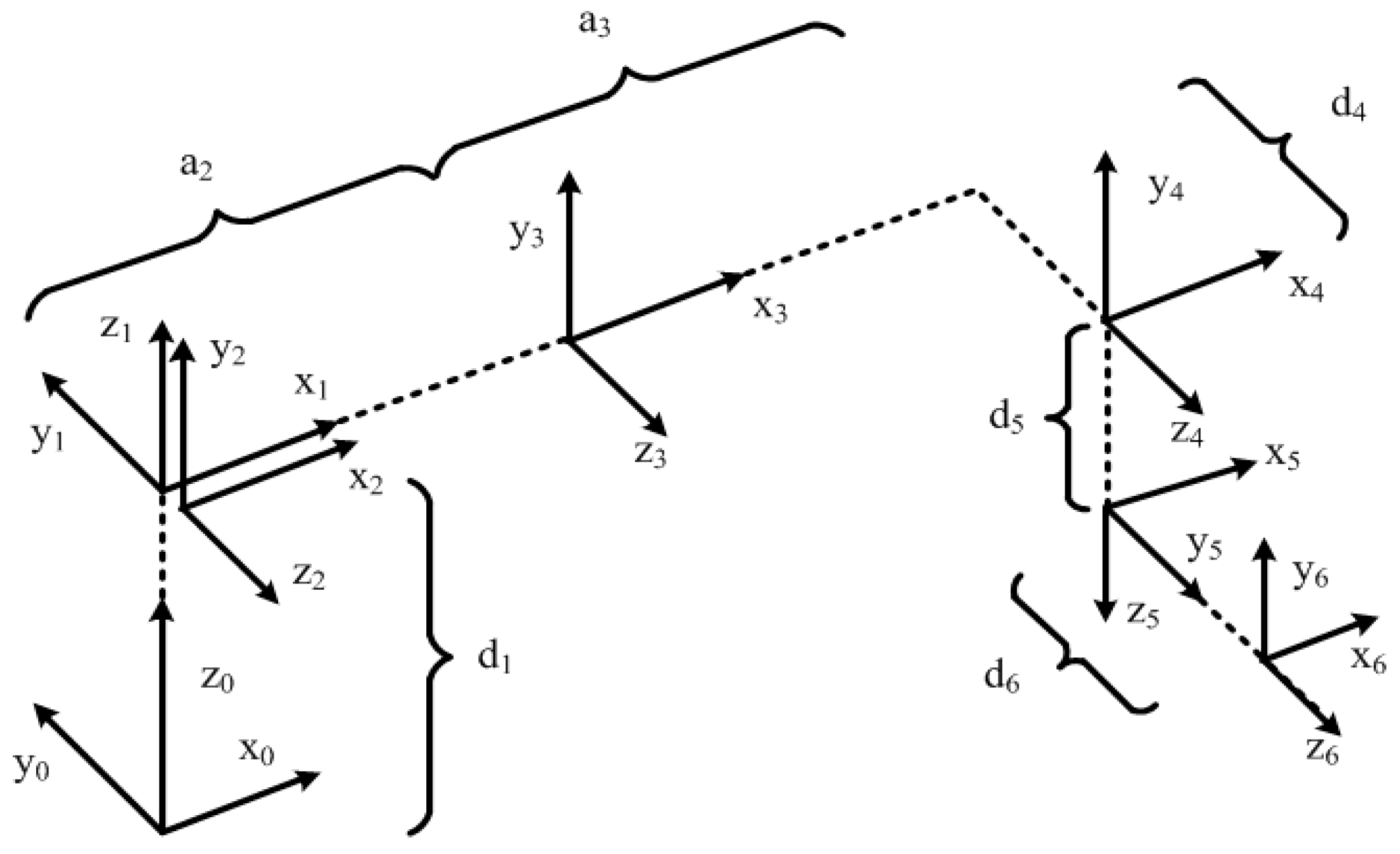
Figure 4.
Model of an artificial neuron.
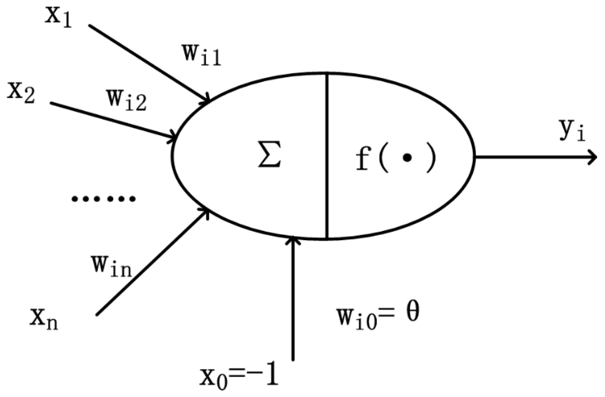
Figure 5.
BP (back propagation) neural network topology structure.
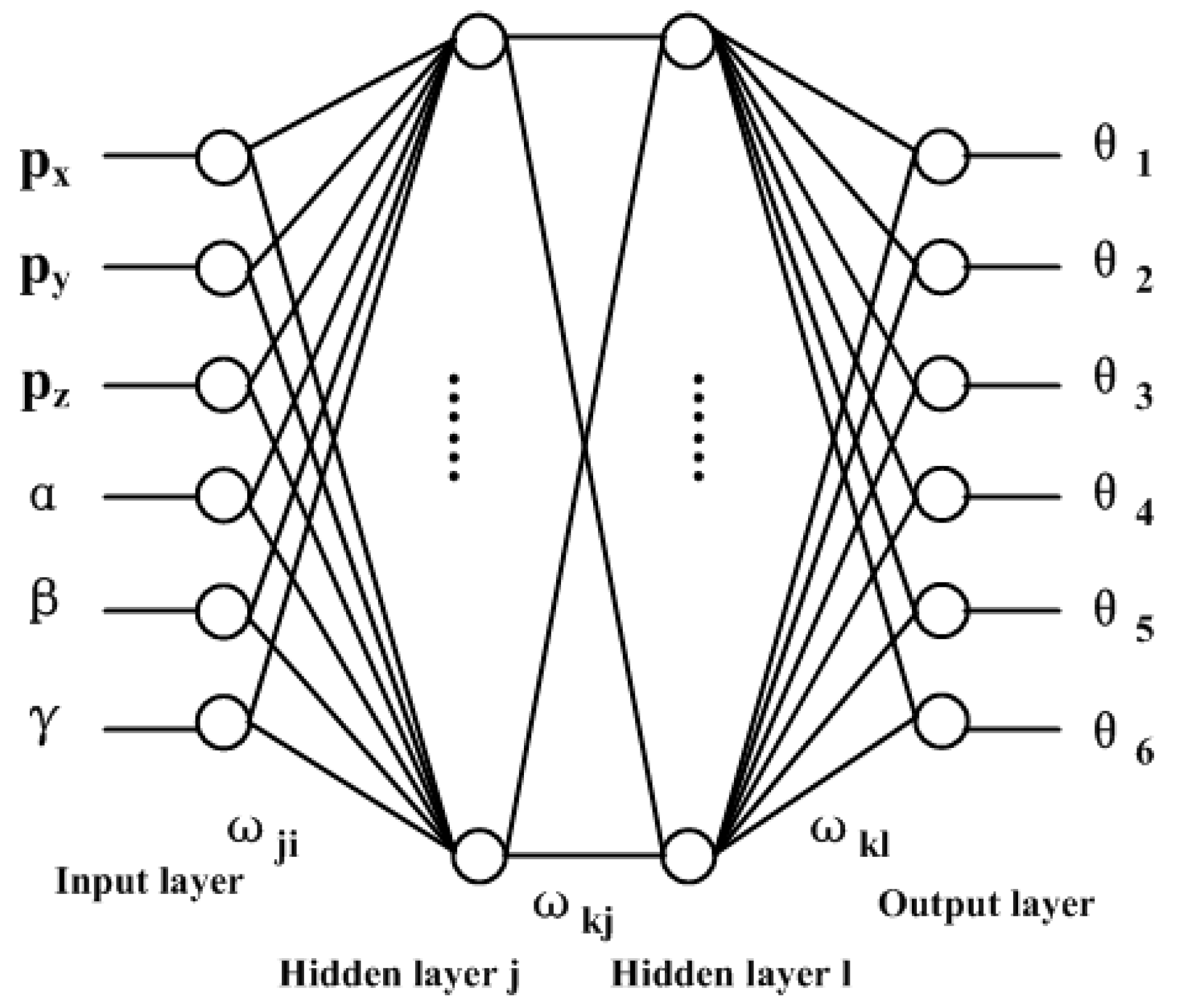
Figure 6.
PSO (particle swarm optimization) optimization and BP neural network flowchart.
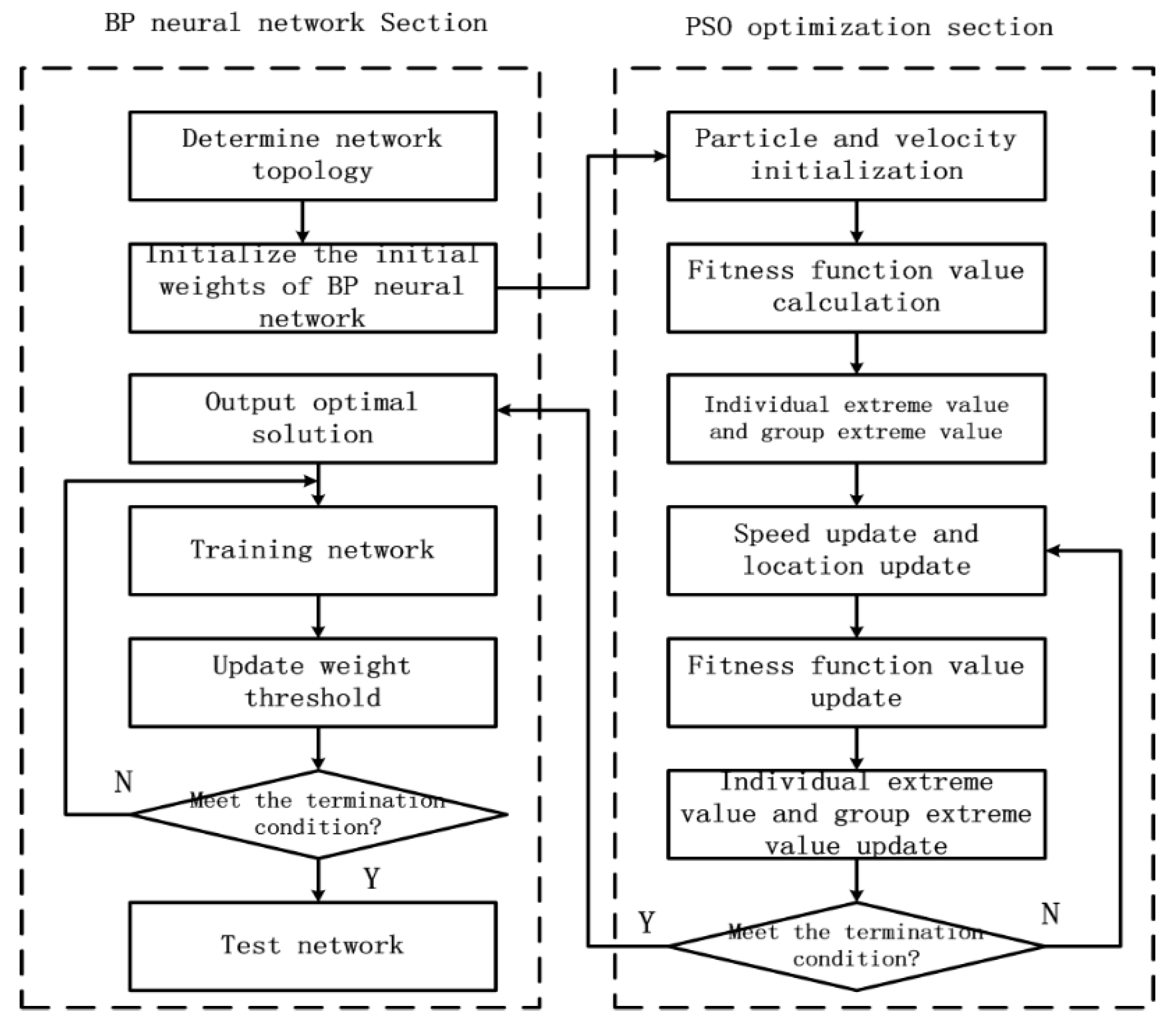
Figure 7.
Error contrast of test set’s θ1.

Figure 8.
Error contrast of test set’s θ2.
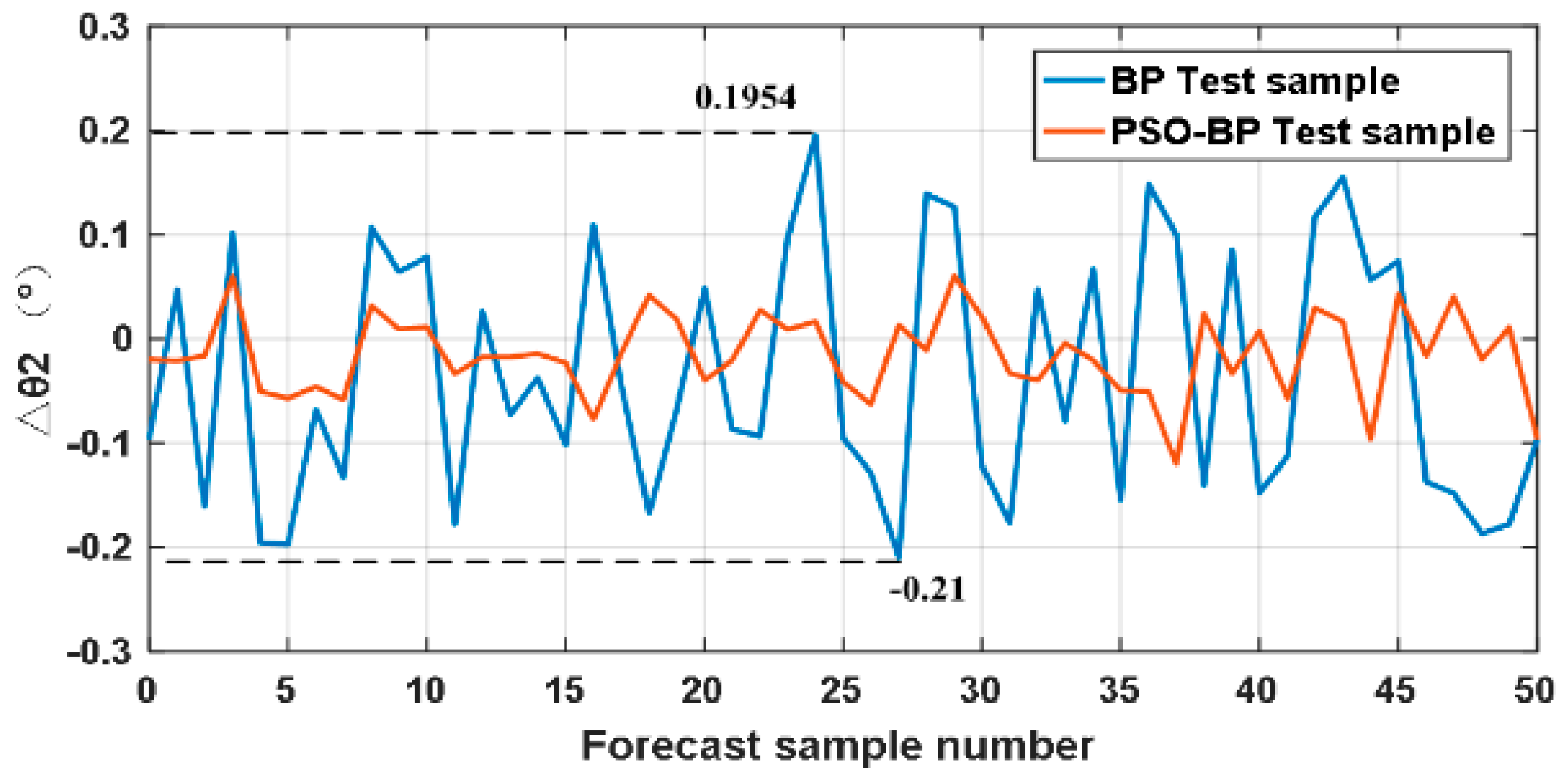
Figure 9.
Error contrast of test set’s θ3.
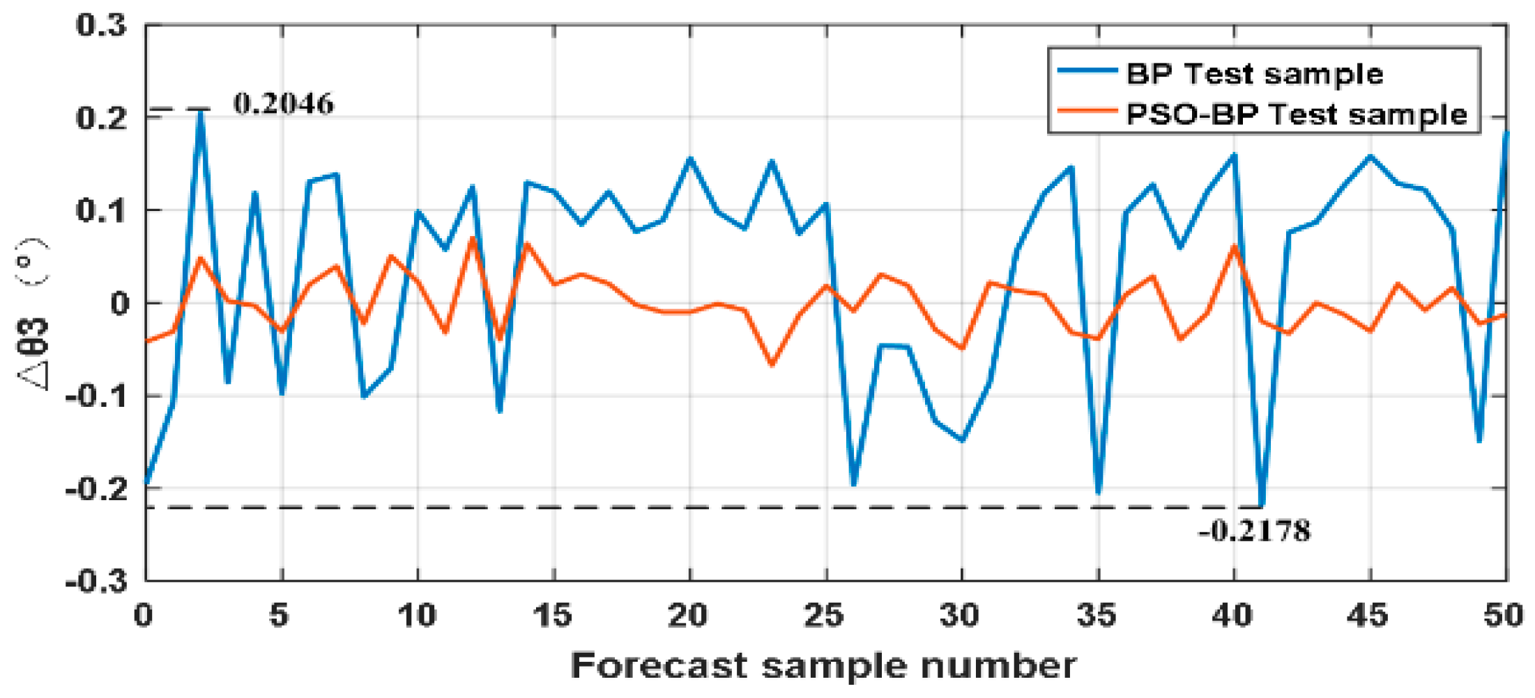
Figure 10.
Error contrast of test set’s θ4.

Figure 11.
Error contrast of test set’s θ5.
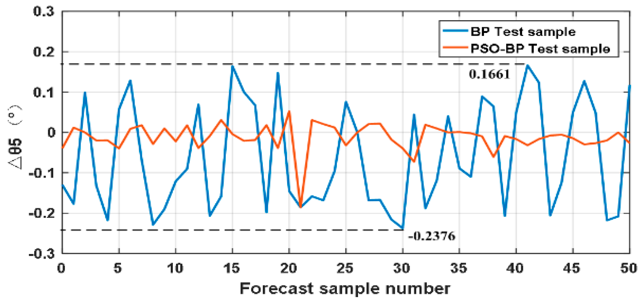
Figure 12.
Error contrast of test set’s θ6.

Figure 13.
Mean square error (MSE) contrast of test set’s θ.
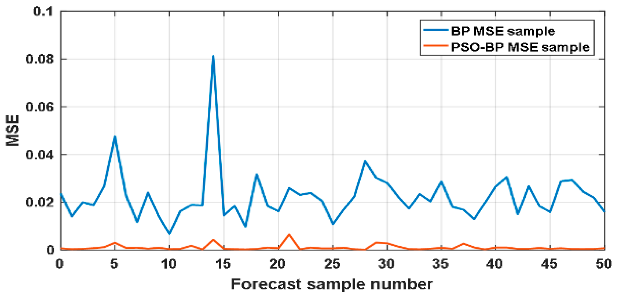
Figure 14.
UR3 robot puncture process chart.

Table 1.
Denavit-Hartenberg (D-H) parameters for the UR3 robot.
| Link | θ (rad) | a (mm) | d (mm) | α (rad) |
|---|---|---|---|---|
| Joint 1 | 0 | 151.9 | π/2 | |
| Joint 2 | –243.65 | 0 | 0 | |
| Joint 3 | –213.25 | 0 | 0 | |
| Joint 4 | 0 | 112.35 | π/2 | |
| Joint 5 | 0 | 85.35 | –π/2 | |
| Joint 6 | 0 | 81.9 | 0 |
Table 2.
Error range test set and mean square error.
| Joint Angles and MSE (Mean Square Error) | BP (Back Propagation) Neural Network | PSO (Particle Swarm Optimization)-BP Neural Network |
|---|---|---|
| Δθ1 | −0.2005–0.4130 | −0.0534–0.065 |
| Δθ2 | −0.2100–0.1954 | −0.1199–0.0605 |
| Δθ3 | −0.2178–0.2046 | −0.0672–0.0704 |
| Δθ4 | −0.3059–0.2178 | −0.0486–0.0508 |
| Δθ5 | −0.2376–0.1661 | −0.1859–0.0526 |
| Δθ6 | −0.2376–0.3168 | −0.0658–0.1079 |
| MSE | 6.72 × 10⁻³–8.12 × 10⁻² | 2.39 × 10⁻⁴–6.42 × 10⁻³ |
© 2017 by the authors. Licensee MDPI, Basel, Switzerland. This article is an open access article distributed under the terms and conditions of the Creative Commons Attribution (CC BY) license (http://creativecommons.org/licenses/by/4.0/).
Share and Cite
MDPI and ACS Style
Jiang, G.; Luo, M.; Bai, K.; Chen, S. A Precise Positioning Method for a Puncture Robot Based on a PSO-Optimized BP Neural Network Algorithm. Appl. Sci. 2017, 7, 969. https://doi.org/10.3390/app7100969
AMA Style
Jiang G, Luo M, Bai K, Chen S. A Precise Positioning Method for a Puncture Robot Based on a PSO-Optimized BP Neural Network Algorithm. Applied Sciences. 2017; 7(10):969. https://doi.org/10.3390/app7100969
Chicago/Turabian StyleJiang, Guanwu, Minzhou Luo, Keqiang Bai, and Saixuan Chen. 2017. "A Precise Positioning Method for a Puncture Robot Based on a PSO-Optimized BP Neural Network Algorithm" Applied Sciences 7, no. 10: 969. https://doi.org/10.3390/app7100969
Note that from the first issue of 2016, this journal uses article numbers instead of page numbers. See further details here.