Low Reynolds Number Flow Around Tori of Different Slenderness Γ
by
 and
and
Werner M. J. Lazeroms
1, 
Marco D. De Tullio
2,
Nicola De Santis
2,
Roberto Pizzoferrato
3,* and
Roberto Verzicco
3 1
Institute for Marine and Atmospheric Research Utrecht, Utrecht University, PO Box 80.005, 3508 TA Utrecht, The Netherlands
2
Dipartimento di Meccanica, Matematica e Management, Politecnico di Bari, Via Re David 200, 70125 Bari, Italy
3
Dipartimento di Ingegneria Industriale, Università di Roma ‘Tor Vergata’, Via del Politecnico 1, 00133 Roma, Italy
*
Author to whom correspondence should be addressed.
Appl. Sci. 2017, 7(11), 1108; https://doi.org/10.3390/app7111108
Submission received: 25 September 2017
/
Accepted: 20 October 2017
/
Published: 26 October 2017
(This article belongs to the Section Mechanical Engineering)
Abstract
:We present the results of axisymmetric and three-dimensional numerical simulations of the flow around a torus in the low Reynolds number regime ; and aspect-ratio (core diameter over toroidal radius). It is shown that as , consistent with intuition and the results from the literature, the flow tends to that of a two-dimensional circular cylinder while for the flow is that around a bluff obstacle. It has been observed that in a small region of the – phase space, the flow develops an axisymmetric recirculation detached from the torus and with a vorticity distribution that resembles the Hill vortex. In the range , several different regimes have been observed; the peculiarities of each regime are analyzed and, whenever possible, similarities and differences with other classical flows are discussed.
1. Introduction
Flows around circular cylinders and spheres have been attracting the interest of researchers for more than a century owing to their relatively easy and controllable conditions, as well as the interesting flow physics [1,2]. These problems have often been considered as prototypes of flows around bluff bodies which are relevant to engineering and practical applications. In these cases, the body geometry is described by a single parameter (the diameter d of the cylinder or of the sphere) and the flow is characterized only by the Reynolds number , with U the free stream velocity and the kinematic viscosity of the fluid.
A possible extension of the above flow paradigms consists of considering a geometry that is described by two curvature parameters instead of one. We believe that in this way it is possible to establish the standard for a new benchmark that, even if yet to be well defined and sufficiently simple, shows a richer and more complex flow physics with respect to circular cylinders and spheres.
In the present paper we have considered the flow around a toroidal ring with radius R and core diameter in an attempt to increase the complexity of the problem. In fact, it is possible to change, in addition to the Reynolds number , also the slenderness parameter . Apart from the paper by [3] that used a rarefied hypersonic flow, this problem has been considered for an incompressible flow by several studies in the past. Reference [4] considered “fat” tori () in the Stokes regime, while [5] investigated only slender tori (low ) in the very low Reynolds number range. Reference [6] conducted experiments to measure the drag in axisymmetric conditions, and [7,8,9] performed accurate and extensive numerical simulations and stability analyses showing that all the dynamics from the flow around a sphere () to that around a circular cylinder () can be obtained by varying the cylinder slenderness.
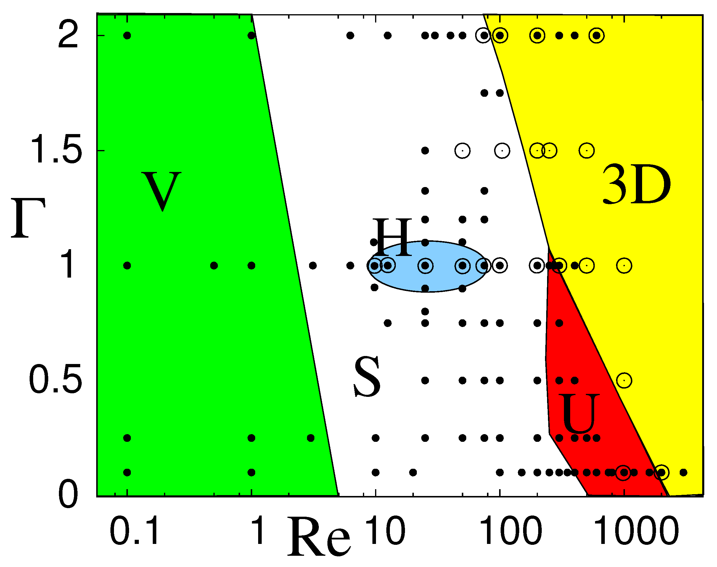
In this study we have analyzed the low Reynolds number range ; , and the aspect ratio has been spanned from up to the limit ; the results are summarized in the phase diagram of Figure 1, confirming that indeed the aspect ratio plays a fundamental role in the determination of the flow features. The novel finding of this study is the existence of a new regime in the – phase space, indicated by H in Figure 1. In this region the flow develops a spherical vortex in the wake detached from the surface of the torus, whose vorticity is distributed as in the Hill spherical vortex [10].
It is worth mentioning that the phase diagram of Figure 1 has been obtained from the results of about 100 numerical simulations, more than 20 of which are fully three-dimensional. The boundaries between the regions have been somehow arbitrarily set by observing the flow behaviour and gathering the simulations into homogeneous categories. Therefore, the lines dividing the different regions should not be interpreted as sharp fronts, but rather as regions where the transition occurs.
2. Problem and Numerical Setup
In this paper, the Navier–Stokes equations for an incompressible viscous flow are numerically integrated; their nondimensional forms read:
with the velocity, p the pressure, the material derivative, and a forcing for the immersed boundary method (specified later). Equation (1) have been spatially discretized in a cylindrical coordinate system using staggered central second-order accurate finite-difference approximations. Details of the numerical method are given in [11], and only the main features are summarized here. The discretized system is integrated using a fractional-step method where the viscous terms are computed implicitly and the convective terms explicitly. At each time step, the momentum equations are provisionally advanced in time using the pressure at the previous time step, giving an intermediate non-solenoidal velocity field. A scalar quantity is then introduced to project the non-solenoidal field onto a solenoidal one. A hybrid low-storage third-order Runge–Kutta scheme is used to advance the equations in time.
The forcing of Equation (1) is introduced to handle complex geometric configurations without a body conformal mesh; this is the immersed boundary method whose details can be found in [12]. In a few words, if Equation (1) is rewritten as , with containing the advective, pressure, and viscous terms, its time discrete version reads:
Here the superscripts indicate the discrete time levels and indicates the midpoint between times and . If at the immersed boundary the fluid velocity is imposed as , Equation (2) can be explicitly solved for , yielding
which is imposed at all immersed interface nodes while it results everywhere else. This procedure allows the imposition of a velocity boundary condition on an arbitrary surface, and is consistent with the centered second-order finite-difference approximation; therefore, the overall accuracy of the scheme remains second-order [12].
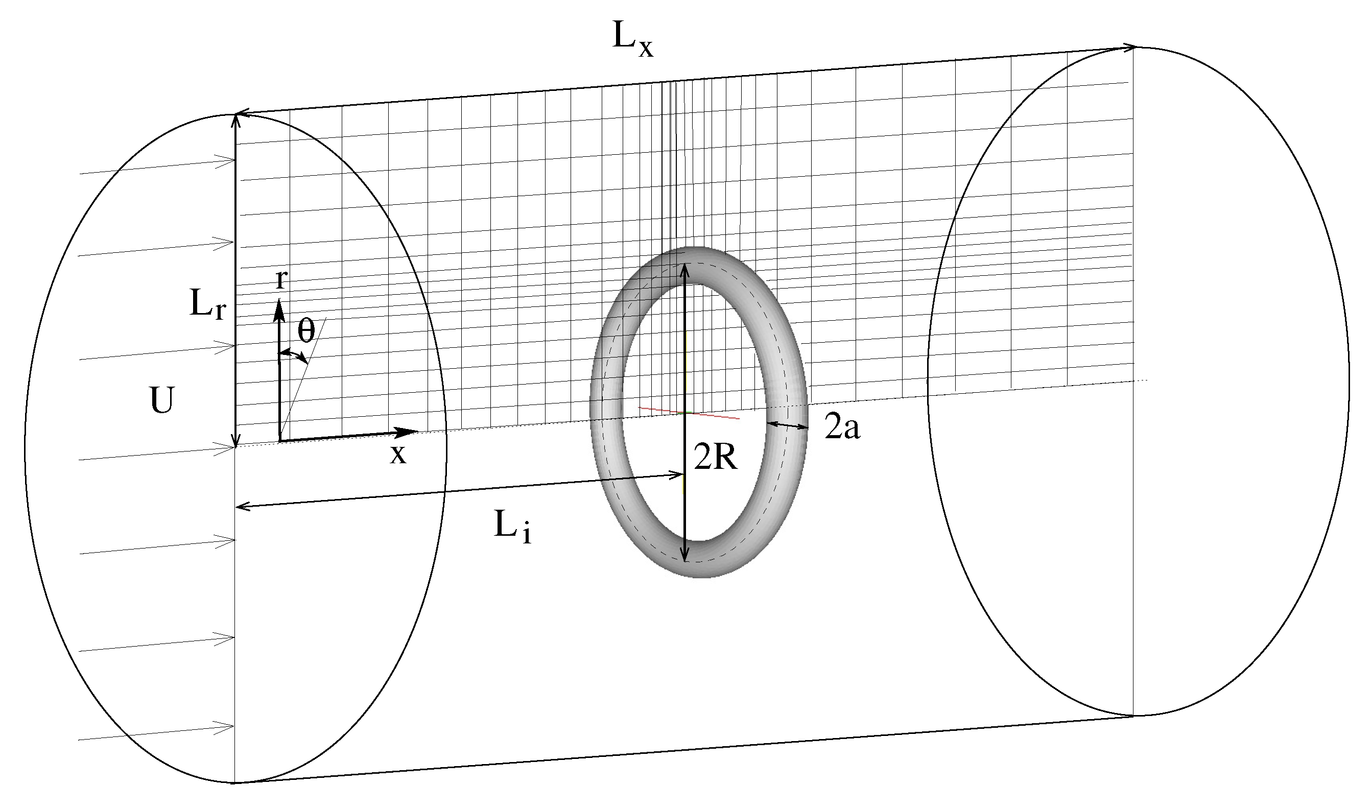
The problem is sketched in Figure 2, and is summarized as follows: a torus of radius R and core radius a is normally placed along the axis of a cylindrical domain of radius and length , respectively, in the radial r and axial x directions. The torus is at a distance from the inflow (). The flow boundary conditions are:
In the boundary conditions at (), all the velocity components are advected outside the domain with a velocity c which is dynamically determined so as to assure the free-divergence of the velocity field at every time step.
The computational domain is discretized by a mesh which is non-uniform in the radial and axial directions to cluster the gridpoints in the torus region and in the wake (see the example in the sketch of Figure 2); for the three-dimensional cases, the mesh is uniform in the azimuthal direction. The axisymmetric cases have been mainly run on two different grids and in the radial and axial directions, respectively, obtaining a drag coefficient (computed by integrating viscous stresses and pressure over the torus surface and projecting the normalized force in the streamwise direction) that typically showed a difference below . In many cases—especially those with low and high —a third grid of nodes has been used to further assess the grid independence of the results again with differences below , which is within the statistical uncertainty of the data.
The standard domain dimensions are and , with the inflow distance ; however, since the ideal flow consists of an isolated torus, we have verified that the domain finiteness did not significantly affect the results through the blockage effect. In more detail, the cases at for and have also been run using a second domain of dimensions and , and the number of nodes augmented accordingly: the differences in the drag coefficient now below . In a second test it has been verified that the torus was placed far enough from the inflow to have results independent of : this was checked by repeating the runs at and and with and on a grid extended ahead of the torus; in this case, the maximum difference of the drag coefficient was below , which is acceptable for our purposes.
Owing to the large CPU requirements, only a few three-dimensional cases were run, and all of them on the standard domain with a grid in the radial, axial, and azimuthal directions. These last runs were mainly aimed at showing the onset of three-dimensional instabilities rather than analyzing the flow details.
A first validation of the results is given by the analytical study of [4], who computed the Stokes flow around a “closed” torus () for which they found a drag coefficient ; the present numerical results yield at and at , which are in very good agreement with the prediction.
A further validation is provided in Figure 3 showing the drag coefficient (i.e., the force in the opposite direction with respect to the mean flow normalized by the factor , with S the blockage area) as function of the Reynolds number. The results are compared with the classical paper by [13], and the deviations range from a minimum of at up to a maximum of at . It is worth mentioning that the validation in the range is much more challenging than that at low Reynolds, owing to the steeper velocity gradients in the flow and the thinner boundary layers at the sphere surface. Further validation is shown in the next section for different aspect-ratios and Reynolds number ranges. Here it suffices to mention that the results of Figure 3 confirm that the numerical tool is reliable and the criteria for the selection of the run parameters (grid spacing and time step) are adequate.
3. Results
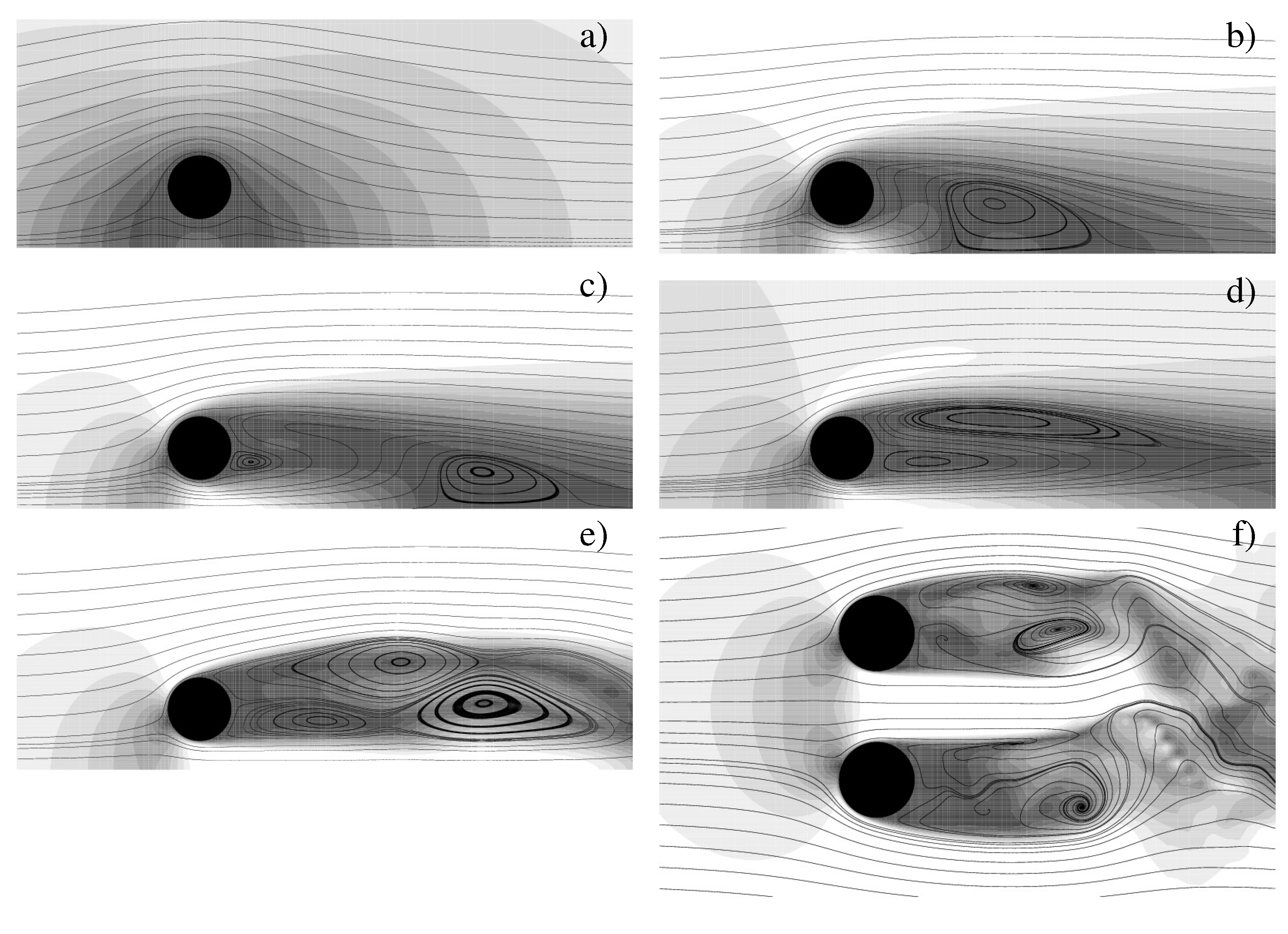
In order to make the discussion easier, we will briefly illustrate first the flow evolution for a fixed aspect ratio () as a function of the Reynolds number. For , the dynamics is dominated by viscosity with the flow smooth and steady, without separations; this is the Stokes regime (Figure 4a), where between the upstream and downstream flows there is an approximate symmetry that becomes more exact the more . As Re is increased, the flow remains steady and a first recirculation can appear: however, this recirculation is not attached to the torus, but located downstream in the wake. This regime is generated by the competing effects of blockage of the torus and downstream convection of the mean flow. Owing to the vorticity distribution within the bubble, it will be referred to as Hill regime, and it can exist only in a narrow range of aspect ratios (around ) and Reynolds numbers (Figure 4b). A further increase of produces separations attached to the torus that in some cases can coexist with the Hill recirculation (Figure 4c), but eventually only recirculations attached to the torus surface can survive (Figure 4d). When the Reynolds number is still augmented, the flow becomes unsteady (Figure 4e) with a wake that oscillates in time and sheds compact vortices. The last regime is observed for even higher when the flow becomes three-dimensional and also the azimuthal symmetry is lost (Figure 4f).
The above scenario can change considerably depending on the aspect ratio of the torus: in the following sections, we will illustrate the flow dynamics in the various regimes for different values of .
3.1. Stokes Regime
The first regime is that of very low Reynolds numbers characterized by dominating viscous effects that determine the flow. In this context, the governing dynamics is a balance between pressure and viscous forces that is expressed by the Stokes equation ; this does not have inertial terms, and therefore cannot involve the fluid density . On the other hand, the drag force is commonly written as , with S a reference surface that—for this problem—is the blockage area . The only way for to get rid of is that , and this is a common feature of all very low flows. Figure 5 shows that indeed also for the torus the drag coefficient follows this power law; here, in the interest of brevity, we show only the results for and even if the scaling is observed for all values of .
For small aspect ratios , the flow tends to that around a two-dimensional cylinder () and, accordingly, already for the is almost indistinguishable from that for a circular cylinder. It is worth noting that the Reynolds number for the cylinder is defined with the cylinder diameter, while here we use the toroidal radius R; this implies that the two Reynolds numbers are related through , which should be kept in mind when comparing the two flows.
The behaviour is qualitatively similar for the aspect ratio , although the fits have different coefficients than for the two-dimensional cylinder: here we have found in the Stokes regime . We report for comparison the data for the same flow computed in [9], which show a perfect agreement with the present ones.
3.2. Hill Regime
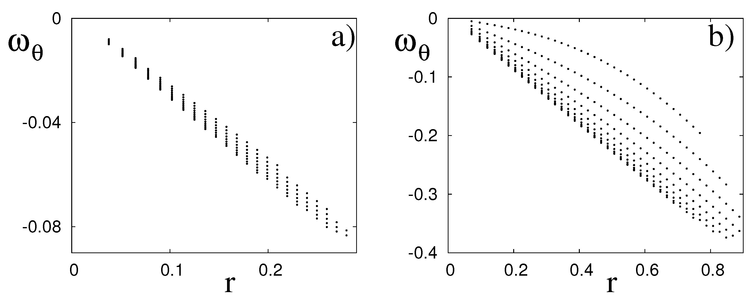
For , some values of the Reynolds number gave rise to a special steady state which, to the knowledge of the authors, has never been reported before. More in detail, at the flow at showed the appearance of a recirculation bubble in the wake of the torus, the bubble consisting of a vortex ring (Figure 6a,b). The shape of this ring is approximately spherical at its onset, but it becomes more elongated in the streamwise direction for increasing owing to its interaction with the strain field produced by the torus. In fact, this recirculation shows strong similarities with the Hill spherical vortex [10] that is characterized by a linear azimuthal vorticity distribution , with r the radial coordinate and A a constant. In view of this similarity, we have verified whether this relation also holds for the recirculation of the torus, and two representative results are shown in Figure 7. It is clear that at , when the vortex is approximately spherical and not strained by the flow, the linear relationship is attained very closely (note that in Figure 7 the axes do not have the same range in both panels). On the other hand, at the bubble is significantly elongated in the streamwise direction (Figure 4c) and partially stripped by the external strain field; accordingly, the relation shows evident deviations from linearity—especially in the upstream part of the vortex that is more subject to the wake of the torus.
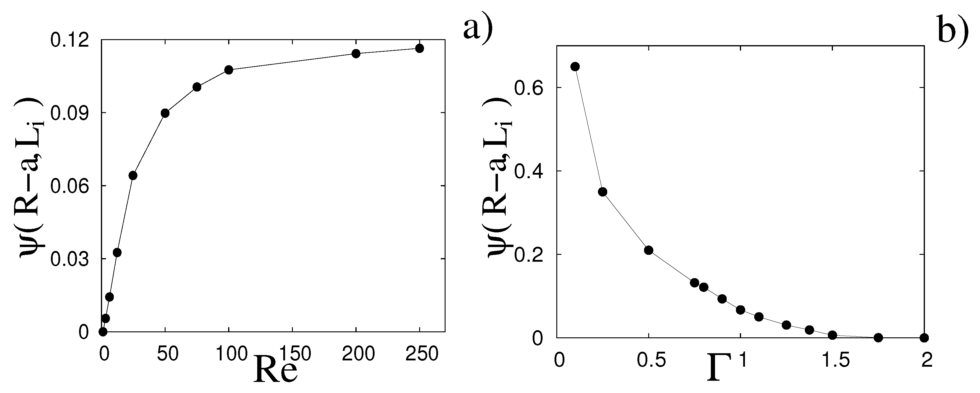
As a successive step, we analyze how the recirculation is generated: it is expected that the appearance and disappearance of the vortex is somehow related to the relative proportions of fluid passing over and through the torus. As measure of the flux, we have computed the Stokes streamfunction that, computed for and , yields the flow passing through the torus (inner flux). Some results are reported in Figure 8, showing an increase of the flux with and a tendency to saturation at “high” Reynolds number. It is also evident that this flux decreases for increasing , since the torus tends to be “fat” and the surface of the central hole diminishes. Figure 6d clearly shows that when this flux is vanishing the bubble attaches to the torus as for the separation behind a bluff body. On the other hand, for low values of , the inner flux is too intense to allow for an axial steady separation. Therefore, it turns out that this regime can only exist for some combinations of and to have an inner flux strong enough to produce a recirculation (through the adverse pressure gradient downstream of the torus) but not too strong to wash it away. The – values for which this special steady state was found are contained within the region H of Figure 1.
3.3. Steady Regime
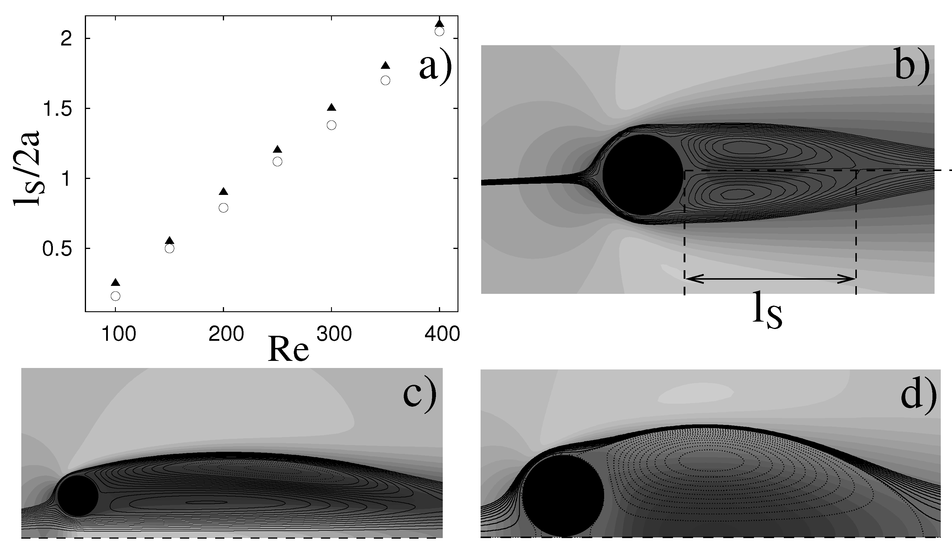
Apart from the limited range of where the Hill regime can exist, after the Stokes region of the – phase space we find a steady regime in which stationary separation bubbles appear downstream attached to the torus. It has been observed that for , already at a small recirculation is present while for only above does a separation appear. In the first case, the flow is characterized by a single bubble that grows for increasing , and it remains steady up to (Figure 9d). As is decreased, two counter-rotating recirculations develop with the inner one (that closer to the axis of symmetry) smaller than the external one (Figure 9c). This difference decreases as is diminished, and for any difference between the bubbles should disappear since the two-dimensional cylinder case is recovered. Our simulations at show that indeed the flow approaches the cylinder limit even if differences are still present. In particular, Figure 9a reports the length of the separation bubble (measured as the distance from the back of the torus where the streamwise velocity reverts its sign as in Figure 9b) as function of compared with the analogous quantity for the plane cylinder. It is observed that the results are very close even if the data for the torus are systematically below those for the cylinder. After having verified that this effect is not related to insufficient numerical resolution or to the finiteness of the computational domain, we have found that this difference is caused by the finite aspect ratio that produces a blockage of the inner flow. In other words, the flow going through the torus is accelerated more than the flow going over, thus pushing the separation towards the rear of the torus surface and consequently decreasing the length of the separation. This argument is in agreement with the recent paper by [14] that computed the flow around a circular cylinder over several domains, and they have observed that indeed the length of the steady separation bubble is reduced for increasing blockage of the flow. These results are qualitatively and quantitatively consistent with those of [7,8,9].
3.4. Unsteady Regime
A further increase of the Reynolds number enhances the inertial effects with respect to the viscous ones, and this induces flow transition from steady to unsteady. The recirculations that in the steady regime were attached to the torus are now alternatively shed in the wake and advected by the main flow. A typical case is shown in Figure 10 for the aspect ratio and , and it is similar to the flow around a circular cylinder.
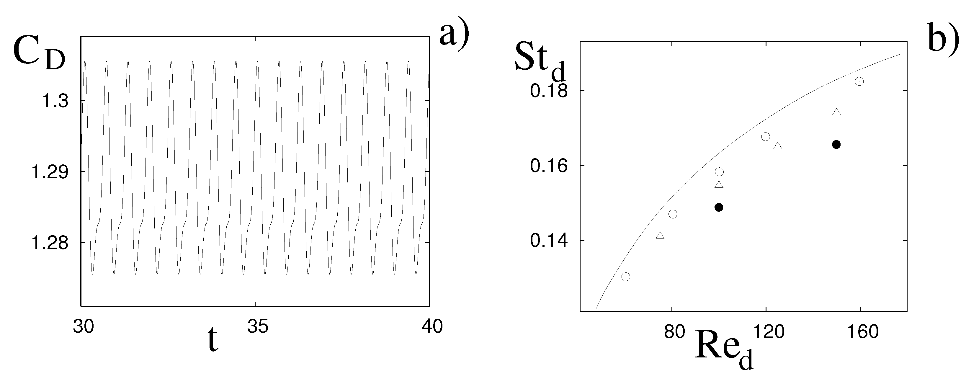
A characteristic quantity of the unsteady vortex street is the Strouhal number , where f is the main frequency of the flow. Here f has been measured from the first peak of the fast Fourier transform of the drag coefficient (Figure 11a), even if any other quantity (for example, velocity or pressure sampled in a point) yielded the same result. Similarly to the Reynolds number, the relation has been used to compare the present results with those of a circular cylinder, since the Strouhal number for a cylinder is computed using the cylinder diameter. Figure 11b shows the normalized oscillation frequencies of the flow as a function of the Reynolds number, and in order to make the comparison easier, all the data are normalized in the same way as for the circular cylinder. For , the Strouhal number for the torus appears to be close to the corresponding value for the cylinder, yet systematically below it. Similarly to the separation length of Figure 9a, also in this case the difference is due to the finiteness of the aspect ratio and this is confirmed by the analogous quantities for and showing larger discrepancies and in the same direction as the case at .
Another fundamental difference between the wake of a cylinder and that of a torus is that the vortices of the latter are in fact vortex rings, and they have a self-induced translation velocity that adds (algebraically) to the convection of the wake. For a vortex ring with thin core and uniform vorticity distribution within the core, the self-induced translation velocity is , where is the core circulation, b the ring radius, and the core radius. Looking at Figure 10, we can see that the vortices shed from the external side rotate clockwise while the others rotate counterclockwise; this implies that the internal vortices must travel downstream faster than the external ones, and accordingly the wake tends to diverge radially as shown by the straight lines connecting the vortex centres. This behaviour is different from that of the cylinder, whose wake spreads symmetrically with respect to the streamwise direction.
In the case at , the internal and external vortices have very similar dimensions, and the measured differences of were below . However, the situation becomes different as increases because the external vortices increase in size at the expense of the inner vortices that eventually disappear. This completely changes the instability mechanisms, and tends to inhibit the flow unsteadiness. Figure 11b shows that indeed for a given the oscillation is slower for increasing , and we have found that for the axisymmetric unsteadiness is suppressed with a direct transition from steady axisymmetric to three-dimensional flows (Figure 1).
3.5. Three-Dimensional Regime
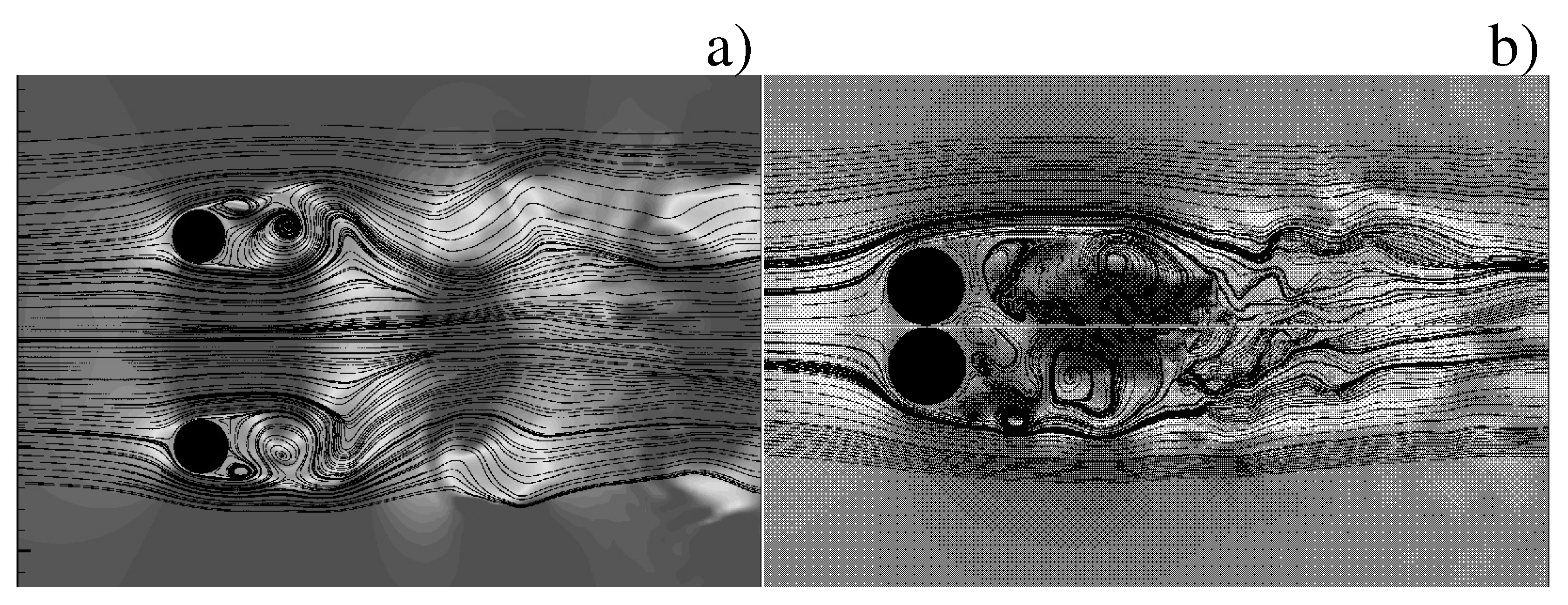
Beyond the unsteady regime the flow loses the axial symmetry and it becomes completely three-dimensional; examples of flow snapshots are given in Figure 4f and Figure 12 for three different aspect ratios. We have seen in the previous section that the flow features are strongly influenced by , and this is also confirmed in the three-dimensional case where the flow instability depends on the topological structure of the separation. In order to clearly distinguish between truly axisymmetric and marginally three-dimensional flows, we have checked all the force and moment components. In the former case, all coefficients except for the drag assumed zero values (the computer round-off error), while for three-dimensional flows—though small and with zero time average—every coefficient was different from zero. Further flow analysis would require the investigation of the azimuthal instabilities of the ring vortices in the wake and their interaction. However, this kind of analysis is quite complex; it would deserve a dedicated study that is beyond the purposes of this paper. Here we only aimed at finding the region of the three-dimensional flow dynamics in the phase diagram of Figure 1.
4. Conclusions
This paper has analyzed the flow around a toroidal ring at low with the aim of proposing a new benchmark that is more complex than the classical circular cylinder and sphere yet sufficiently simple and well-defined to allow a detailed investigation. The – phase diagram reported in Figure 1 shows that several different regimes are possible, and they span from the Stokes dynamics up to the fully three-dimensional flow. For , the flow tends to become that around a circular cylinder, while as the torus aspect ratio increases the differences between internal and external flows become dominant. For , the inner flow is inhibited, only a single separation behind the torus is generated, and the flow resembles that around an obstacle. A particular steady flow referred to as Hill regime has been found for a limited range of and in which a recirculation downstream in the wake (but not attached to the torus) is present.
Before concluding this paper we wish to point out that the boundaries of the phase diagram of Figure 1 must be intended only as indicative transitional zones rather than sharp limits. For example, looking at Figure 6a,b it appears that increasing has the effect of moving the recirculation upstream towards the torus until it attaches to its surface; for intermediate , the distinction between a simple massive steady separation from a highly strained Hill vortex is certainly questionable. In addition, the cases delimiting the unsteady regions are considerably more computationally expensive than others, since distinguishing between very slowly decaying disturbances from a marginally sustained perturbation requires an integration over several viscous time scales that—especially for high- flows computed on fine grids—becomes infeasible. For example, a typical simulation in the Stokes or steady viscous regime can be run on a single processor desktop computer within 2–4 CPU h, while in the unsteady regime, in order to collect enough statistics, the CPU time increases up to 20–30 h. If a full three-dimensional unsteady case is considered, the CPU time ramps up to 300–500 h and parallel computing is needed.
Acknowledgments
The paper was prepared with the financial support of CEMeC of Politecnico di Bari.
Author Contributions
All the authors have equally contributed to the development of the numerical code, the simulations and the analysis of the data.
Conflicts of Interest
The authors declare no conflict of interest.
References
- Johnson, T.A.; Patel, V.C. Flow past a sphere up to a Reynolds number of 300. J. Fluid Mech. 1999, 378, 19–70. [Google Scholar] [CrossRef]
- Williamson, C.H.R. Vortex dynamics in the cylinder wake. Annu. Rev. Fluid Mech. 1996, 28, 477–539. [Google Scholar] [CrossRef]
- Riabov, V.V. Numerical study of hypersonic rarefied-gas flows about a torus. J. Spacecr. Rockets 1999, 36, 293–296. [Google Scholar] [CrossRef]
- Dorrepaal, J.M.; Majumdar, S.M.; O’Neil, M.E.; Ranger, K.B. A closed torus in Stokes flow. Quart. J. Mech. Appl. Math. 1976, 29, 381–397. [Google Scholar] [CrossRef]
- Johnson, R.E.; Wu, T.Y. Hydromechanics of low—Reynolds—number flow. Part 5. Motion of a slender torus. J. Fluid Mech. 1979, 95, 263–277. [Google Scholar] [CrossRef]
- Amarakoon, A.M.D.; Hussey, R.G.; Good, B.J.; Grimsal, E.G. Drag measurements for axisymmetric motion of a torus at low Reynolds number. Phys. Fluids 1982, 25, 1495–1501. [Google Scholar] [CrossRef]
- Sheard, G.J.; Thompson, M.C.; Hourigan, K. From spheres to circular cylinders: The stability and flow structures of bluff ring wakes. J. Fluid Mech. 2003, 492, 147–180. [Google Scholar] [CrossRef]
- Sheard, G.J.; Thompson, M.C.; Hourigan, K. From spheres to circular cylinders: non-axisymmetric transitions in the flow past rings. J. Fluid Mech. 2004, 506, 45–78. [Google Scholar] [CrossRef]
- Sheard, G.J.; Hourigan, K.; Thompson, M.C. Computations of the drag coefficients for low-Reynolds-number flow past rings. J. Fluid Mech. 2005, 526, 257–275. [Google Scholar] [CrossRef]
- Batchelor, G.K. An Introduction to Fluid Mechanics; Cambridge University Press: Cambridge, UK, 1967. [Google Scholar]
- Verzicco, R.; Orlandi, P. A finite–difference scheme for three–dimensional incompressible flow in cylindrical coordinates. J. Comput. Phys. 1996, 123, 402–413. [Google Scholar] [CrossRef]
- Fadlun, E.A.; Verzicco, R.; Orlandi, P.; Mohd–Yusof, J. Combined immersed–boundary/finite–difference methods for three–dimensional complex flow simulations. J. Comp. Phys. 2000, 161, 35–60. [Google Scholar] [CrossRef]
- Fornberg, B. Steady viscous flow past a sphere a high Reynolds number. J. Fluid Mech. 1988, 190, 471–489. [Google Scholar] [CrossRef]
- Sen, S.; Mittal, S.; Biswas, G. Steady separated flow past a circular cylinder at low Reynolds numbers. J. Fluid Mech. 2009, 620, 89–119. [Google Scholar] [CrossRef]
Figure 1.
Phase diagram of the regimes for the flow around a torus: • indicate axisymmetric runs, ∘ three-dimensional simulations. V: Stokes regime; S: steady regime; H: Hill regime; U: unsteady regime; 3D: three-dimensional regime. Note that the runs at are not reported in the figure to avoid the squeezing of the regions to the right.

Figure 2.
Sketch of the problem.

Figure 3.
Drag coefficient as function of the Reynolds number for the flow around a sphere (): ∘ present results, filled data from [13].
Figure 3.
Drag coefficient as function of the Reynolds number for the flow around a sphere (): ∘ present results, filled data from [13].
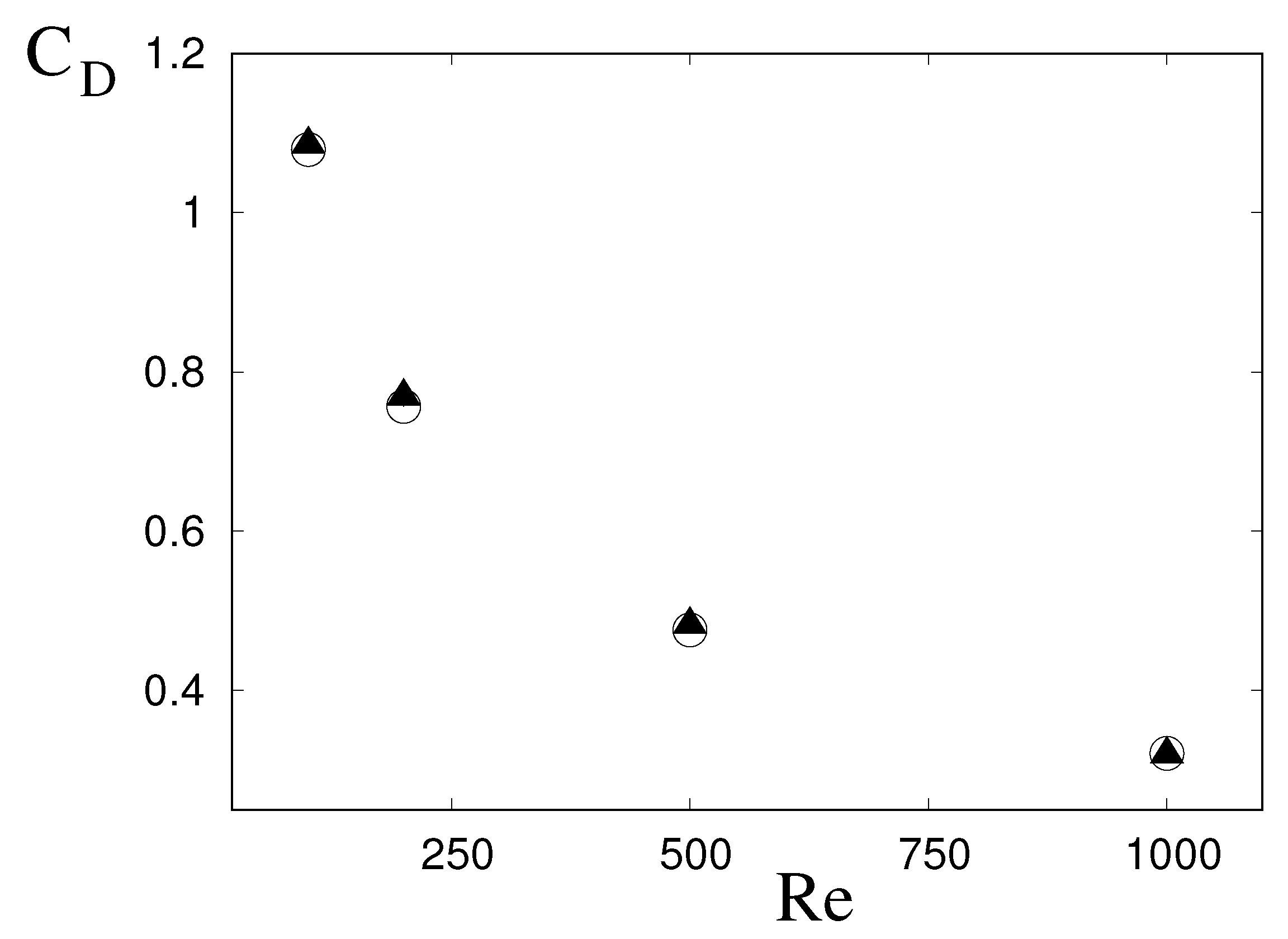
Figure 4.
Instantaneous snapshots of streamwise velocity (gray scales) and streamtraces ( ![Applsci 07 01108 i001]() ) for the flow around a torus at : (a) ; (b) ; (c) ; (d) ; (e) ; (f) .
) for the flow around a torus at : (a) ; (b) ; (c) ; (d) ; (e) ; (f) .
 ) for the flow around a torus at : (a) ; (b) ; (c) ; (d) ; (e) ; (f) .
Figure 4.
Instantaneous snapshots of streamwise velocity (gray scales) and streamtraces ( ![Applsci 07 01108 i001]() ) for the flow around a torus at : (a) ; (b) ; (c) ; (d) ; (e) ; (f) .
) for the flow around a torus at : (a) ; (b) ; (c) ; (d) ; (e) ; (f) .
) for the flow around a torus at : (a) ; (b) ; (c) ; (d) ; (e) ; (f) .
Figure 5.
Drag coefficient as function of the Reynolds number: (a) ∘ torus at , filled circular cylinder (data from [10] ┈ analytical expression with ; (b) ∘ torus at , ┈ line with . filled data for the same flow from [9].
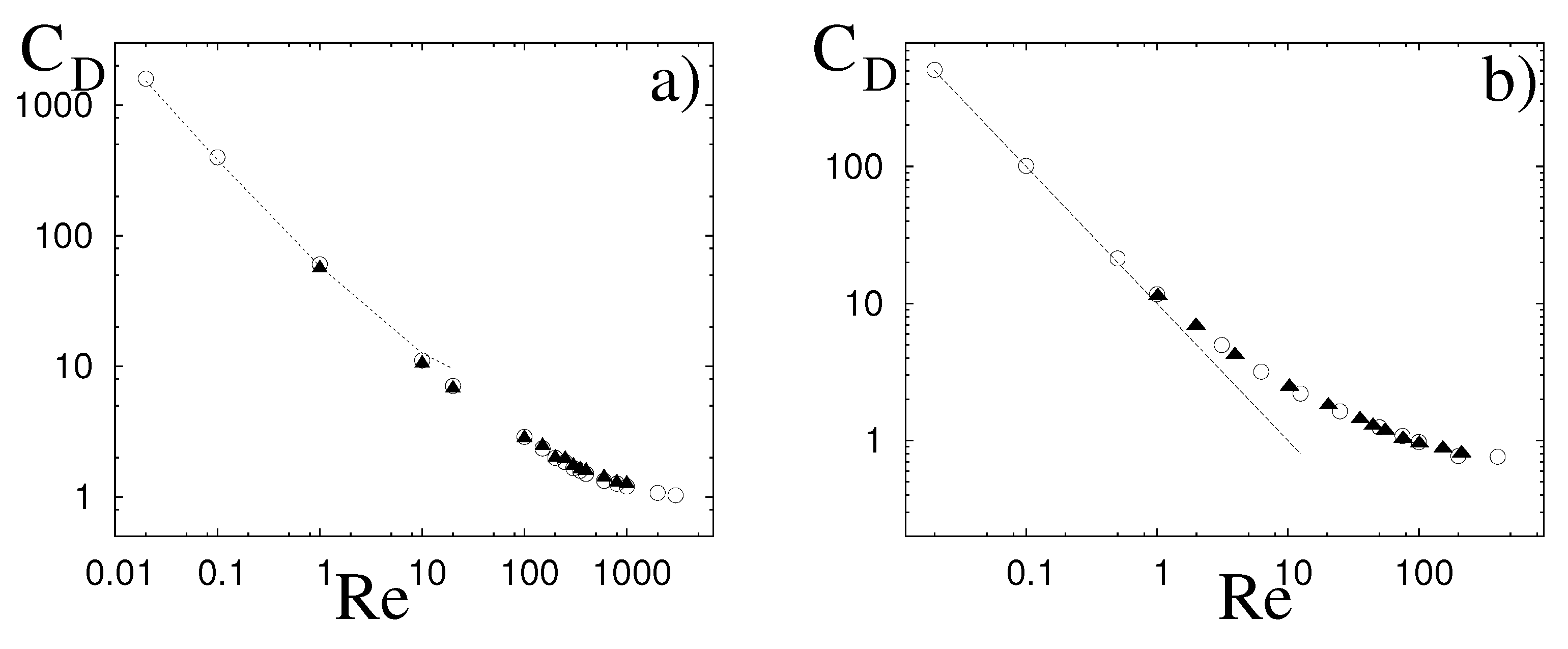
Figure 6.
Instantaneous snapshots of streamwise velocity (gray scales) and Stokes streamfunction ( ![Applsci 07 01108 i001]() for positive and ┈┈ for negative values) for the flow around a torus: (a) , ; (b) , ; (c) , ; (d) , .
for positive and ┈┈ for negative values) for the flow around a torus: (a) , ; (b) , ; (c) , ; (d) , .
for positive and ┈┈ for negative values) for the flow around a torus: (a) , ; (b) , ; (c) , ; (d) , .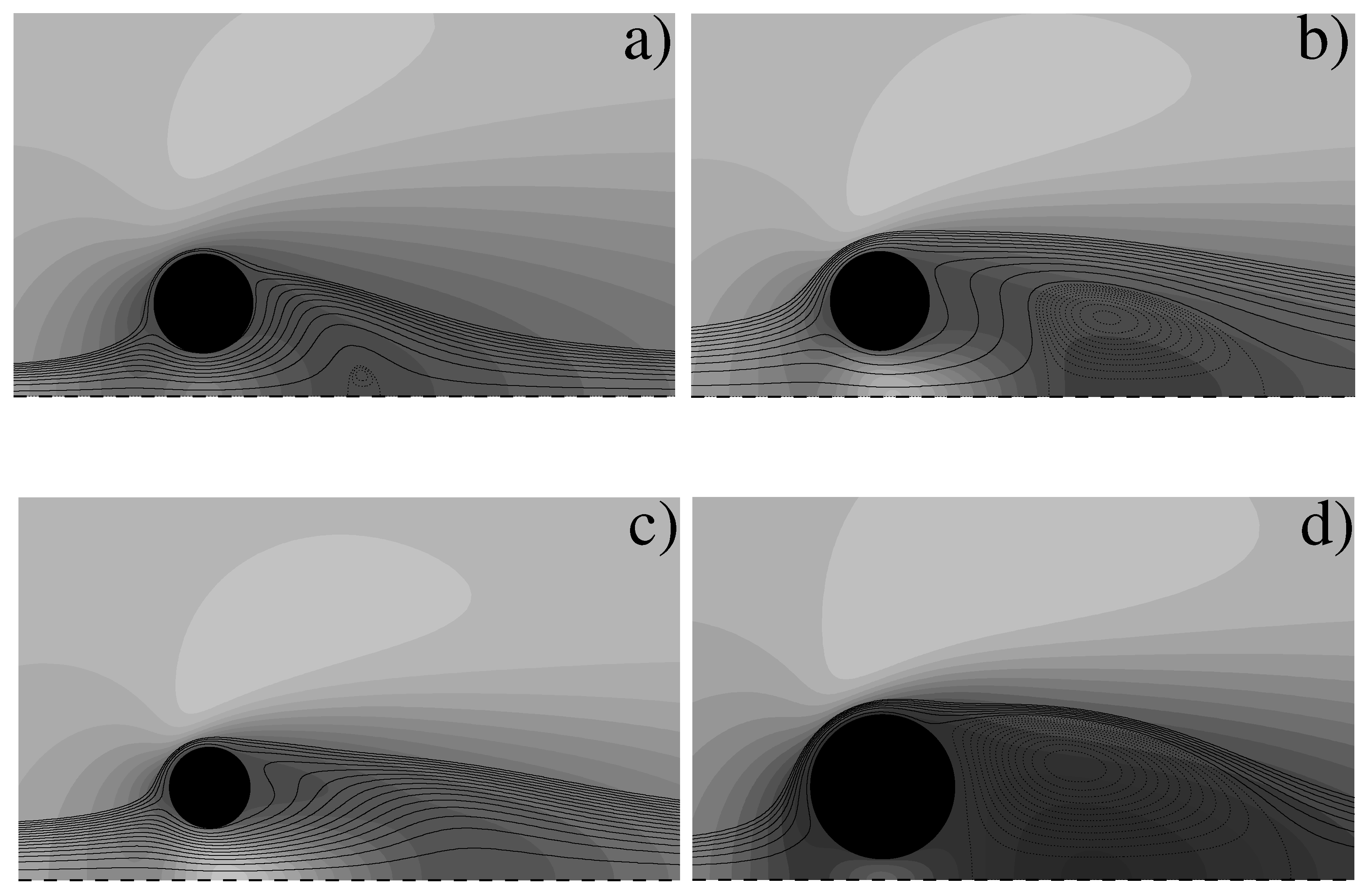
Figure 7.
Scatter plots of the azimuthal vorticity versus the radial coordinate r in the region of the recirculation bubble: (a) , ; (b) , .
Figure 7.
Scatter plots of the azimuthal vorticity versus the radial coordinate r in the region of the recirculation bubble: (a) , ; (b) , .

Figure 8.
(a) Stokes streamfunction as function of for the case at ; (b) as function of at .

Figure 9.
(a) Length of the separation bubble normalized by the core diameter versus Reynolds number: ∘ torus at , filled circular cylinder (from [10]). Instantaneous snapshots of streamwise velocity (gray scales) and Stokes streamfunction ( ![Applsci 07 01108 i001]() for positive ┈┈ for negative values); (b) , ; (c) , ; (d) , .
for positive ┈┈ for negative values); (b) , ; (c) , ; (d) , .
for positive ┈┈ for negative values); (b) , ; (c) , ; (d) , .
Figure 10.
Instantaneous snapshot of azimuthal vorticity (┈┈ for negative, ![Applsci 07 01108 i001]() for positive values) and Stokes streamfunction (﹊) for the flow around a torus at and . The dashed lines (┈┈) connect the centres of the vortices of the same sign.
for positive values) and Stokes streamfunction (﹊) for the flow around a torus at and . The dashed lines (┈┈) connect the centres of the vortices of the same sign.
for positive values) and Stokes streamfunction (﹊) for the flow around a torus at and . The dashed lines (┈┈) connect the centres of the vortices of the same sign.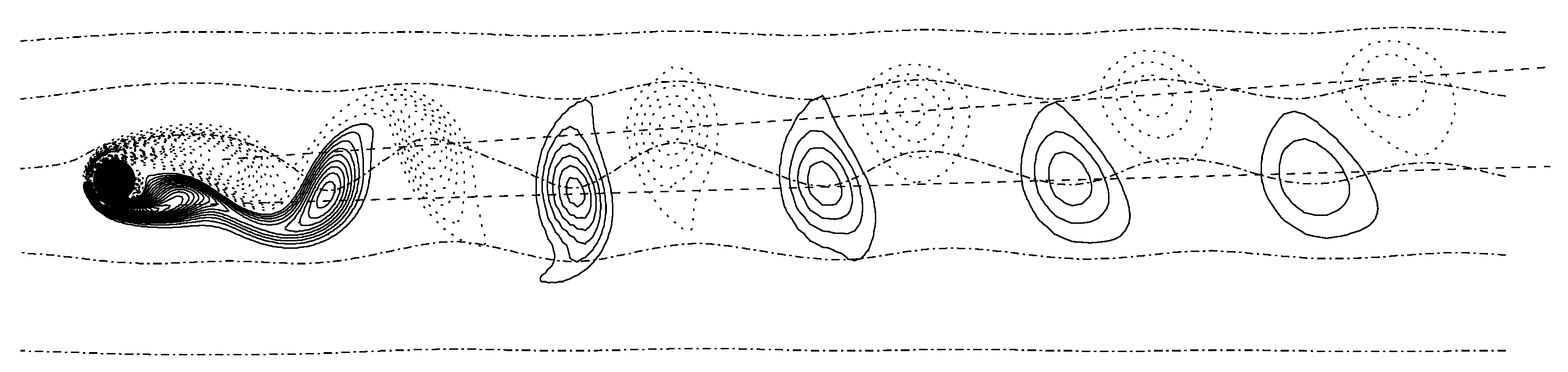
Figure 11.
(a) Time evolution of the drag coefficient for the flow at and (); (b) Strohual number () versus Reynolds number (): ![Applsci 07 01108 i001]() data for the circular cylinder (from [2]) ∘ flow around a torus at , flow around a torus at , • flow around a torus at .
data for the circular cylinder (from [2]) ∘ flow around a torus at , flow around a torus at , • flow around a torus at .
data for the circular cylinder (from [2]) ∘ flow around a torus at , flow around a torus at , • flow around a torus at .
Figure 12.
Instantaneous snapshots of streamwise velocity (gray scale) and streamtraces ( ![Applsci 07 01108 i001]() ) for the three-dimensional flow around a torus: (a) , ; (b) , .
) for the three-dimensional flow around a torus: (a) , ; (b) , .
) for the three-dimensional flow around a torus: (a) , ; (b) , .
© 2017 by the authors. Licensee MDPI, Basel, Switzerland. This article is an open access article distributed under the terms and conditions of the Creative Commons Attribution (CC BY) license (http://creativecommons.org/licenses/by/4.0/).
Share and Cite
MDPI and ACS Style
Lazeroms, W.M.J.; De Tullio, M.D.; De Santis, N.; Pizzoferrato, R.; Verzicco, R. Low Reynolds Number Flow Around Tori of Different Slenderness Γ. Appl. Sci. 2017, 7, 1108. https://doi.org/10.3390/app7111108
AMA Style
Lazeroms WMJ, De Tullio MD, De Santis N, Pizzoferrato R, Verzicco R. Low Reynolds Number Flow Around Tori of Different Slenderness Γ. Applied Sciences. 2017; 7(11):1108. https://doi.org/10.3390/app7111108
Chicago/Turabian StyleLazeroms, Werner M. J., Marco D. De Tullio, Nicola De Santis, Roberto Pizzoferrato, and Roberto Verzicco. 2017. "Low Reynolds Number Flow Around Tori of Different Slenderness Γ" Applied Sciences 7, no. 11: 1108. https://doi.org/10.3390/app7111108
Note that from the first issue of 2016, this journal uses article numbers instead of page numbers. See further details here.