Performance Evaluation of Submerged Floating Tunnel Subjected to Hydrodynamic and Seismic Excitations


Department of Civil and Environmental Engineering, Hanyang University, 222 Wangshimni-ro, Seoul 04763, Korea
*
Author to whom correspondence should be addressed.
Appl. Sci. 2017, 7(11), 1122; https://doi.org/10.3390/app7111122
Submission received: 24 September 2017
/
Accepted: 27 October 2017
/
Published: 31 October 2017
Abstract
:Submerged floating tunnels (SFTs) are innovative structural solutions to waterway crossings, such as sea-straits, fjords and lakes. As the width and depth of straits increase, the conventional structures such as cable-supported bridges, underground tunnels or immersed tunnels become uneconomical alternatives. For the realization of SFT, the structural response under extreme environmental conditions needs to be evaluated properly. This study evaluates the displacements and internal forces of SFT under hydrodynamic and three-dimensional seismic excitations to check the global performance of an SFT in order to conclude on the optimum design. The formulations incorporate modeling of ocean waves, currents and mooring cables. The SFT responses were evaluated using three different mooring cable arrangements to determine the stability of the mooring configuration, and the most promising configuration was then used for further investigations. A comparison of static, hydrodynamic and seismic response envelope curves of the SFT is provided to determine the dominant structural response. The study produces useful conclusions regarding the structural behavior of the SFT using a three-dimensional numerical model.
1. Introduction
Submerged floating tunnels (SFTs) are tubular structures that float at a specified depth and are supported by mooring cables. The balance between pre-tensions in the mooring cables and net positive buoyancy (or residual buoyancy) maintains the structural stability of the SFT. The cost of an SFT per unit length remains almost constant with increasing length [1,2]. Therefore, it is considered an economical alternative for waterway crossings in comparison to cable-supported bridges, underground tunnels or immersed tunnels, especially for deep and wide crossings. In addition, SFT is more advantageous, because it is not bound to geographic terrain and does not interfere with water surface traffic.
The research efforts for development of the SFT began in 1923 when the first Norwegian patent was issued for it. Since then, many case studies and proposals have been made for different proposed projects, such as Hogsfjord in Norway [3], Funka Bay in Japan [4,5], Messina Strait in Italy [6,7], Qiandao Lake in China [8,9] and Mokpo-Jeju SFT in South Korea [10].
The lack of experimental and model test results may be one of the reasons why an SFT has not yet been constructed. The work in [11] calculated the wave loads on a circular SFT using the boundary element method (BEM) and Morison’s equation and compared the results with model tests. Wave loads on an elliptical SFT were calculated similarly by [12] using Morison’s equation and compared with the test results. These studies indicated that both BEM and Morison’s equation gave reliable estimates of wave loads on SFT.
Researchers have focused the research developments on the behavior of SFT for more than three decades. A formulation for the dynamic analysis of the SFT under seismic and sea waves effects was presented by [13]. A primary attempt to analyze the fluid-structure interaction (FSI) of the SFT using a two-dimensional model was made by [14], followed by a more comprehensive presentation of FSI by [15] using the finite element implementation of the Navier–Stokes equation. The soil-structure interaction of SFT is another issue that needs to be investigated properly. Some SFT numerical models have idealized the soil-structure interaction as horizontal, vertical and rotational springs at the connecting points [16,17,18]. The vortex-induced vibrations of mooring cables caused by water currents can produce fatigue damage to the cables [19,20,21]. Since SFT is considered an alternative solution for transportation, moving load analysis or dynamic analysis under traffic loading is a key demand of the structure, but the research efforts are very limited regarding this problem. However, a primary attempt was made by [22], who investigated the effects of two- and three-dimensional added mass models on the response of SFT under single moving loads.
The numerical models described above focused on the dynamic response of SFT, including some recent developments [10,23,24]. However, the global performance of the SFT under complex environmental conditions is not yet well understood. The determination of stable mooring cable configurations for the SFT is one of the challenges for its realization [12,13]. Especially, the excessive lateral displacement of the SFT due to waves and currents make it questionable for safe transportation. Three different cable configurations were analyzed numerically by Mazzolani et al. [8] using the commercial software package ABAQUS/Aqua for the hydrodynamic conditions of Qiandao Lake (People’s Republic of China). Similar configurations are evaluated further in the present study for an SFT with a cable inclination of 45°, in order to check the performance of SFT. The mooring cables with this inclination are more stable [21,25]. In addition, a comparison of the SFT responses for static, hydrodynamic and seismic loadings needs to be provided for SFT performance quantification under different conditions.
More explicitly, this study evaluates the global performance of an SFT taking into account hydrodynamic and seismic excitations. The formulation of the problem includes the modeling of cable element, hydrodynamics, ground motions and the SFT structure itself. A numerical model of the SFT prototype to be built in Qindao Lake is used to evaluate the global performance under different loadings, and some useful conclusions are drawn that can provide an initial step towards the realization of this innovative structural solution for waterway crossings.
2. Governing Equations of Motion
2.1. Modeling of Waves and Currents
A schematic layout of the submerged floating tunnel (SFT) is shown in Figure 1. The X-, Y- and Z-axes are pointed along the axis of the tunnel, traverse and vertical to the tunnel axis, respectively. The tunnel is supported by vertical and inclined mooring cables.
Most of the wave theories used for the evaluation of wave forces on offshore structures are based on three parameters, i.e., water depth, wave height and wave period. The Airy wave theory, which holds for wave heights up to 10–15 m, covers a wide range and can consider significant waves of any actual sea states [13]. As the SFT is located at locations where the significant wave height is smaller than the water depth, the Airy wave theory can be used to model the sea states. According to the Airy wave theory, the first-order velocity potential is given as follows [26]:
where ; is the wave number; is the wave frequency; is the wavelength selected on the basis of deep-water criteria; is the wave height; is the wave speed; and are the vertical and transverse coordinates, respectively, having their origin at the free water surface; and is the water depth. From the first-order velocity potential , the water particle velocities in the transverse (Y) and vertical (Z) directions can be obtained as follows:
Differentiating the above equations with respect to time, the water particle accelerations in the transverse and vertical directions can be given as follows:
The calculation of hydrodynamic forces on the SFT is one of the primary tasks in the design of the structure. It is also one of the most challenging tasks during numerical simulations due to the involvement of the fluid-structure interaction phenomena [27]. Morison’s equation can be used to evaluate the hydrodynamic forces on the SFT and gives reliable estimates as compared to experimental data [11,12]. The hydrodynamic forces from ocean waves and currents, acting per unit length of the SFT, are given by the modified Morison’s equation as follows [26].
where subscript denotes the Y or Z direction; is the water particle velocity ( or ); is the water particle acceleration ( or ); is the velocity ( or ) of water currents acting at the centerline of the tunnel and is obtained by the linear equation: or ; and are the velocities of surface currents in the Y and Z directions, respectively. and are the structural velocity and acceleration, respectively; is the density of water; is the external diameter of SFT; is the drag coefficient; is the inertia coefficient; and is the added mass coefficient.
In Equation (6), the first term on the right-hand side denotes the drag force; the second term denotes the inertia force; and the third term denotes the added mass effect. The drag force is much smaller than the inertia [12], so the drag force term is linearized by removing the structural velocity term for numerical simplification. Substituting Equations (2)–(5) into Equation (6), the horizontal and vertical components of hydrodynamic forces in the Y-direction and the Z-direction can be obtained as follows:
where the subscripts YD and YI represent the fluid drag and inertia forces in the Y-direction respectively; the subscripts ZD and ZI represent the fluid drag and inertia forces in the Z-direction, respectively.
2.2. Equations of Motion
The equation of motion for the SFT moored by the mooring cables and subjected to gravity, hydrodynamic and seismic loads can be written in matrix form as follows:
where is the structural mass matrix of SFT; is the added mass matrix, which is the mass contribution by water and is obtained from the third term on the right hand side of Equation (6). is the system damping matrix. and are the elastic stiffness of the SFT and the mooring stiffness matrices, respectively. is the vector of time-dependent hydrodynamic forces. is the vector showing hydrostatic and live loads acting on the SFT. is the vector of ground motions acceleration. is the influence coefficient vector, having one for elements corresponding to the degrees of freedom in the direction of the applied ground motion and zero for the other degrees of freedom. , and are the vectors representing structural acceleration, velocity and displacement, respectively. The vector for an element is given as follows:
where , and are the displacements along the X, Y and Z directions, respectively; while and are the rotations about the Y-axis and Z-axis, respectively. The subscripts 1 and 2 represent the first and second nodes of an element, respectively.
The structural mass and the added mass are lumped at the nodes. The added mass is applied in the traverse and vertical directions only. The elastic stiffness is calculated using the 3D beam element, and the nonlinear mooring stiffness is calculated using the truss element. We used both cable elements and truss elements for modeling the mooring cables, and there was almost no difference in the response of the SFT due the fact that mooring cables always remain in tension under the input conditions of the present study. Therefore, we adopted the truss element. However, cable elements should be used in general when severe environmental conditions exist. In modeling the mooring cables, the residual buoyancy, which is the net hydrostatic force, was used as pretensions in the cable elements. The damping matrix is calculated using the Rayleigh damping model as follows:
where:
where and are the Rayleigh damping coefficients; is the modal damping ratio; and are the ith and jth modal natural frequencies of the structure, respectively. The mass and stiffness proportional Rayleigh damping coefficients are chosen based on the first two modes of SFT, so that the modal damping ratio is 2.5%. The same damping ratios have been used for the structure and for the cables due to the fact that SFT is a tubular structure and resembles a pipe [28].
The numerical procedure for the static and dynamic analysis is briefly described here. In the static analysis of SFT, the maximum wave and current forces were applied as uniformly-distributed static loads. In the dynamic analysis, the equations of motion were solved by Newmark’s direct time integration method. A computer program was developed to perform the dynamic analysis of SFT subjected to net residual buoyancy and time-dependent hydrodynamic and seismic forces. The tunnel was modeled using FEM with 30 3D-beam elements, and the torsional effect was neglected because it was very small.
3. Numerical Example
The performance evaluation of SFT needs to be carried out using a realistic model. Therefore, the prototype of the proposed SFT model, as shown in Figure 2 [8,9], which is planned to be built in Qiandao Lake, China, is evaluated in this study. The factored load combinations used by [8] were used for both static and hydrodynamic analyses in the present study.
Figure 2a shows the side view of the SFT model; the SFT is supported at Locations A, B and C by mooring cables. Figure 2b shows three different types of mooring cables arrangements. Figure 2c shows the material cross-section of the SFT. Three different SFT cases are analyzed based on three different mooring cable arrangements defined in Table 1, where the circled numbers represent the cable arrangement shown in Figure 2b. The input parameters for SFT tunnel, hydrodynamic and mooring cables are given in Table 2; the hydrodynamic parameters are those measured at Qindao Lake [8].
The assumptions made in this study and criteria are given as follows:
- The cross-section of the SFT is hollow circular, consisting of an external aluminum layer followed by a sandwiched concrete layer and internal steel layer. The material’s thicknesses and tunnel diameters are shown in Figure 2c. A uniformly-distributed load of 125 kN/m, per unit length, was used for the tunnel. The Archimedes buoyancy was 160 kN/m ( = 1050 × 10 × π × 4.42/4 = 160 kN/m), and the net residual buoyancy was 35 kN/m (160 − 125 = 35 kN/m). A uniformly-distributed live load of 10 kN/m was assumed to be acting on the tunnel;
- The mooring cable connections at the anchor point (seabed) and tunnel were treated as pins; and
- The tunnel displacements were restrained at one end, while the axial displacement was left free at the other end. The flexural rotations were allowed at both ends of the tunnel.
4. Results
4.1. Hydrodynamic Response
A comparative study of the SFT response using the three different cable configurations defined in Table 1 is presented. The configuration that proves to be the most promising is then used for further investigations.
The wave and current forces are obtained using the hydrodynamic conditions of Qiandao Lake (Table 2). These forces acting on the SFT are calculated using Morison’s equation. During the numerical simulations, the drag forces and inertia forces were considered distributed loadings and were converted to equivalent nodal forces using the work-equivalence method [29]. The time history of these forces per unit length of SFT is shown in Figure 3. The transverse and vertical inertia forces are dominant hydrodynamic forces, while the drag forces are very small.
4.1.1. Verification of the Numerical Model
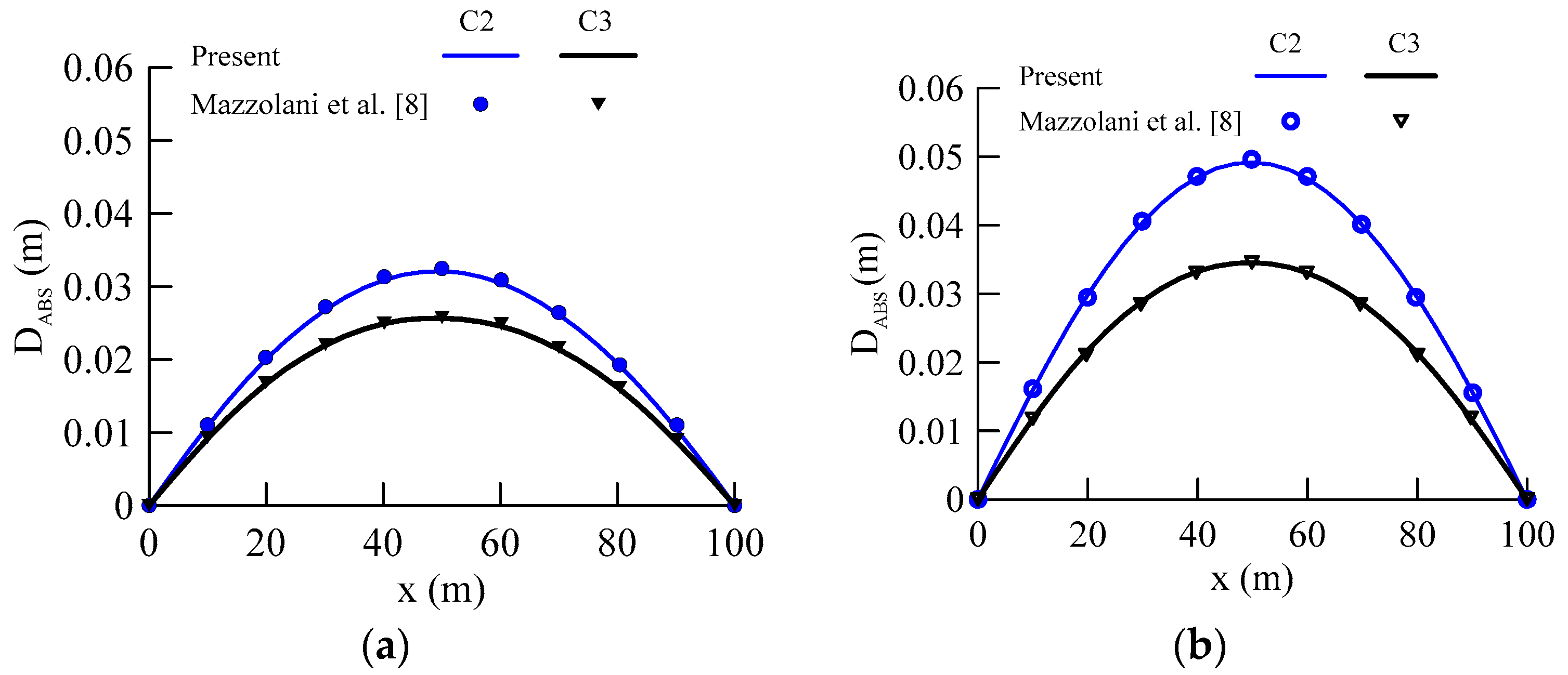
In order to verify the presented formulations and the numerical procedure, the static and dynamic responses of the SFT are compared with finite element results from ABAQUS/Aqua, Mazzolani et al. [8]. For comparison purposes, the absolute displacement is defined as follows:
where is the absolute displacement. The same definition is valid for both static and dynamic displacement. In the dynamic analysis, the maximum Y and Z displacements were used for calculating the absolute displacements.
Both static and dynamic absolute displacements based on the same input properties and cable configurations are compared with [8]. The comparisons of static and dynamic absolute displacements using mooring configurations C2 and C3 are shown in Figure 4a,b, respectively. The close agreement of the results shows the accuracy of the presented model.
4.1.2. Static Response
The maximum hydrodynamic forces in the transverse and vertical directions calculated from Equation (6) or (7) were applied as equivalent static nodal forces in the static analysis. The intensities of these forces in the transverse (Y) and vertical (Z) directions were 4.875 kN/m and 4.858 kN/m, respectively. The static analysis of the SFT is useful for assessing the performance of the SFT for the preliminary design.
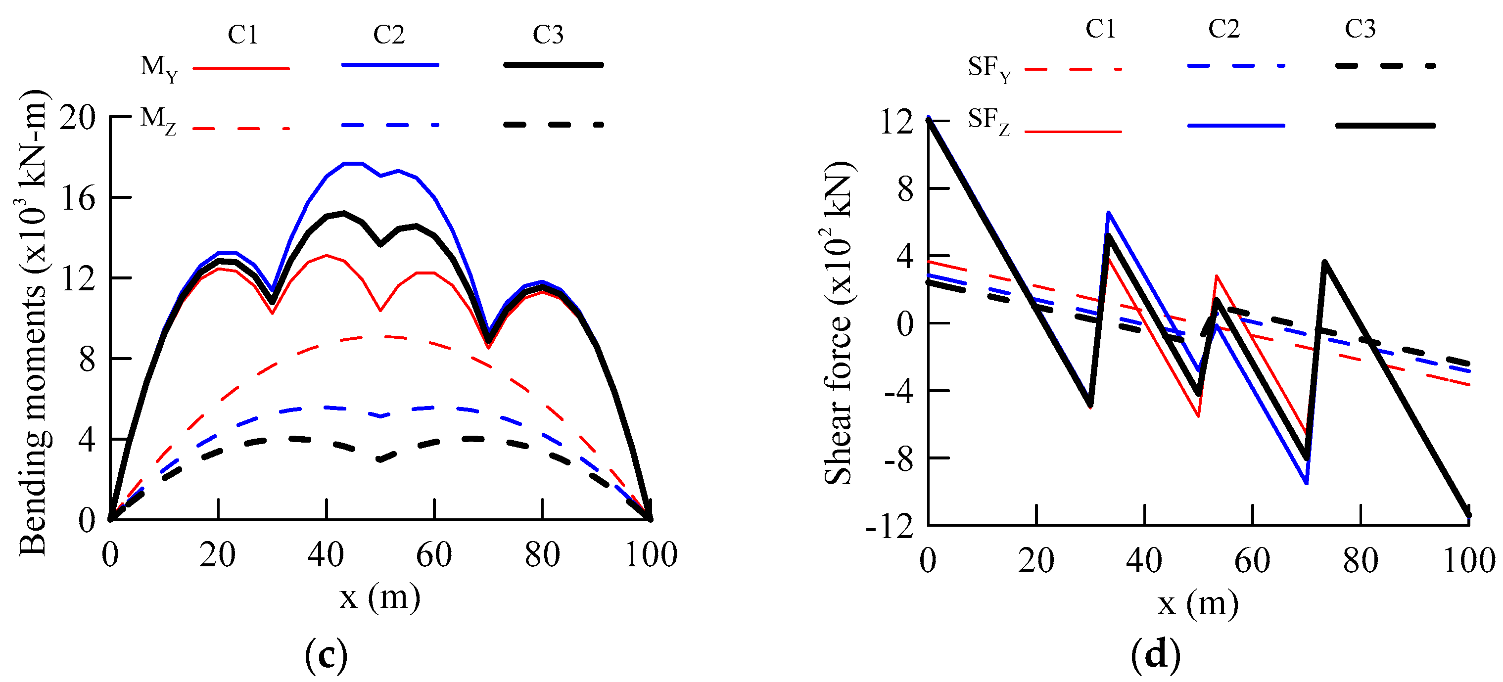
Static displacements and internal forces envelope curves of the SFT are shown in Figure 5. The transverse response of the SFT, i.e., rotations (), displacements (), bending moments (MZ) and shear forces (SFY) decreased when the mooring cable configuration was changed from C1 to C3. However, the vertical response, i.e., the rotations (), displacements (), bending moments (MY) and shear forces (SFZ), have different trends, where the response for configuration C2 is the greatest, followed by configuration C3, and configuration C1 has the minimum response. Comparisons of static displacements and internal forces of the SFT for three mooring configurations at Sections A, B and C (Figure 2a) are summarized in Table 3 to clearly show the trends described above.
The shape of bending moment gives direct insight into the cable configurations and performances of mooring systems and reflects the uniqueness of the adopted mooring cable configurations, as can be seen in Figure 5c. From these results, it can be concluded that the static response provides an important benchmark for decision-making regarding mooring cable arrangements and configuration selection for the preliminary design of SFT. However, the static response is very small and could not be used for the practical design of SFT, as shown in Figure 4, as will be demonstrated further in the following sections.
4.1.3. Dynamic Response
The modal analysis was performed, and the natural frequencies of the first 20 natural modes are listed in Table 4. The comparison of the natural frequencies of the SFT supported by different mooring cable configurations gives a direct measure of the cable system stiffness. The natural frequencies of the SFT increase when the cable configuration is changed from C1 to C3. Configuration C3 provides more stiffness to the SFT than configurations C1 and C2, and similarly, configuration C2 provides more than configuration C1. However, the natural frequencies of the SFT for the three mooring cable configurations are very close to each other for higher modes.
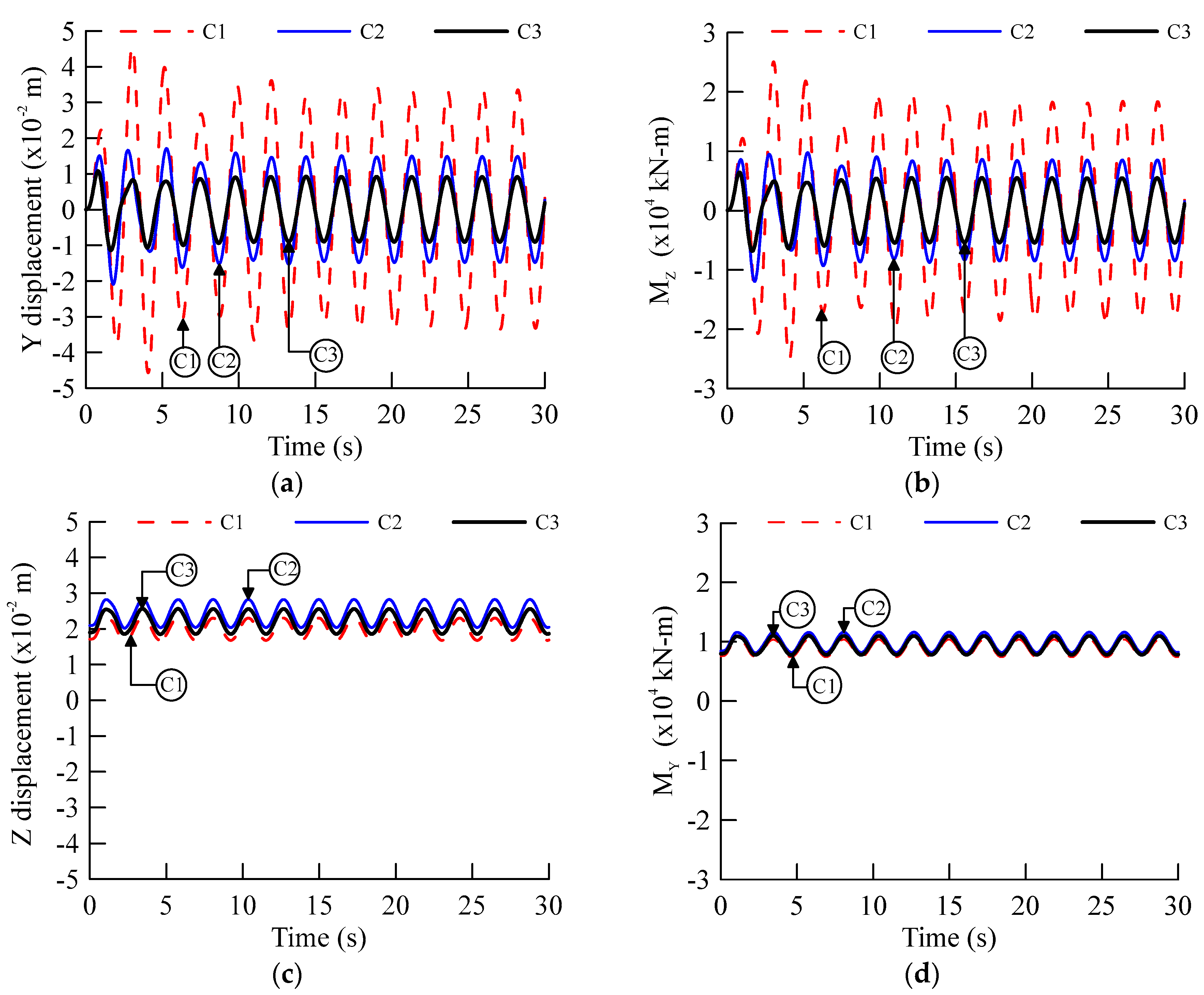
Figure 6 represents the comparison of the hydrodynamic response of the SFT at Section A, using three mooring cable configurations. Figure 6a shows the comparison of the SFT displacements in the transverse direction: configuration C1 has the largest displacement, followed by configuration C2, and configuration C3 has the minimum displacement. The maximum displacements of the SFT for configuration C1, C2 and C3 are 0.046 m, 0.021 m and 0.011 m, respectively. The same trend occurs for the transverse bending moment (Mz), as shown in Figure 6b. The maximum bending moments of SFT for configurations C1, C2 and C3 are 25,066.628 kN-m, 11,943.442 kN-m and 6838.661 kN-m, respectively. Figure 6c shows the comparison of the SFT displacement in the vertical direction; configuration C2 has the largest displacement, followed by configuration C3, and configuration C1 has the minimum displacement. The maximum displacements of SFT for configurations C1, C2 and C3 are 0.029 m, 0.035 m and 0.032 m, respectively. The same trend occurs for the vertical bending moment (MY), as shown in Figure 6d. The maximum bending moments of SFT for configurations C1, C2 and C3 are 12,202.859 kN-m, 13,694.792 kN-m and 12,934.200 kN-m, respectively.
Figure 7 represents the comparison of the hydrodynamic response of SFT at Section B. Figure 7 shows the same trend as described to that of Section A. However, the general response at Section B is larger than that of Section A. In addition, the response shown by configuration C3 here is further reduced as compared to Section A, because Section B is supported by double inclined mooring cables.
Both Figure 6 and Figure 7 show that the transient motions of the SFT are small and decay quickly with time, and the steady-state motions are more pronounced, especially in the traverse direction, as is clear from the Y-displacement and bending moment MZ. In the vertical direction, the SFT vibrated under the effect of inertial force and buoyancy force like a beam on elastic supports, as shown by the Z-displacement and bending moment MY in Figure 6c,d and Figure 7c,d, respectively. The SFT moored by tension leg mooring cables (C1) showed high peaks in the displacements and bending moments. The SFT moored by a tension leg and a single inclined mooring cable at the center (C2) provided better stiffness in the transverse direction, but lesser stiffness in the vertical direction. The SFT moored by double inclined mooring cables at the center (C3) showed the minimum response in the transverse direction. The response of SFT moored by the C1 and C2 configurations showed large peaks, due to very small restraining in the transverse direction. Therefore, C3 type configurations should be used at one or more locations at least, depending on the overall length of the SFT. It can be concluded that the C3 type cable configuration is more stable.
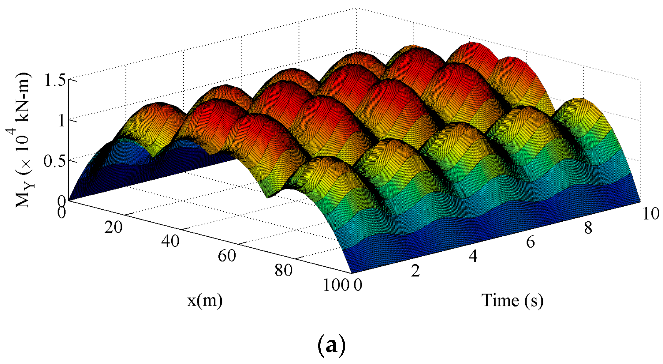
The SFT moored by mooring cable configuration C3 is used for the analysis hereafter. Three-dimensional visualization of the SFT response in both time and space gives a very clear understating of the structural behavior of the SFT subjected to hydrodynamic waves and currents. The three-dimensional time histories of the displacements and bending moments are shown in Figure 8 and Figure 9. The response of the SFT is plotted along the Z-axis; the tunnel longitudinal coordinates (x) are plotted along the X-axis; and time is plotted along the Y-axis.
Figure 8 show the displacements along the length of the tunnel with time. Figure 8a illustrates that the SFT vibrates harmonically in the Y-direction both in the positive and negative extremities.
Figure 8b also shows a harmonic motion pattern, but only in the positive limit (this upward positive displacement is caused by the residual buoyancy acting on the SFT in this direction); which means that the cables were in taut conditions and did not permit slackness in this direction.
Figure 9a shows the bending moment MY distribution along the length of the tunnel with time. The shape of bending moments gives a clear picture of the mooring cables configuration (C3) used. The inclined mooring cables at the central location provided flexible elastic bilateral restraint to the transverse and almost unilateral restraint to the vertical motion.
Figure 9b shows the bending moment MZ distribution along the length of the tunnel with time, and it is similar to the one related to a uniform beam vibrating in the first natural mode. It can be seen that only inclined cables, located at the center, provided significant restraining in the transverse direction (i.e., MZ), and the other two groups of vertical cables from left and right of the center provided almost no restraining in the transverse direction.
4.2. Seismic Response
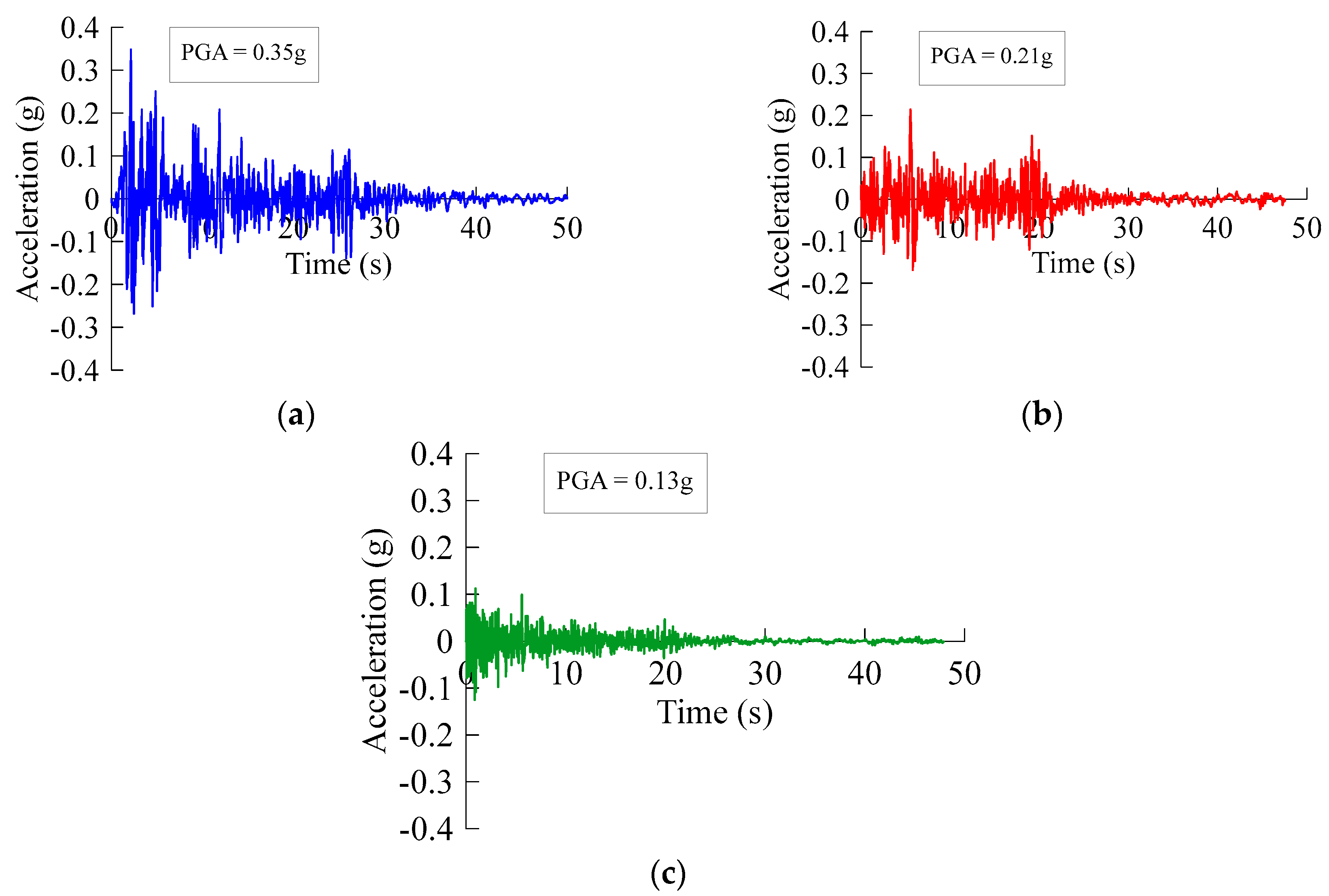
As stated before, the SFT is a massive tubular structure, and its structural response dramatically increases with external forcing. To check the maximum or dominant structural response of SFT, a comparison of static, hydrodynamic and seismic response needs to be provided [16,23]. The El-Centro (1940) ground motions are assumed for the SFT numerical example to evaluate the dynamic behavior of the SFT for the three-dimensional ground motion input. Three components of El-Centro ground motions used as input motions are shown in Figure 10. The effective seismic forces using these ground motions are applied simultaneously at the nodal points in the three-dimensional numerical model.
For the evaluation of the ground motion’s effects on the structural behavior of the SFT, two cases are defined: Case (1): The ground motion component S00E was applied in the longitudinal direction (X-direction); component S90W was applied in the transverse; and the vertical component was applied in the vertical direction of the SFT, respectively; this case will be referred to as Load Combination 1 (LC1). Case (2): The ground motion component S90W was applied in the longitudinal direction; component S00E was applied in the transverse direction; the vertical component was applied in the vertical direction of the SFT, respectively; this case will be referred to as Load Combination 2 (LC2). The ground motion component S00W is the maximum ground motion input having a peak ground acceleration (PGA) of 0.35 g. In contrast with the previous sections, the unfactored static and hydrodynamic loads are used here for evaluating the structural behavior of the SFT.
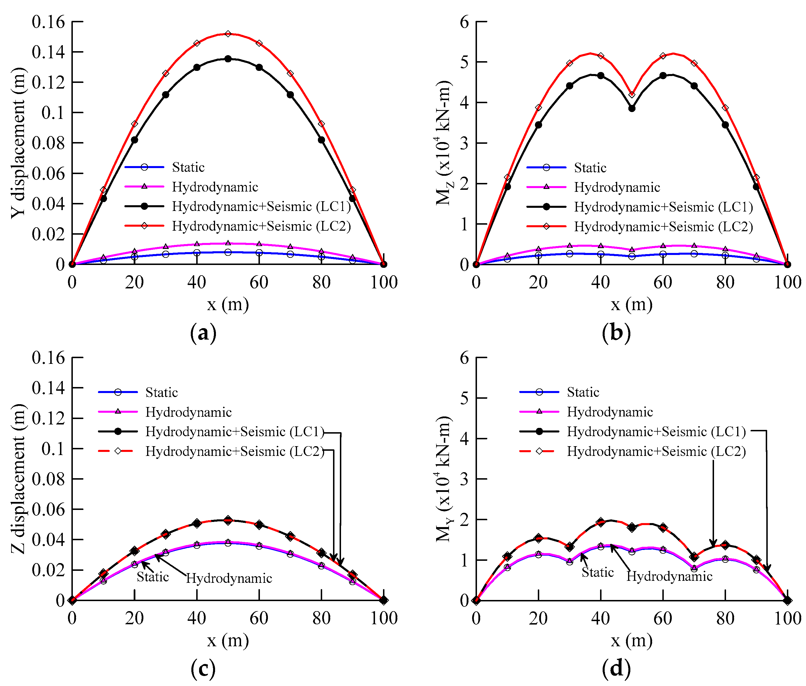
A comparison of the static, hydrodynamic and seismic response envelope curves of the SFT is shown in Figure 11. The maximum response of the tunnel is used to produce the envelope curves. The SFT response envelope curves of transverse and vertical displacements are shown in Figure 11a,b respectively; the longitudinal response of the SFT is very small and is not shown.
The transverse displacements of SFT in Figure 11a show a large difference between the static and dynamic analysis. The approximate relative differences in maximum transverse displacements of the SFT from analysis cases LC2, LC1 and hydrodynamics to that of the static case are 95%, 94% and 42%, respectively.
The vertical displacements of the SFT are nearly the same for static and hydrodynamic analysis. Similarly, for LC1 and LC2, the vertical displacements of the SFT are almost the same, as shown in Figure 11c. The approximate relative differences in maximum vertical displacements of the SFT from analysis cases LC2, LC1 and hydrodynamics to that of the static case are 28%, 28% and 1.7%, respectively.
The transverse response is more affected by the ground motions, while the vertical response is more affected by gravity and hydrodynamic (waves and currents) actions. The transverse response is extremely large for the seismic analysis as compared to the vertical response; for instance, the relative difference in transverse and vertical displacements for LC1 and LC2 are 61% and 65%, respectively.
Figure 11b,d represents the SFT bending moment MZ and bending moment MY envelope curves, respectively. Similar trends prevail for bending moments as described for displacements. The shape of bending moments clearly demonstrates the effectiveness of the adopted mooring configuration.
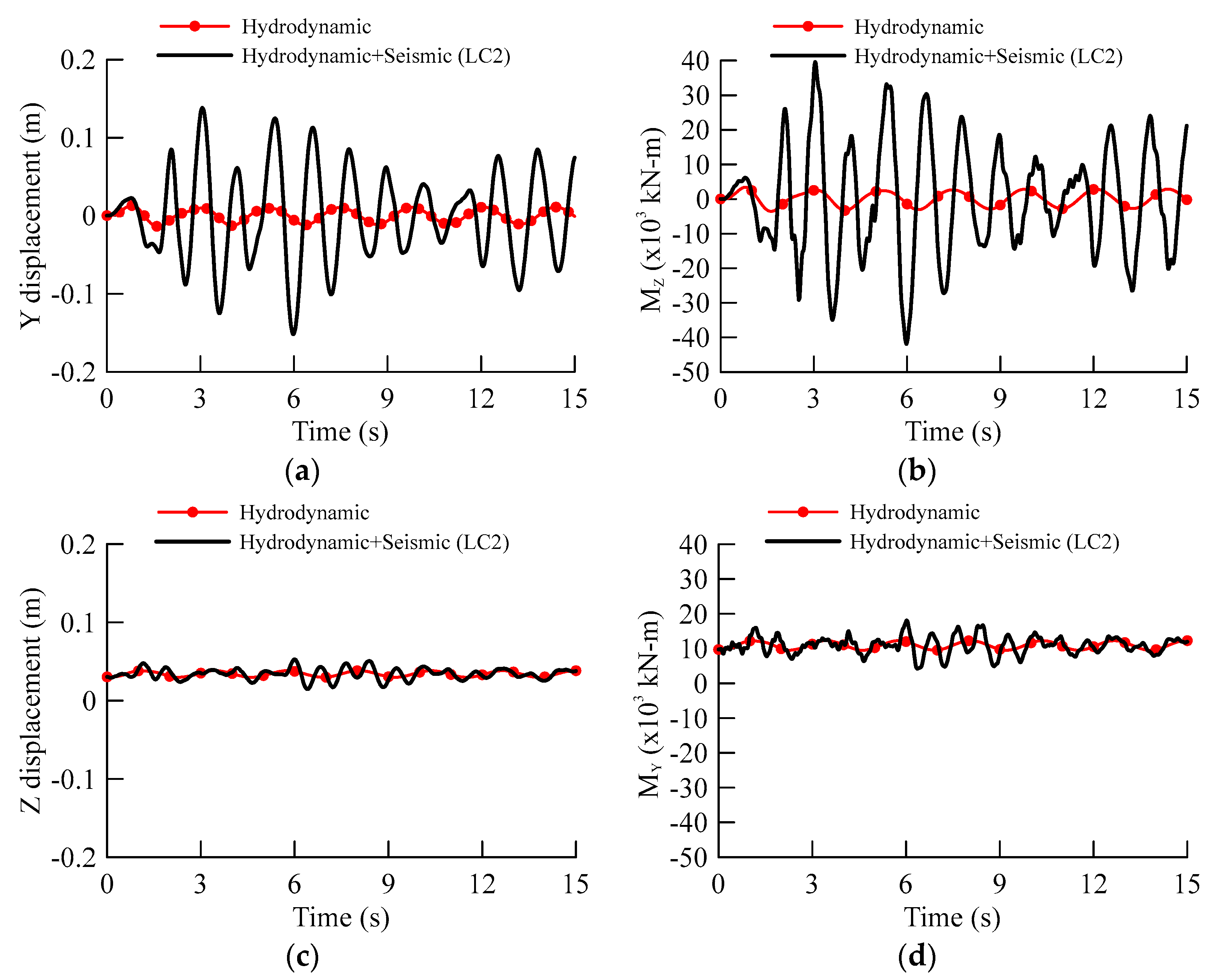
To show a clear picture of the dynamic response of the SFT under seismic loadings, the comparison of mid-span displacements and bending moments for hydrodynamic and seismic analysis (LC2) are shown in Figure 12. The hydrodynamic response is very small as compared to when the seismic load is considered. The comparison is shown only for one seismic scenario (LC2); due to that, both seismic load combinations (LC1, LC2) produce very close responses in comparison to hydrodynamic analysis. The hydrodynamic response of the SFT resembles the shape of the wave force model used, while the seismic loading effect the transient motion of the SFT. In addition, the transverse displacements (Figure 12a) and transverse bending moment (MZ, Figure 12b) are very large and significantly affected by seismic loading as compared to vertical displacements (Figure 12c) and vertical bending moment (MY, Figure 12d), and this is attributed to the small cable stiffness in the transverse direction.
5. Conclusions
The submerged floating tunnel (SFT) is a new structural solution to waterway crossings. Despite some valuable research having been accomplished, no SFT has been constructed in the world up to now. For the realization of SFT projects, the global performance in extreme environmental conditions needs to be properly evaluated. This study evaluates the displacements and internal forces of an SFT subjected to hydrodynamic and seismic loadings. The SFT tunnel was modeled by 3D beam elements; the mooring cables were modeled by truss elements; the ocean waves and currents were modeled by Airy wave theory. The SFT response subjected to hydrodynamic loading was evaluated using three different mooring cable configurations; the suitable mooring cable configuration was then used for further evaluation. A comparison of response envelope curves for static, hydrodynamic and seismic loadings was presented to evaluate the most effective structural response of SFT.
Based on the present study, the following conclusions can be drawn:
- The static response can provide a benchmark for decision-making on mooring cable arrangements and configurations for the preliminary design. However, the static analysis underestimates the responses in comparison to those of dynamic analysis
- The SFT moored by tension leg mooring cables was least effective, because of lesser horizontal stiffness, and the SFT moored by such mooring cables undergoes extreme displacements in the transverse direction as compared to the one moored by inclined mooring cables. The SFT moored by a combination of tension legs and single inclined mooring cables was effective for moderate environmental conditions. For severe environmental conditions, the SFT should be moored either by a combination of tension legs and double inclined mooring cables or only by double inclined mooring cables.
- For hydrodynamic analysis, the transient motions of SFT were small and decayed quickly, and the steady-state motions mainly governed the structural response of SFT under the prescribed damping conditions. In the case of the seismic analysis, the transient motions are more pronounced as compared to the hydrodynamic response.
- In the hydrodynamic analysis, the vertical response of SFT was very small and mainly attributed to gravity and hydrodynamic forces; while the transverse response was very large for seismic analysis. The transverse displacements and internal forces were found to be larger than those of the vertical direction, which showed less restraining and lesser mooring cable stiffness in the transverse direction.
Acknowledgments
The Basic Science Research Program through the National Research Foundation of Korea (NRF), funded by the Ministry of Education, Science and Technology (NRF-2015R1D1A1A09060113), supported this research. The authors wish to express their gratitude for this financial support.
Author Contributions
Dong-Ho Choi supervised the research. Naik Muhammad contributed the idea, performed the numerical simulations and wrote the manuscript. Zahid Ullah helped with the simulations and the writing of the manuscript.
Conflicts of Interest
The authors declare no conflict of interest.
References
- Ahrens, D. Chapter 10 submerged floating tunnels—A concept whose time has arrived. Tunn. Undergr. Space Technol. 1997, 12, 317–336. [Google Scholar] [CrossRef]
- Faggiano, B.; Landolfo, R.; Mazzolani, F. The SFT: An innovative solution for waterway strait crossings. IABSE Symp. Rep. 2005, 90, 36–42. [Google Scholar] [CrossRef]
- Skorpa, L. Innovative Norwegian fjord crossing. How to cross the HØGSJORD, alternative methods. In Proceedings of the 2nd Congress AIOM (Marine and Offshore Engineering Association), Naples, Italy, 15–17 November 1989. [Google Scholar]
- Maeda, N.; Morikawa, M.; Ishikawa, K.; Kakuta, Y. Study on structural characteristics of support systems for submerged floating tunnel. In Proceedings of the 3rd Symposium on Strait Crossings, Ålesund, Norway, 12–15 June 1994; pp. 579–674. [Google Scholar]
- Lu, W.; Ge, F.; Wang, L.; Wu, X.; Hong, Y. On the slack phenomena and snap force in tethers of submerged floating tunnels under wave conditions. Mar. Struct. 2011, 24, 358–376. [Google Scholar] [CrossRef]
- Bruschi, R.; Giardinieri, V.; Marazza, R.; Merletti, T. Submerged Buoyant Anchored Tunnels: Technical Solution for the Fixed Link across the Strait of Messina Strait Crossings; Balkema: Rotterdam, Dutch, 1990. [Google Scholar]
- Faggiano, B.; Landolfo, R.; Mazzolani, F. Design and modelling aspects concerning the submerged floating tunnels: An application to the Messina strait crossing. In Proceedings of the Fourth Symposium on Strait Crossings, Bergen, Norway, 2–5 September 2001; pp. 1–5. [Google Scholar]
- Mazzolani, F.; Landolfo, R.; Faggiano, B.; Esposto, M.; Perotti, F.; Barbella, G. Structural analyses of the submerged floating tunnel prototype in Qiandao Lake (PR of China). Adv. Struct. Eng. 2008, 11, 439–454. [Google Scholar] [CrossRef]
- Martinelli, L.; Barbella, G.; Feriani, A. A numerical procedure for simulating the multi-support seismic response of submerged floating tunnels anchored by cables. Eng. Struct. 2011, 33, 2850–2860. [Google Scholar] [CrossRef]
- Han, J.S.; Won, B.; Park, W.-S.; Ko, J.H. Transient response analysis by model order reduction of a Mokpo-Jeju submerged floating tunnel under seismic excitations. Struct. Eng. Mech. 2016, 57, 921–936. [Google Scholar] [CrossRef]
- Kunisu, H. Evaluation of wave force acting on submerged floating tunnels. Procedia Eng. 2010, 4, 99–105. [Google Scholar] [CrossRef]
- Seo, S.I.; Mun, H.S.; Lee, J.H.; Kim, J.H. Simplified analysis for estimation of the behavior of a submerged floating tunnel in waves and experimental verification. Mar. Struct. 2015, 44, 142–158. [Google Scholar] [CrossRef]
- Brancaleoni, F.; Castellani, A.; D’Asdia, P. The response of submerged tunnels to their environment. Eng. Struct. 1989, 11, 47–56. [Google Scholar] [CrossRef]
- Okstad, K.M.; Haukas, T.; Remseth, S.; Mathisen, K.M. Fluid-structure interaction simulation of submerged floating tunnels. In Computational Mechanics New Treds and Applications; Centro Internacional de Métodos Numéricos en Ingeniería: Barcelona, Spain, 1998; pp. 1–13. [Google Scholar]
- Remseth, S.; Leira, B.J.; Okstad, K.M.; Mathisen, K.M.; Haukås, T. Dynamic response and fluid/structure interaction of submerged floating tunnels. Comput. Struct. 1999, 72, 659–685. [Google Scholar] [CrossRef]
- Di Pilato, M.; Perotti, F.; Fogazzi, P. 3D dynamic response of submerged floating tunnels under seismic and hydrodynamic excitation. Eng. Struct. 2008, 30, 268–281. [Google Scholar] [CrossRef]
- Di Pilato, M.; Feriani, A.; Perotti, F. Numerical models for the dynamic response of submerged floating tunnels under seismic loading. Earthq. Eng. Struct. Dyn. 2008, 37, 1203–1222. [Google Scholar] [CrossRef]
- Fogazzi, P.; Perotti, F. The dynamic response of seabed anchored floating tunnels under seismic excitation. Earthq. Eng. Struct. Dyn. 2000, 29, 273–295. [Google Scholar] [CrossRef]
- Li, J.; Li, Y. Analytical solution to the vortex-excited vibration of tether in the submerged floating tunnel. Am. Soc. Civ. Eng. 2006, 164–169. [Google Scholar] [CrossRef]
- Luoa, G.; Chen, J.; Zhou, X. Effects of various factors on the viv-induced fatigue damage in the cable of submerged floating tunnel. Pol. Marit. Res. 2015, 22, 76–83. [Google Scholar] [CrossRef]
- Yiqiang, X.; Chunfeng, C. Vortex-induced dynamic response analysis for the submerged floating tunnel system under the effect of currents. J. Waterw. Port Coast. Ocean Eng. 2012, 139, 183–189. [Google Scholar] [CrossRef]
- Tariverdilo, S.; Mirzapour, J.; Shahmardani, M.; Shabani, R.; Gheyretmand, C. Vibration of submerged floating tunnels due to moving loads. Appl. Math. Model. 2011, 35, 5413–5425. [Google Scholar] [CrossRef]
- Lee, J.H.; Seo, S.I.; Mun, H.S. Seismic behaviors of a floating submerged tunnel with a rectangular cross-section. Ocean Eng. 2016, 127, 32–47. [Google Scholar] [CrossRef]
- Mirzapour, J.; Shahmardani, M.; Tariverdilo, S. Seismic response of submerged floating tunnel under support excitation. Ships Offshore Struct. 2016, 1–8. [Google Scholar] [CrossRef]
- Xiang, Y.; Yang, Y. Spatial dynamic response of submerged floating tunnel under impact load. Mar. Struct. 2017, 53, 20–31. [Google Scholar] [CrossRef]
- Chakrabarti, S.K. Hydrodynamics of Offshore Structures; WIT Press: Southampton, UK, 1987. [Google Scholar]
- Sarpkaya, T.; Isaacson, M. Mechanics of Wave Forces on Offshore Structures; Van Nostrand Reinhold: New York, NY, USA, 1981. [Google Scholar]
- Veritas, D.N. Free Spanning Pipelines; Recommended Practice DNV-RPF105; Det Norske Veritas Germanischer Lloyd (DNV GL): Oslo, Norway, 2006; Available online: http://rules.dnvgl.com/docs/pdf/DNV/codes/docs/2006-02/RP-F105.pdf (accessed on 24 September 2017).
- Logan, D.L. A First Course in the Finite Element Method; Cengage Learning: Boston, MA, USA, 2011. [Google Scholar]
Figure 1.
Schematic layout of the submerged floating tunnel (SFT): (a) side view of the SFT and (b) cross-sectional view of the SFT.
Figure 1.
Schematic layout of the submerged floating tunnel (SFT): (a) side view of the SFT and (b) cross-sectional view of the SFT.
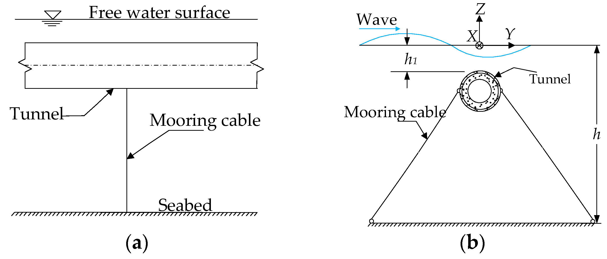
Figure 2.
Schematic layout of the submerged floating tunnel (SFT): (a) side view of the SFT and (b) mooring cables arrangements; and (c) material cross-section of the SFT.
Figure 2.
Schematic layout of the submerged floating tunnel (SFT): (a) side view of the SFT and (b) mooring cables arrangements; and (c) material cross-section of the SFT.
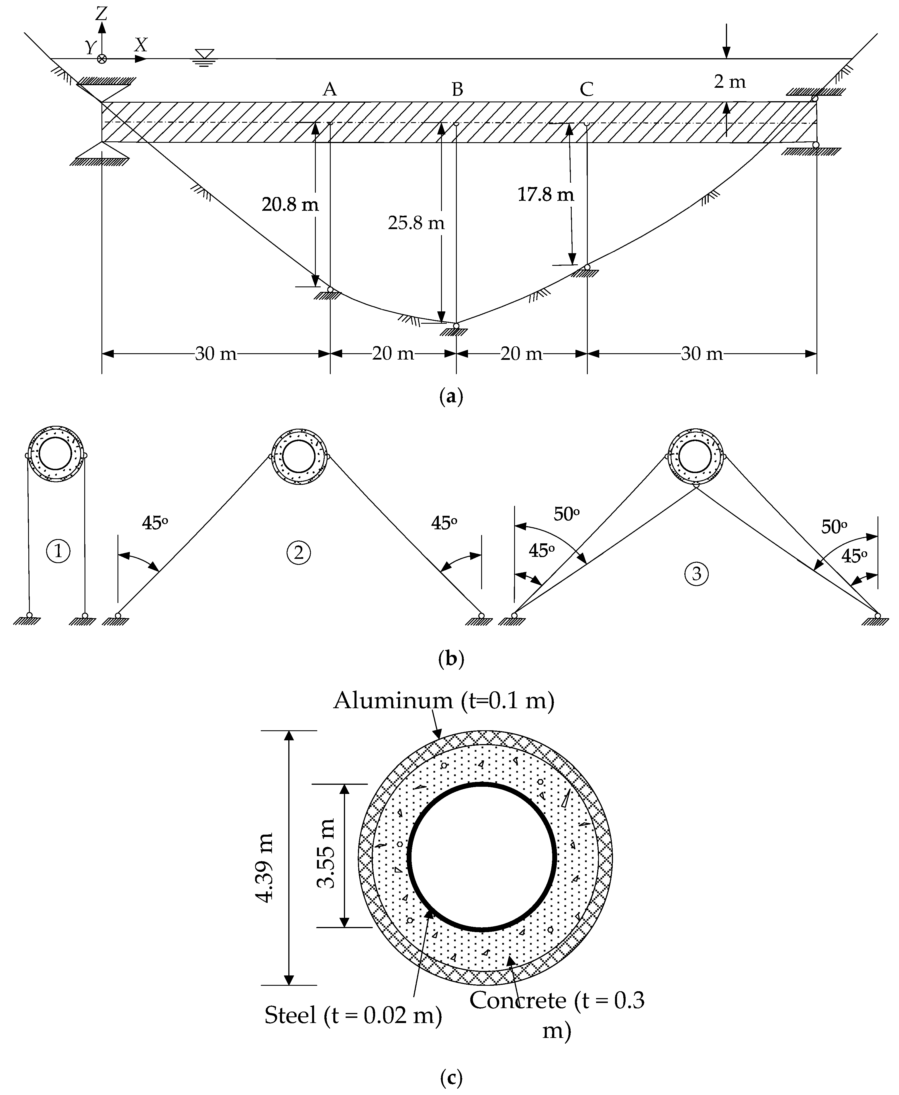
Figure 3.
Hydrodynamic force time history per unit length of the SFT.
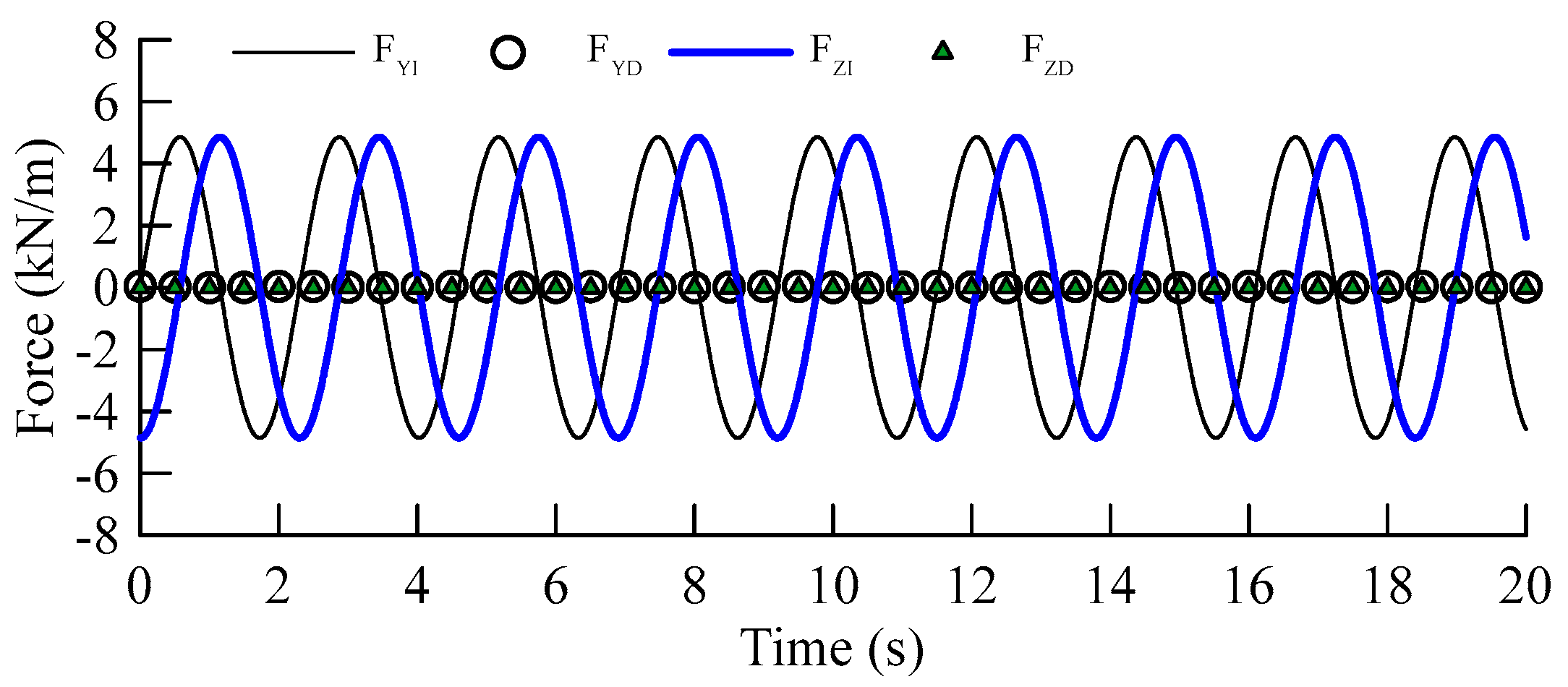
Figure 4.
Comparison of absolute displacements with ABAQUS/Aqua [8]: (a) absolute static displacement and (b) absolute dynamic displacement.
Figure 4.
Comparison of absolute displacements with ABAQUS/Aqua [8]: (a) absolute static displacement and (b) absolute dynamic displacement.

Figure 5.
Comparison of static displacement and internal force envelope curves of the SFT for three mooring configurations: (a) vertical and transverse rotation; (b) vertical and transverse displacement; (c) vertical and transverse bending moment; and (d) vertical and transverse shear force.
Figure 5.
Comparison of static displacement and internal force envelope curves of the SFT for three mooring configurations: (a) vertical and transverse rotation; (b) vertical and transverse displacement; (c) vertical and transverse bending moment; and (d) vertical and transverse shear force.
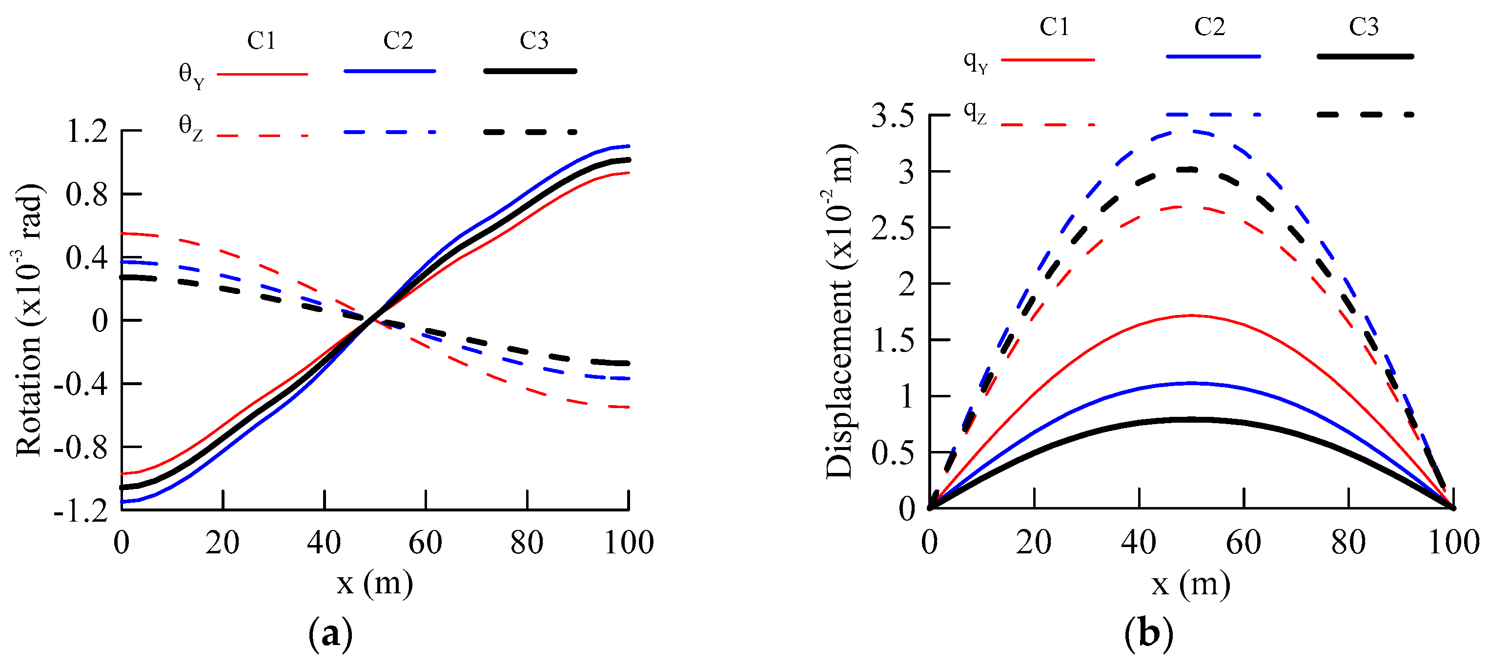

Figure 6.
Comparison of the hydrodynamic response of the SFT at Section A: (a) Y-displacement; (b) bending moment MZ; (c) Z-displacement; and (d) bending moment MY.
Figure 6.
Comparison of the hydrodynamic response of the SFT at Section A: (a) Y-displacement; (b) bending moment MZ; (c) Z-displacement; and (d) bending moment MY.

Figure 7.
Comparison of the hydrodynamic response of the SFT at Section B: (a) Y-displacement; (b) bending moment MZ; (c) Z-displacement; and (d) bending moment MY.
Figure 7.
Comparison of the hydrodynamic response of the SFT at Section B: (a) Y-displacement; (b) bending moment MZ; (c) Z-displacement; and (d) bending moment MY.
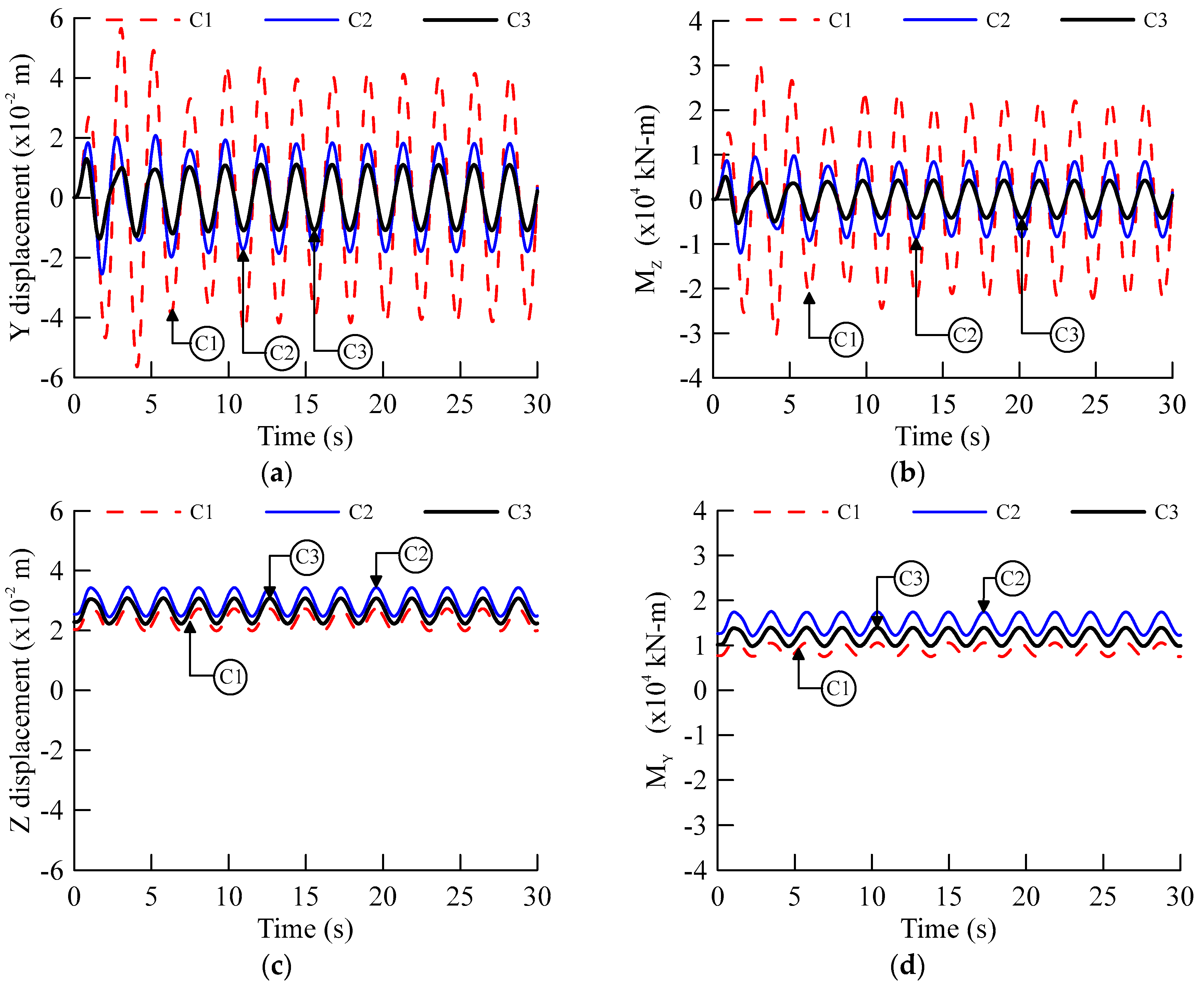
Figure 8.
Hydrodynamic displacements along the length of the SFT with time: (a) Y-displacement and (b) Z-displacement.
Figure 8.
Hydrodynamic displacements along the length of the SFT with time: (a) Y-displacement and (b) Z-displacement.
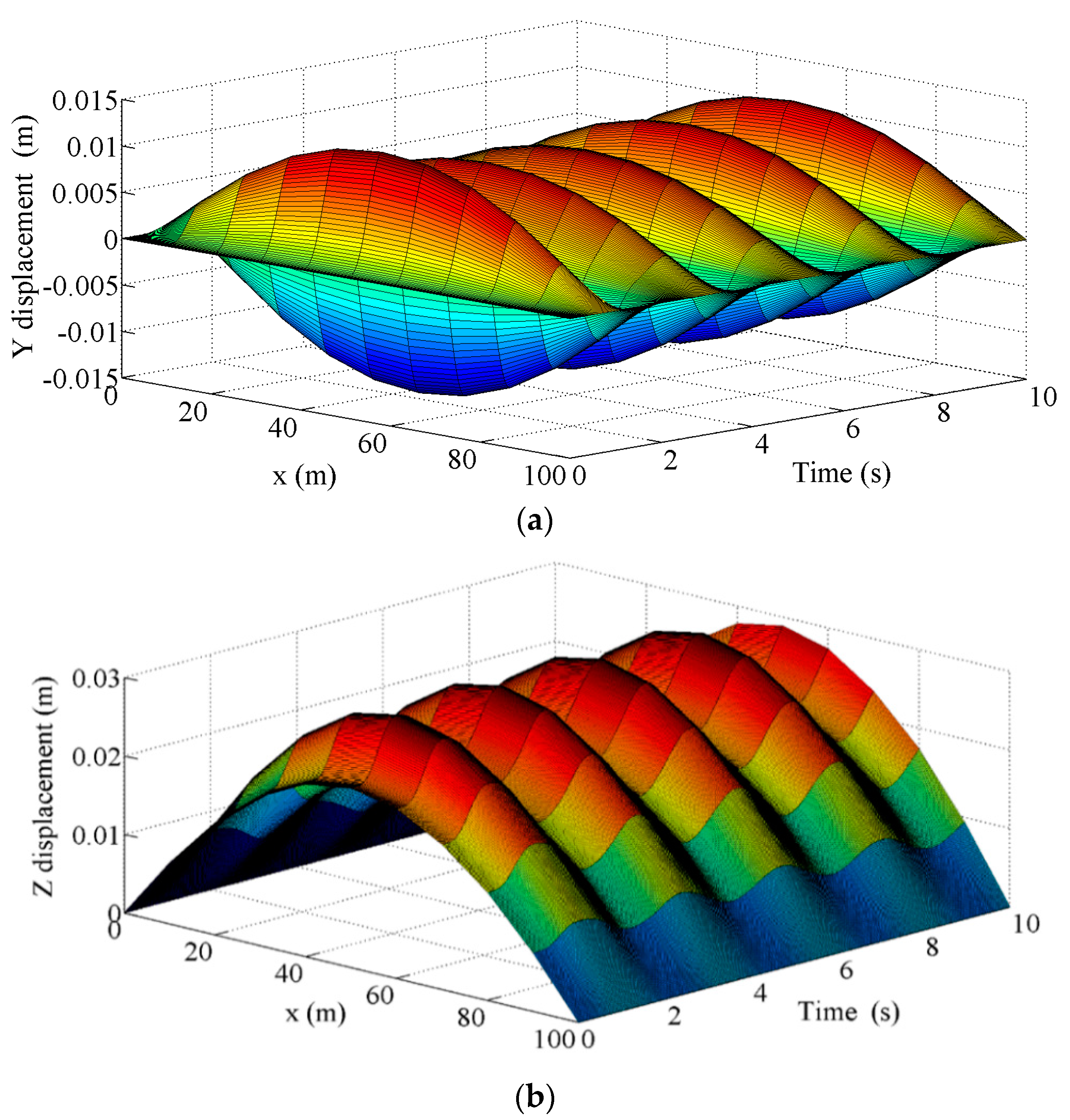
Figure 9.
Hydrodynamic bending moments along the length of the SFT with time: (a) bending moment MY and (b) bending moment MZ.
Figure 9.
Hydrodynamic bending moments along the length of the SFT with time: (a) bending moment MY and (b) bending moment MZ.

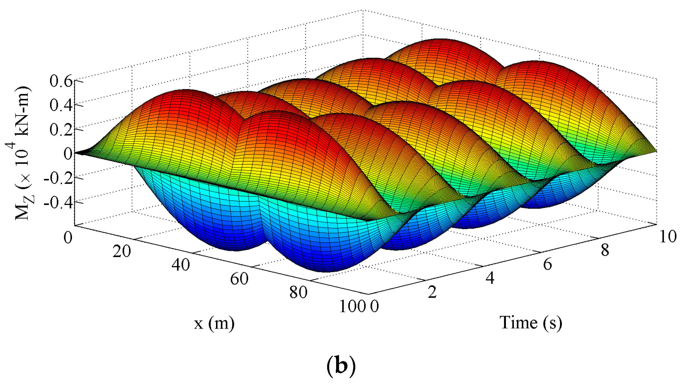
Figure 10.
Ground motion input (El-Centro 1940 site Imperial Valley irrigation district): (a) S00E component; (b) S90W component; and (c) vertical component.
Figure 10.
Ground motion input (El-Centro 1940 site Imperial Valley irrigation district): (a) S00E component; (b) S90W component; and (c) vertical component.

Figure 11.
Comparison of static, hydrodynamic and seismic response envelope curves of the SFT: (a) Y-displacement; (b) bending moment MZ; (c) Z-displacement; and (d) bending moment MY. LC1, Load Combination 1.
Figure 11.
Comparison of static, hydrodynamic and seismic response envelope curves of the SFT: (a) Y-displacement; (b) bending moment MZ; (c) Z-displacement; and (d) bending moment MY. LC1, Load Combination 1.

Figure 12.
SFT dynamic response comparison at mid-span (Section B): (a) Y-displacements; (b) bending moment MZ; (c) Z-displacements; and (d) bending moment MY.
Figure 12.
SFT dynamic response comparison at mid-span (Section B): (a) Y-displacements; (b) bending moment MZ; (c) Z-displacements; and (d) bending moment MY.

Table 1.
Three cable configurations used to support the SFT.
| Mooring configuration | Section A | Section B | Section C |
|---|---|---|---|
| Configuration 1 (C1) |  | | |
| Configuration 2 (C2) | |  | |
| Configuration 3 (C3) | |  | |
Table 2.
Parameters of the SFT tunnel, mooring cables and hydrodynamics.
| Element | Parameter | Unit | Value |
|---|---|---|---|
| Tunnel | Tunnel equivalent density | kg/m3 | 2451 |
| Elastic modulus | N/m2 | 3 × 10¹⁰ | |
| Area | m2 | 5.1 | |
| Moment of inertia | m4 | 12.3 | |
| Length of tunnel | m | 100 | |
| Mooring cables | Elastic modulus | N/m2 | 1.4 × 10¹¹ |
| Diameter of cable | m | 0.06 | |
| Moment of inertia | m4 | 6 × 10⁻⁷ | |
| Cable density | kg/m3 | 7850 | |
| Hydrodynamics | Wave height (H) | m | 1 |
| Time period (T) | s | 2.3 | |
| Surface current velocity () | m/s | 0.1 | |
| Depth of water (h) | m | 30 | |
| Distance of SFT from free surface (h1) | m | 2 | |
| Density of water (ρw) | kg/m3 | 1050 | |
| Drag coefficient (CD) | -- | 1 | |
| Inertia coefficient (CM) | -- | 2 |
Table 3.
Comparison of static displacements and internal forces of the SFT for three mooring configurations at Sections A, B and C.
Table 3.
Comparison of static displacements and internal forces of the SFT for three mooring configurations at Sections A, B and C.
| A | B | C | |||||||
|---|---|---|---|---|---|---|---|---|---|
| C1 | C2 | C3 | C1 | C2 | C3 | C1 | C2 | C3 | |
| (×10−3 rad) | −0.441 | −0.585 | −0.512 | 0.022 | 0.027 | 0.024 | 0.452 | 0.599 | 0.524 |
| (×10−3 rad) | 0.312 | 0.196 | 0.134 | −4 × 10⁻¹³ | −4.9 × 10⁻¹⁴ | −2.2 × 10⁻¹³ | −0.312 | −0.196 | −0.134 |
| (×10−2 m) | 1.395 | 0.918 | 0.663 | 1.716 | 1.114 | 0.791 | 1.395 | 0.918 | 0.663 |
| (×10−2 m) | 2.264 | 2.766 | 2.511 | 2.684 | 3.360 | 3.016 | 2.198 | 2.685 | 2.437 |
| (×103 kN-m) | 10.230 | 11.382 | 10.796 | 10.368 | 17.044 | 13.648 | 8.500 | 9.269 | 8.878 |
| (×103 kN-m) | 7.640 | 5.263 | 3.978 | 9.095 | 5.128 | 2.982 | 7.638 | 5.262 | 3.977 |
| (×102 kN) | 1.459 | 0.659 | 0.231 | −6.2 × 10⁻¹² | −0.800 | −1.228 | −1.459 | −0.659 | −0.230 |
| (×102 kN) | −5.028 | −4.645 | −4.840 | −5.552 | −2.799 | −4.200 | −6.555 | −9.500 | −8.002 |
Table 4.
Modal analysis of the SFT and comparison of the first 20 natural frequencies (Hz) for each cable configuration.
Table 4.
Modal analysis of the SFT and comparison of the first 20 natural frequencies (Hz) for each cable configuration.
| Mode | C1 | C2 | C3 | Mode | C1 | C2 | C3 |
|---|---|---|---|---|---|---|---|
| 1 | 0.5660 | 0.6997 | 0.824 | 11 | 14.0467 | 14.0359 | 14.0408 |
| 2 | 1.2825 | 1.1542 | 1.2144 | 12 | 20.0309 | 20.0309 | 20.0309 |
| 3 | 2.2606 | 2.2606 | 2.2606 | 13 | 20.0417 | 20.0417 | 20.0417 |
| 4 | 2.5041 | 2.5041 | 2.5041 | 14 | 26.2123 | 26.2123 | 26.2123 |
| 5 | 5.0739 | 5.0907 | 5.1103 | 15 | 27.0944 | 27.0975 | 27.1010 |
| 6 | 5.1324 | 5.1025 | 5.1160 | 16 | 27.1051 | 27.0996 | 27.1021 |
| 7 | 8.7454 | 8.7454 | 8.7454 | 17 | 35.1364 | 35.1364 | 35.1364 |
| 8 | 8.9895 | 8.9895 | 8.9895 | 18 | 35.1522 | 35.1522 | 35.1522 |
| 9 | 9.0143 | 9.0143 | 9.0143 | 19 | 43.6074 | 43.6074 | 43.6074 |
| 10 | 13.985 | 13.991 | 13.998 | 20 | 44.1137 | 44.1155 | 44.1176 |
© 2017 by the authors. Licensee MDPI, Basel, Switzerland. This article is an open access article distributed under the terms and conditions of the Creative Commons Attribution (CC BY) license (http://creativecommons.org/licenses/by/4.0/).
Share and Cite
MDPI and ACS Style
Muhammad, N.; Ullah, Z.; Choi, D.-H. Performance Evaluation of Submerged Floating Tunnel Subjected to Hydrodynamic and Seismic Excitations. Appl. Sci. 2017, 7, 1122. https://doi.org/10.3390/app7111122
AMA Style
Muhammad N, Ullah Z, Choi D-H. Performance Evaluation of Submerged Floating Tunnel Subjected to Hydrodynamic and Seismic Excitations. Applied Sciences. 2017; 7(11):1122. https://doi.org/10.3390/app7111122
Chicago/Turabian StyleMuhammad, Naik, Zahid Ullah, and Dong-Ho Choi. 2017. "Performance Evaluation of Submerged Floating Tunnel Subjected to Hydrodynamic and Seismic Excitations" Applied Sciences 7, no. 11: 1122. https://doi.org/10.3390/app7111122
Note that from the first issue of 2016, this journal uses article numbers instead of page numbers. See further details here.