CSO Based Solution for Load Kickback Effect in Deregulated Power Systems


Department of Electrical and Electronics Engineering, SRM University, Chennai 603203, India
*
Author to whom correspondence should be addressed.
Appl. Sci. 2017, 7(11), 1127; https://doi.org/10.3390/app7111127
Submission received: 18 September 2017
/
Accepted: 25 October 2017
/
Published: 1 November 2017
(This article belongs to the Special Issue Distribution Power Systems)
Abstract
:With increase in power demand, load demand values have also risen to a greater extent. Sometimes, these demands are met with the great difficulties. All these difficulties drive us to seek other alternative ways. One such a way demand response (DR) is considered in this paper, it is a new concept that is introduced in the system in order to reduce peak hour stresses. When implementing the demand response, the main setbacks that arise is the load kickback effect, which the sudden rise in demand during non-peak hours that is caused by the overuse of power by consumers, after their constant reduction of power during peak hours. This paper discusses the various kickback load types, and an effective approach to avoid and tackle kickback effect, by an effective method Cat Swarm Optimization (CSO), which is based on studying the movement of cats. The optimization has been implemented on an IEEE 30 bus and 75 bus Indian utility system, and the results are discussed.
1. Introduction
In the previous decades, with the change in the power sector, there has been a tremendous development in load utilization, because of the overwhelming upkeep and types of gear. Now and again, the demand required is high, because of various consumers requesting power in the same time period [1]. Because of this issue, the Generation Companies (GENCO’s) are infrequently not able to meet their client requests, subsequently making them unsatisfied, or to end their agreements. A portion of the developing issues related with power system operation incorporate constrained supply of system assets that thus drives the administrators to operate their systems at their most extreme limit, bringing about consistent price hikes in the power market [2]. All the previously mentioned constraints made us explore and investigate and examine novel ways to build proficient usage of assets in power operations. The author proposed an idea of about power system planning studies, with consideration of Optimal Power Flow (OPF) constraints [3]. On the premise of investigating new ways, demand response (DR) has, as of late, turned into a noteworthy asset in power system operation [4,5].
The utilization of demand response administration in power systems empowers the administrator to productively use their assets, and in addition, enhance the power system’s operation. The utilization of Demand Response Program (DRP) in power system operation builds the benefit of clients and the administrators [6]. Also, consumers who participate in this program are rewarded with incentives for shaving off some of their demand power during peak hours [7,8].
The Federal Energy Regulatory Commission (FERC) report on DR implementation in US utilities and electricity markets in 2006 has classified demand response program in two major categories, namely, Time Based Rate Demand Response Program (TBRDRP), and Incentive Based Demand Response Program (IBDRP) [4]. TBDRP involves changes in price over a day, in accordance with load demand. The higher the demand, the more the price rate, whereas prices decrease in hours where the demand is lower [9]. Here, the consumers are neither penalized nor rewarded, as done in IBDRP. IBDRP involves paying customers a certain amount in the form of incentives, in order for them to shift or curtail their loads during peak hours. Here, the customers are penalized if they fail to curtail the load based on the contract they maintain with the GENCOs. Demand response, when considered theoretically, is satisfying, but when implemented in practical cases, various criteria and constraints need to be checked [10].
Demand response (DR) gives an opportunity in the integration of distributed energy resources as demand side resources (DSR), and encourages them to participate in power system services. The DR program gives support and infrastructure for DSR to produce or consume power with some operating constraints [11]. The main objective of the DR program is balancing the supply and demand power, and maintaining the system without congestion occurring with various demand side resources [12,13]. The proposed work is focused on realizing the unprepared demand response services with real-time control strategies. The main issue associated with implementing demand response in the power systems’ operation network is the load kickback effect [14]. Load kickback effect can be described as the sudden rise in demand during the non-peak hours that is caused by the overuse of power by the consumers after their reduction of power during peak hours [15].
In load kickback effect, the load demand may go beyond the level during the steady state operation before the outage during the system restoration [16]. It is observed that load kickback effect is produced in demand response programs after the load elasticity from DSRs is activated [17]. It may lead to cancellation of the contract, and produce more congestion problems. Controlling the home and commercial loads, like water heater and coolers in peak hours, may reduce the original peak load, but another kickback load is produced, even larger than the original peak load value, after the peak hours [18].This paper discusses the load kickback issue associated with Demand Response while implementing in the power systems. The research outcome provides us with a few solutions to avoid it.
Load kickback effect can be controlled by two methods. The first involves direct load control of electronic devices by the GENCOs. In this method, heavy power consuming devices, like heaters, pumps, and air conditioners, can be directly controlled from the supply station. When the need arises, these devices can be shut directly, to avoid overloading of the system. The second method involves GENCOs with some more incentive rewards to consumers who agree to maintain their loads at a minimum, to avoid overloading of the system after a DR event. The consumers are subsequently rewarded for minimizing their loads.
2. Demand Response Unit Commitment Program
The Traditional Unit Commitment (TUC) is a process of scheduling the power generation, within the system and unit operational limits. Minimizing the generation cost, along with fuel cost and startup cost, is the prime objective of the traditional unit commitment problem [19]. The primary objective of the demand response unit commitment problem is to maximize the profits of the GENCOs using time based demand response program (TBDRP).
PR—is the total profit of the GENCOs and DRSP combined
TRV—is the total revenue calculated from GENCOs and DRSP
TOCOST—is the total operating cost of GENCOs and DRSP combined
Total operating cost varies for GENCOs and consumers:
Total operating cost for GENCOs is represented as
The following section illustrates the various equations associated with demand response unit commitment.
Equality Constraint: The equality constraint gives the power balance between generation and load, (i.e., total generated power should be equal to the demanded power)
Inequality Constraint: The power generation limit should be within the specified generation limits of that unit.
Ramp up Rate: It is the specified limit above which the maximum power generation value cannot be increased for a unit in the next hour.
Ramp down Rate: It is the specified limit below which the minimum power generation value cannot be decreased for a unit in the next hour.
Minimum up time: Once a unit is committed, then for some specific number of hours, it cannot be decommitted.
Minimum down time: Once a unit is decommitted, then for some specific number of hours it cannot be recommitted.
Reserve Constraints: A specified amount of power that is generated by the unit at a particular hour may be used in cases of emergencies, for which it is kept reserved.
Spinning Reserve: The difference between the amount of power generated from all the units synchronized to the system with its present load supplies and losses incurred in the system is called spinning reserve.
Startup Cost of Units: Startup cost can be classified into two different types, namely, hot start cost and cold start cost. Hot start cost is the one where the generator is maintained at minimum temperature, without being shut down. Cold start cost is the one when the generator is shut down, and is started back up once again [20].
3. Cat Swarm Optimization (CSO)
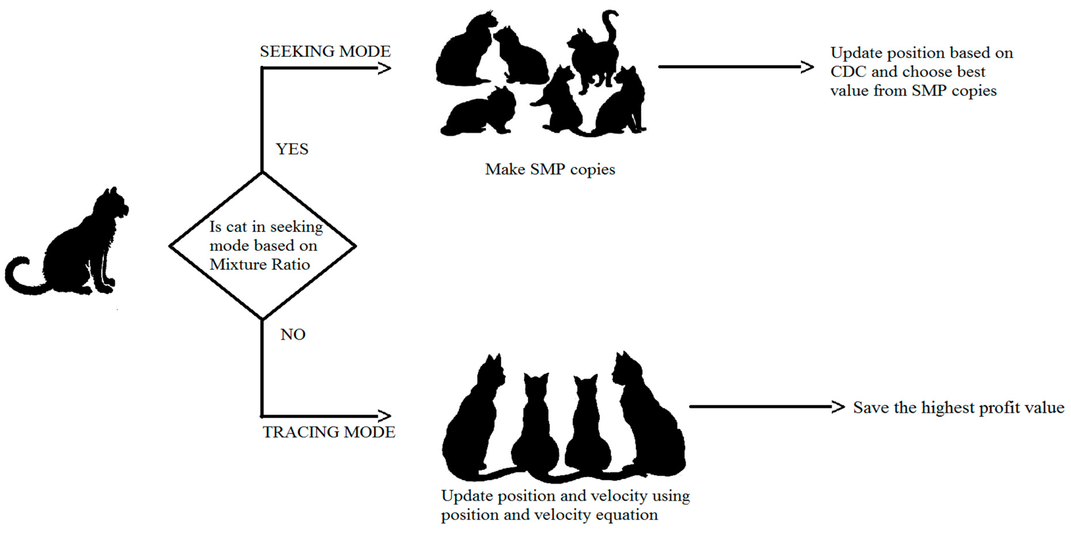
Cat Swarm Optimization is developed by Chu, Tsai, and Pan in 2006, and it can be used to many complex and nonlinear problems [21]. CSO has been successfully applied to a number of power system optimization problems, such as transmission congestion management problems [22], power system stability [23], and reconfiguration problems [24] like optimal placement of Distributed Generator (DG) and Phasor Measurement Unit (PMU) [25]. The constraints impacted by parameters and stagnation issue of Particle Swarm Optimization (PSO) and Differential Evolution (DE) are met by CSO. CSO is a meta-heuristic transformative optimization approach that imitates the characteristic conduct of felines [26]. The main significance of the feline group is that it has a solid interest towards articles that move, and that of the cat group is that it has prevalent chasing aptitudes. Despite the fact that they are dependable and appear to move gradually, they are constantly prepared and attentive towards their environment. On detecting the pray, they chase it rapidly in this manner, spending a lot of vitality [21,27]. These two attributes, that is, the moderate development resting and sudden rapid chasing, are depicted as looking for and following modes. Each of these mode is independently modeled. The pictorial representation of CSO is explained in Figure 1.
3.1. Seeking Mode
There are fouressential factors used in seeking, and these factors are described as [7]
- (a)
- Seeking Memory Pool (SMP): number of cat copies produced.
- (b)
- Seeking Range of selected Dimension (SRD): discrepancy between the new and old in the dimension selected for mutation.
- (c)
- Counts of Dimensions to Change (CDC): number of dimensions to be mutated.
- (d)
- Mixture Ratio (MR): the ratio of the time spent by the cats is resting to observing.
Steps executed in seeking mode:
- (1)
- Randomly choose MR fraction of population seeking cats: rest are declared as tracing cats.
- (2)
- SMP copies of the ith seeking cat are created.
- (3)
- Position of each copy is updated based on CDC, by randomly adding or subtracting SRD fraction.
- (4)
- Error fitness values of copies are evaluated.
- (5)
- Best candidate is picked form all copies and assigned as ith seeking cat.
- (6)
- Repeat step 2 until all seeking cats are involved.
3.2. Tracing Mode
This sub model is modeled when cat is tracing its targets.
In tracing mode, the cats will move in accordance with its own velocity for every dimension. This mode is carried out in 3 steps:
- Velocity of each dimension (Vk,d) is updated according to the following equationwhere d = 1, 2, …, M; xbest,d is position of cat that has best fitness, xk,d is position of cat. c1 is constant and r1 is range.Vk,d = Vk,d + r1 × c1 × (xbest,d − xk,d)
- Check whether the velocities are in possible range of maximum velocity. If the new velocity is over range, it is set equal to the limit.
- Update position of catk according toxk,d = xk,d + vk,d
3.3. Algorithm for Proposed Method
The algorithm for the proposed method solution is discussed below, and the flowchart is explained in Figure 2.
- Step 1: Generate N number of population.
- Step 2: Initialize time t = 0 and i = 0.
- Step 3: Find the overall cost andrevenue for Traditional Unit Commitment (TUC) and Demand Response Service Providers (DRSP)from the data provided, using iterations, and store the values andevaluate the profit for TUC andDRSP using formula Pf = Rv − Tcost.
- Step 4: Check if all units are over andwhether the cat is in seeking mode based on MR value?
- Step 5: If yes, Seeking Mode.Create SMP copies, and update position based on CDC, then take best value from SMP copies.
- Step 6: If no, then Tracing mode.
- Step 7: Update position and velocity by using the equation and , save the highest profit unit.
- Step 8: Check if all cats are updated, if yes, then proceed or else go back to step 4.
- Step 9: Check if maximum iteration is over, if yes, then stop and display the result, else, go back to step 2.
4. Results and Discussion
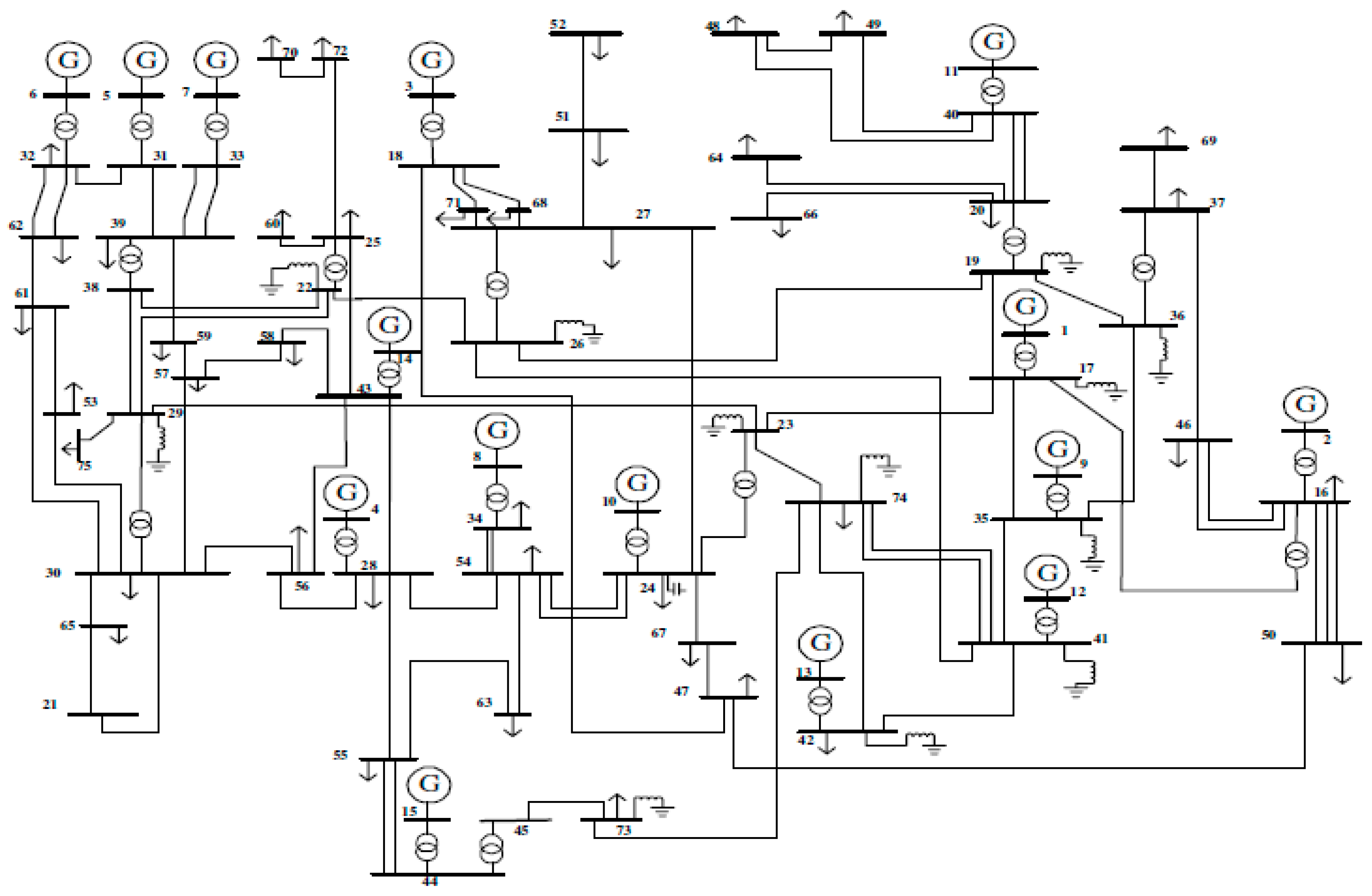
The optimization has been done on two systems, the first being IEEE 30 bus system with 6 generating units, and the second being 75 bus Indian utility system with 15 generating units. The single diagram of the IEEE 30 bus and 75 bus Indian utility systems are given in Figure 3 and Figure 4. The operator data for 30 bus system is given in Table 1 and the fuel and emission cost data is given in Table 2. The operator data for 75 buses Indian utility system is given in Table 3, and the fuel and emission cost data in Table 4.
The optimization algorithm has been implemented on both IEEE 30 bus and 75 bus Indian utility system, and the results have been obtained. The costs of 30 bus system for various cases involving demand response, kickback load, and controlled kickback load are discussed in Table 5. From the table, it can be seen that the profit is high while controlled kickback load is implemented. Same thing has been observed for 75 bus system shown in Table 5, where the various costs have been shown. Here too, it is observed that when controlled kickback load is implemented, there is high rise in profit. Even though the profit is more in a DR regulated environment, it is not taken into consideration, due to the kickback effect.
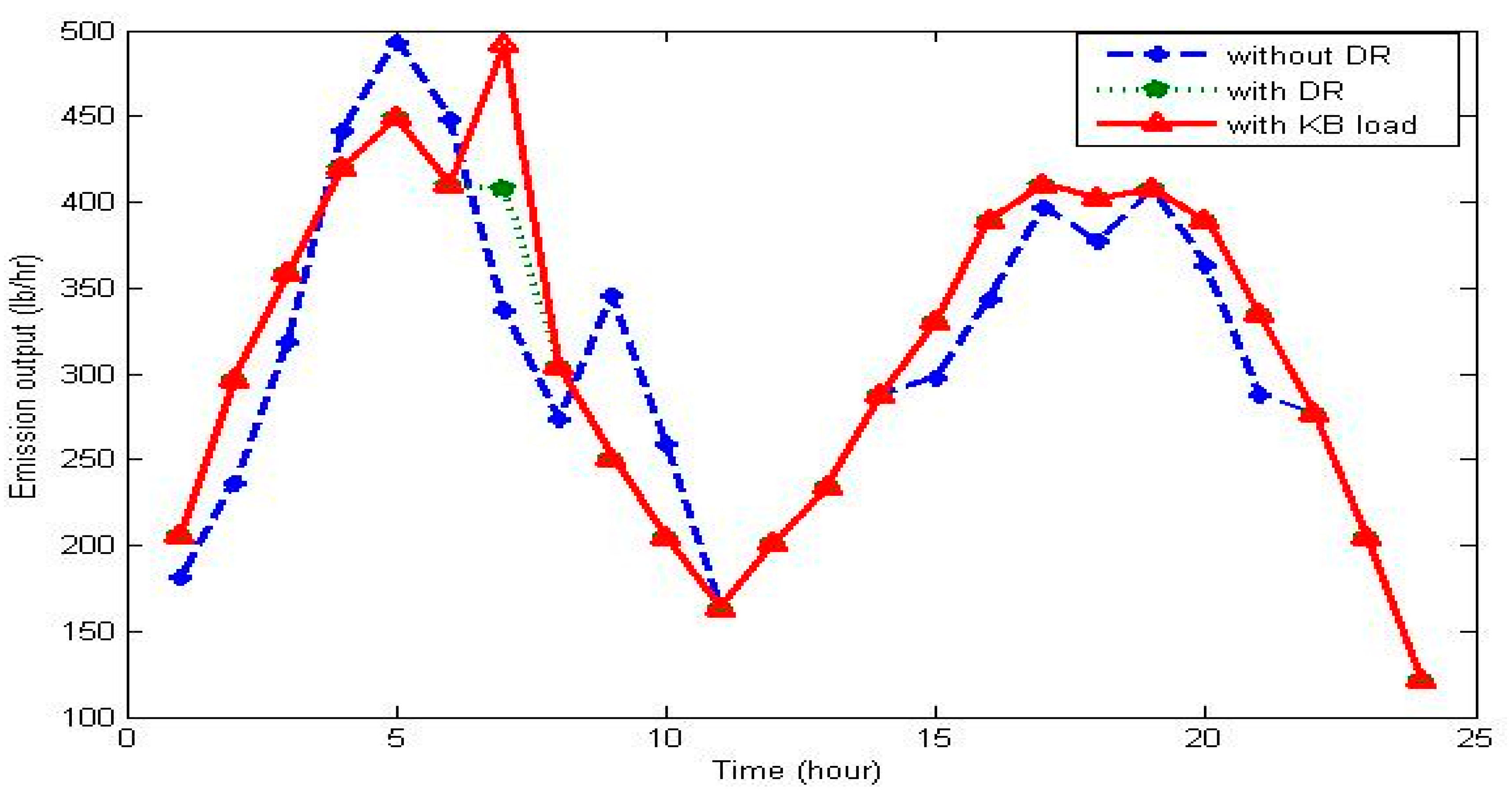
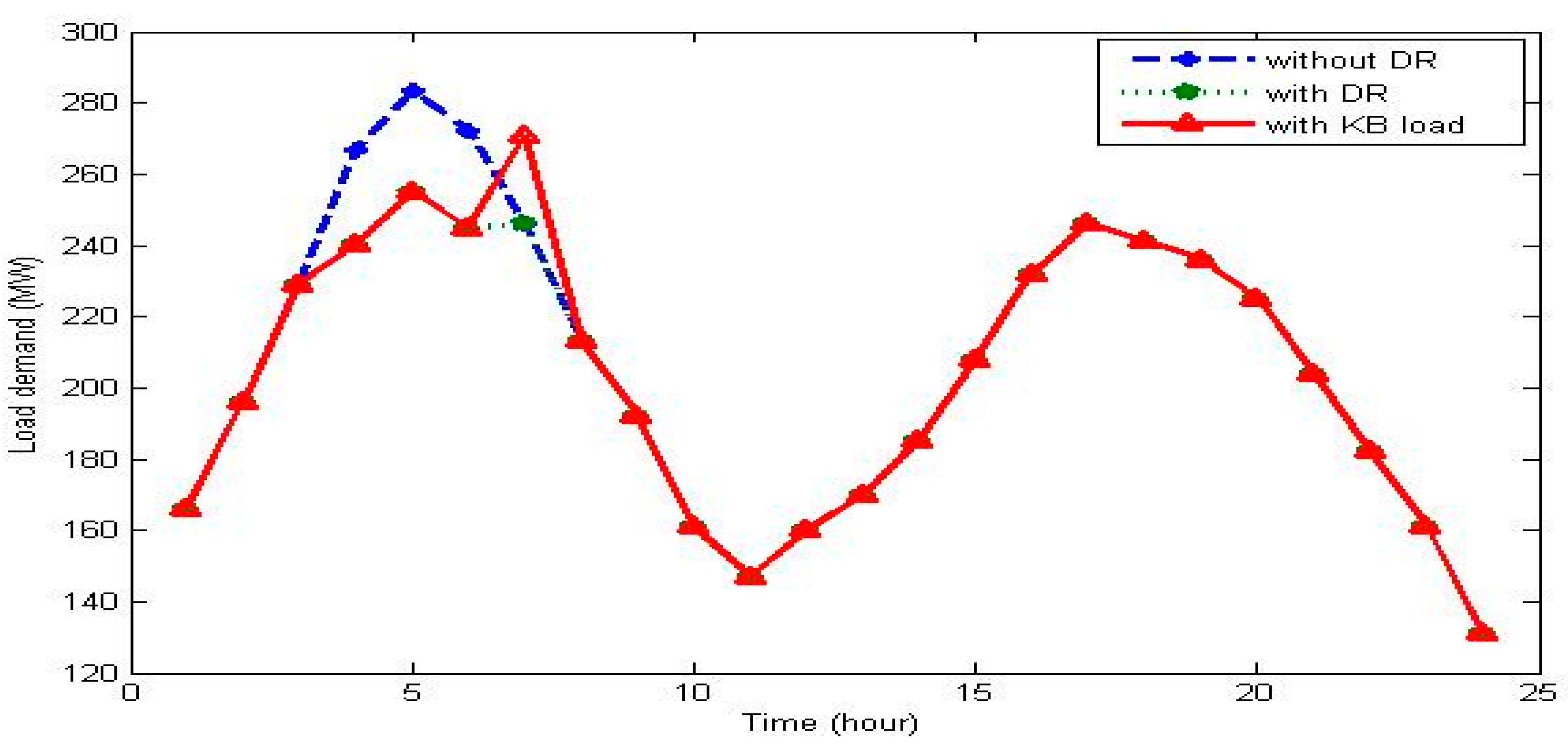
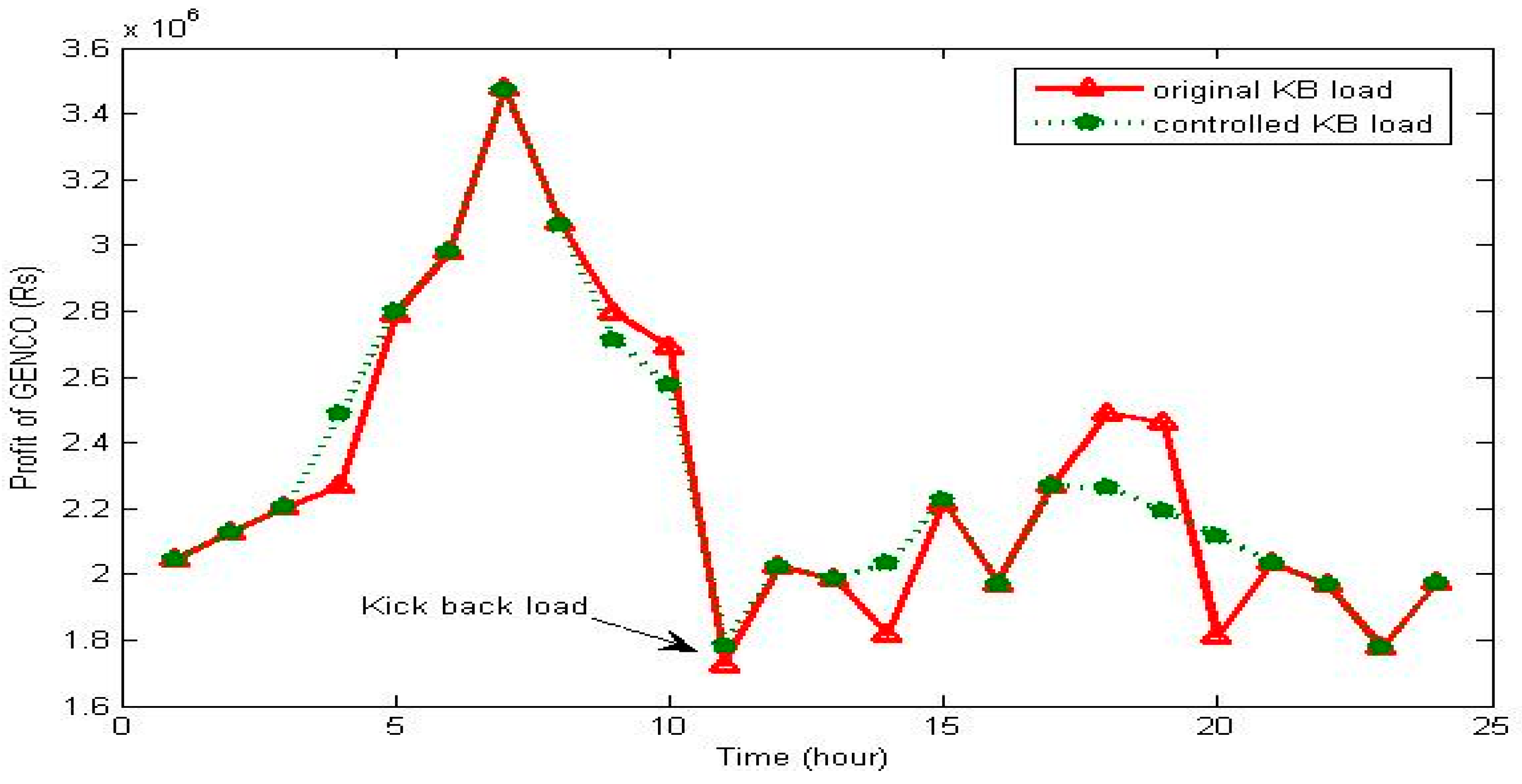
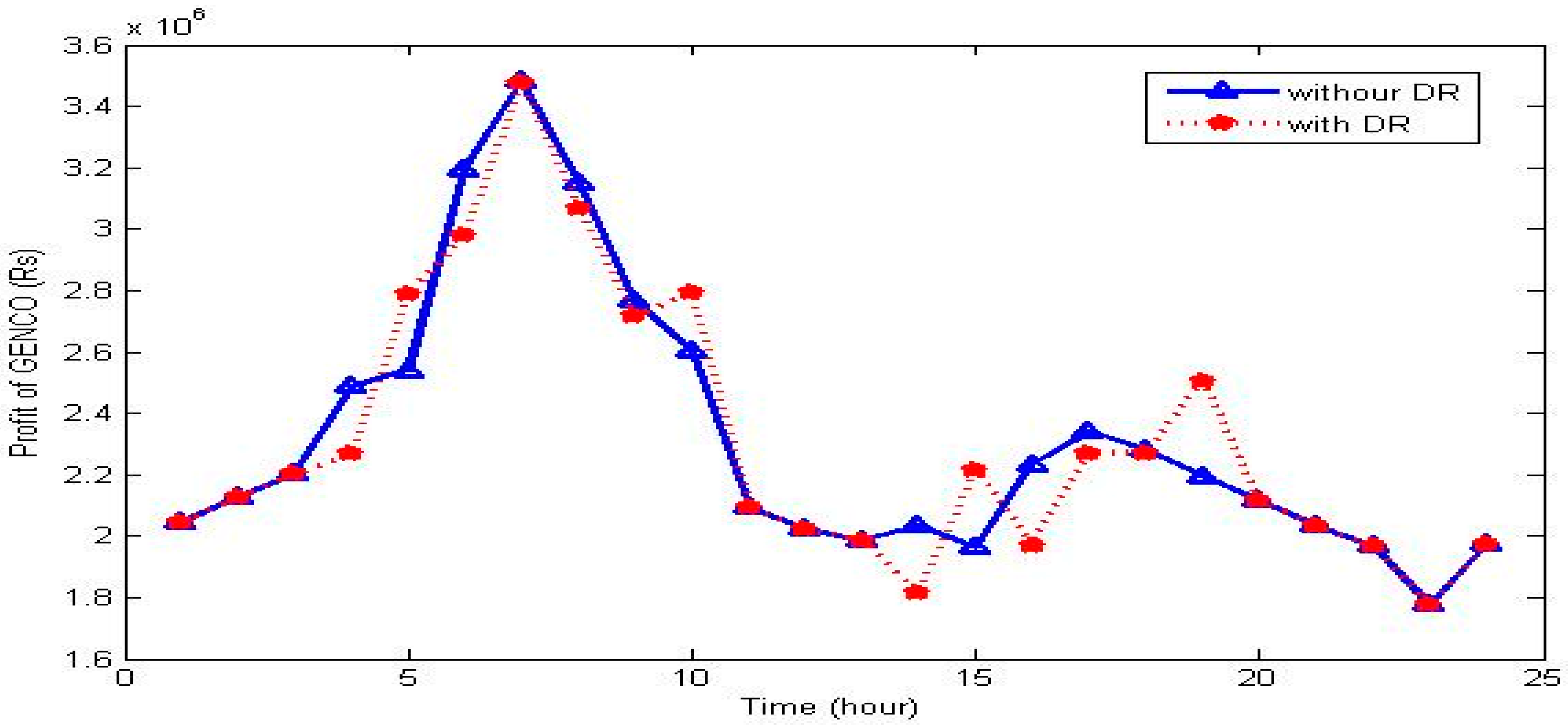
The plots involving various costs and loads have been plotted. Figure 5 shows the plot for emission output versus time for cases involving DR, excluding DR, and with kickback load for 30 bus system. In Figure 5, the emission output for 30 bus system with kickback load hours and off-peak hours, is more compared to without demand response case. However, the total emission output for 30 bus and 75 bus system for 24 h scheduling horizon is less, and is given in Table 6. The emission output has been plotted for 75 bus system in Figure 6. It shows that without demand response case, the emission is more in most of the hours, compared to the other two cases. The load demand versus time with DR, without DR, and with kickback load for 30 bus system has been plotted in Figure 7. The total profit of GENCOs versus time for original kickback load and controlled kickback load for 30 bus system and 75 bus system has been plotted in Figure 8 and Figure 9, respectively.
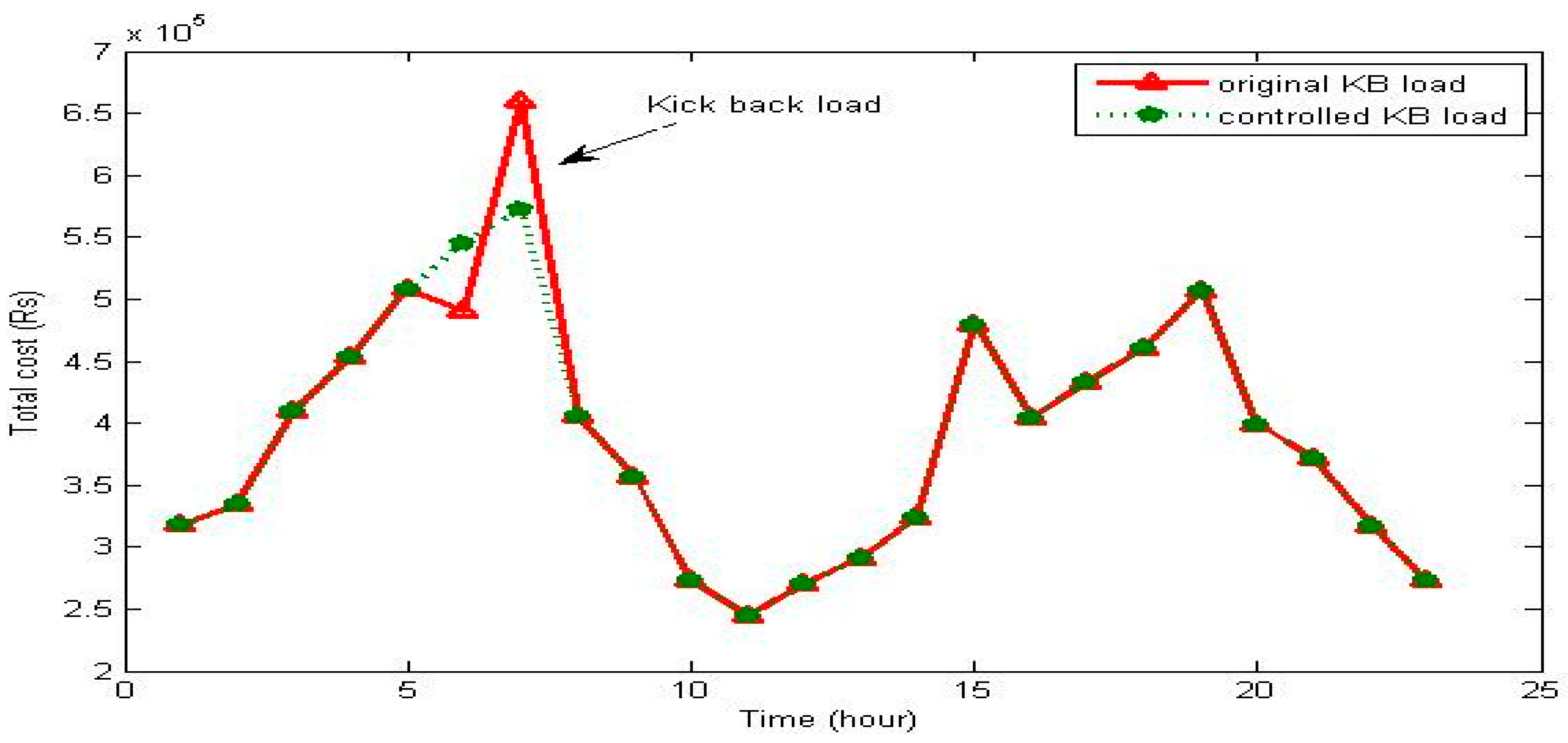
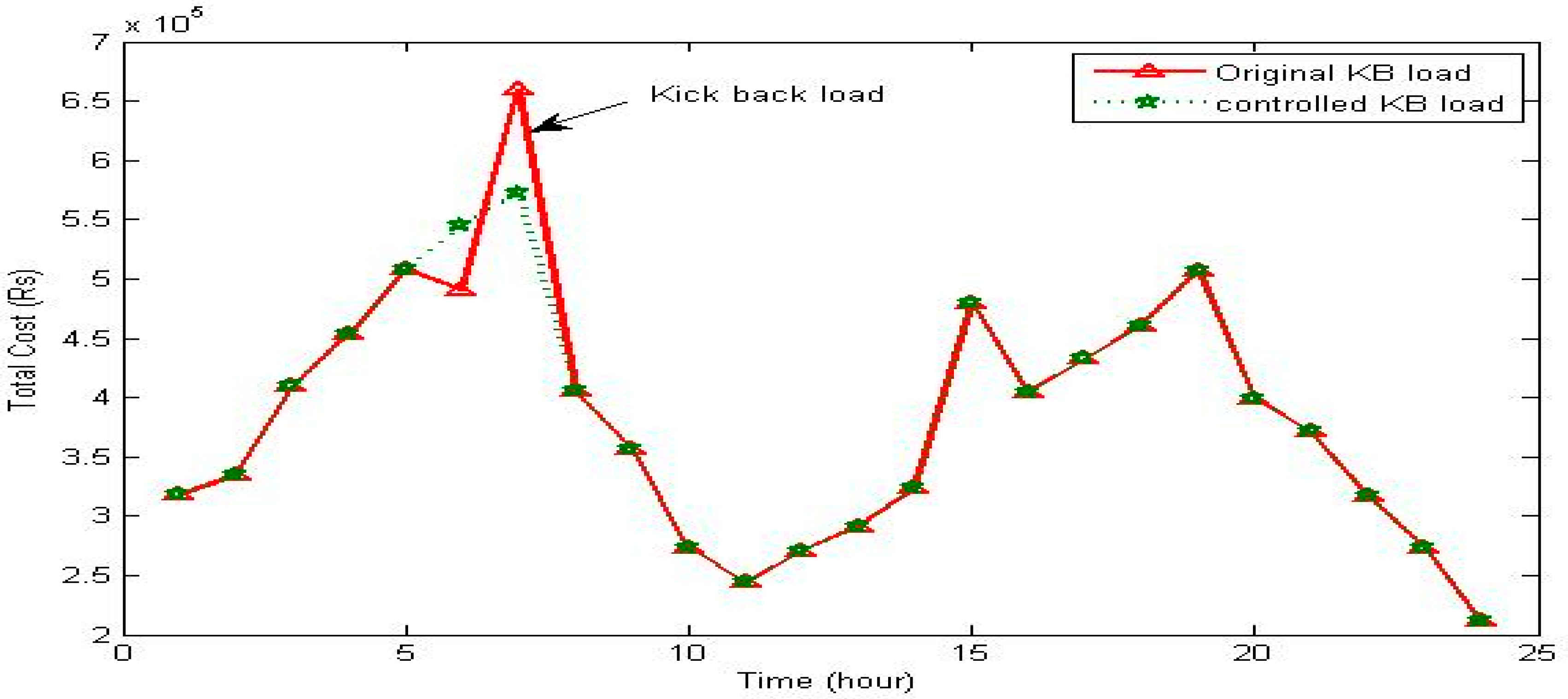
The total cost versus time for original kickback load and controlled kickback load for 30 bus system and 75 bus system has been plotted in Figure 10 and Figure 11. The total generation cost versus time for 30 bus system involving DR and without DR has been shown in Figure 12. The total profit of GENCOs versus time with DR and without DR for 30 bus system and 75 bus system has been shown in Figure 13 and Figure 14. Figure 13 and Figure 14 clearly show the profit is more in most of the hours, except the kickback load-occurring hours in both 30 bus and 75 bus systems.
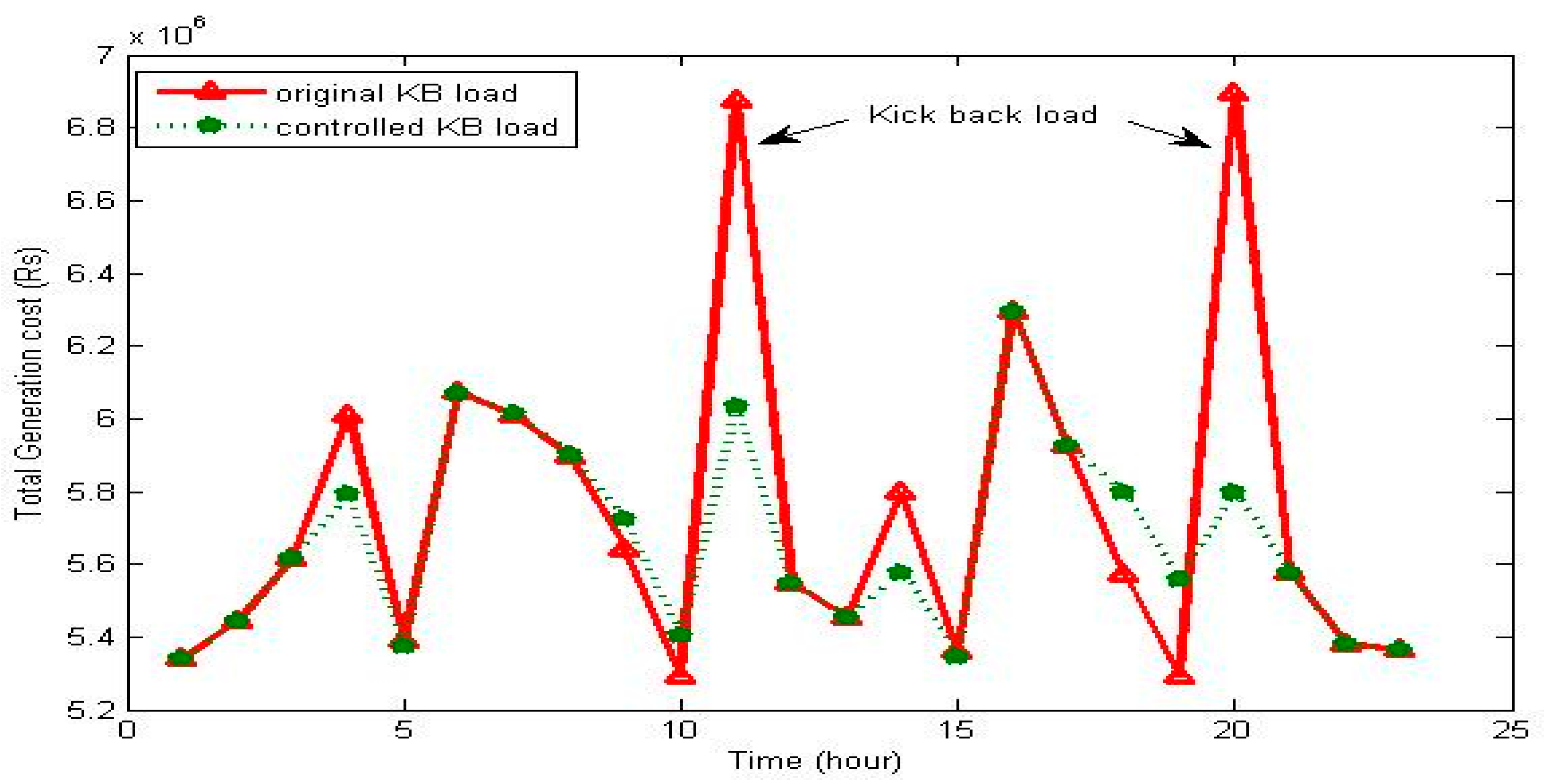
The total generation cost of GENCOs versus time for original kickback load and controlled kickback load for 75 bus systems has been plotted in Figure 15. The original kickback load total generation cost at 11th and 20th hours is comparatively very high, compared to the proposed controlled kickback load case.
5. Conclusions
In this paper, the critical kickback effect aroused when implementing demand response in power systems have been discussed, and the necessary methods to reduce it have been analyzed. Various plots and tables regarding different costs under different scenarios have been discussed. The methodology has been implemented on two systems, IEEE 30 bus system and 75 bus Indian utility systems. Both systems have been tested with critical load kickback effect, and their costs have been optimized using CSO algorithm. It has been observed that the cost in controlled kickback effect is less than the original kickback effect. Consequently; the implemented system has built proficiency on proficient usage of assets in power operations.
Author Contributions
K. Selvakumar and K. Vijayakumar are formulated the problem and obtained the solution. K. Selvakumar and C. S. Boopathi analyzed the results with other methods and wrote the paper.
Conflicts of Interest
The authors declare no conflict of interest.
Nomenclature
| ai, bi, ci | supply curve coefficients of IEEE 10 generating units |
| ramp up rate of unit i | |
| ramp down rate of unit i | |
| minimum up time limit of unit i | |
| minimum down time limit of unit i | |
| hot start cost of unit i | |
| cold start cost of unit i | |
| cold start hour of unit i | |
| PR | total profit of the GENCOs and DRSP combined |
| TRV | total revenue calculated from GENCOs and DRSP |
| TOcost | total operating cost of GENCOs and DRSP combined |
| total operating cost of GENCOs | |
| total operating cost of DRSP | |
| fuel cost of generator unit | |
| power generator output of ith unit at tth hour | |
| total power demand at hour t | |
| minimum generation output power of ith unit | |
| minimum generation output power of ith unit at tth hour | |
| maximum generation output power of ith unit | |
| maximum generation output power of ith unit at tth hour | |
| power generated in the previous hour | |
| unit status of ith unit at tth hour | |
| ONi | number of hours the unit was committed |
| OFFi | number of hours the unit was not committed |
| reserve generation of unit i at tth hour | |
| spinning reserve of unit i | |
| forecasted spot price of unit i | |
| startup cost of unit i |
References
- Paterakis, N.G.; Erdinç, O.; Catalão, J.P. An overview of demand response: Key-elements and international experience. Renew. Sustain. Energy Rev. 2017, 69, 871–891. [Google Scholar] [CrossRef]
- News Releases: January–March 2011. Available online: https://www.ferc.gov/media/news-releases/2011/2011-1.asp (accessed on 15 March 2017).
- Elsaiah, S.; Cai, N.; Benidris, M.; Mitra, J. Fast economic power dispatch method for power system planning studies. IET Gener. Transm. Distrib. 2015, 9, 417–426. [Google Scholar] [CrossRef]
- Qdr, Q. Benefits of Demand Response in Electricity Markets and Recommendations for Achieving Them: A Report to the United States Congress Pursuant to Section 1253 of the Energy Policy Act of 2005; U.S. Department of Energy: Washington, DC, USA, 2005.
- Siano, P. Demand response and smart grids—A survey. Renew. Sustain. Energy Rev. 2014, 30, 461–478. [Google Scholar] [CrossRef]
- Koch, S. Demand Response Methods for Ancillary Services and Renewable Energy Integration in Electric Power Systems. Ph.D. Thesis, Power Systems Laboratory, ETH Zurich, Switzerland, 2012. [Google Scholar]
- International Energy Agency. The Power to Choose—Enhancing Demand Response in Liberalised Electricity Markets; Findings of IEA Demand Response Project; OECD: Paris, France, 2003. [Google Scholar]
- Zhou, S.; Shu, Z.; Gao, Y.; Gooi, H.B.; Chen, S.; Tan, K. Demand response program in Singapore’s wholesale electricity market. Electr. Power Syst. Res. 2017, 142, 279–289. [Google Scholar] [CrossRef]
- Selvakumar, K.; Vijayakumar, K.; Boopathi, C.S. Demand response unit commitment problem solution for maximizing generating companies’ profit. Energies 2017, 10, 1465. [Google Scholar] [CrossRef]
- Gonzalez-Cabrera, N.; Gutierrez-Alcaraz, G. Nodal user’s demand response based on incentive based programs. J. Mod. Power Syst. Clean Energy 2017, 5, 79–90. [Google Scholar] [CrossRef]
- Van Horn, K.; Gross, G. Demand response resources are not all they’re made out to be: The payback effects severely reduce the reported DRR economic and emission benefits. Electr. J. 2013, 26, 86–97. [Google Scholar] [CrossRef]
- Patteeuw, D.; Bruninx, K.; Arteconi, A.; Delarue, E.; D’haeseleer, W.; Helsen, L. Integrated modeling of active demand response with electric heating systems coupled to thermal energy storage systems. Appl. Energy 2015, 151, 306–319. [Google Scholar] [CrossRef] [Green Version]
- Callaway, D.S.; Hiskens, I.A. Achieving controllability of electric loads. Proc. IEEE 2011, 99, 184–199. [Google Scholar] [CrossRef]
- Han, X.; Sossan, F.; Bindner, H.W.; You, S.; Hansen, H.; Cajar, P.D. Load kick-back effects due to activation of demand response in view of distribution grid operation. In Proceedings of the 5th IEEE PES Innovative Smart Grid Technologies, Istanbul, Turkey, 12–15 October 2014. [Google Scholar]
- Han, X.; You, S.; Bindner, H. Critical kick-back mitigation through improved design of demand response. Appl. Therm. Eng. 2017, 114, 1507–1514. [Google Scholar] [CrossRef]
- Lee, S.H.; Wilkins, C.L. A practical approach to appliance load control analysis: A water heater case study. IEEE Trans. Power Syst. 1983, 3, 1007–1013. [Google Scholar] [CrossRef]
- Ericson, T. Direct load control of residential water heaters. Energy Policy 2009, 37, 3502–3512. [Google Scholar] [CrossRef]
- Sehar, F.; Pipattanasomporn, M.; Rahman, S. A peak-load reduction computing tool sensitive to commercial building environmental preferences. Appl. Energy 2016, 161, 279–289. [Google Scholar] [CrossRef]
- Magnago, F.H.; Alemany, J.; Lin, J. Impact of demand response resources on unit commitment and dispatch in a day-ahead electricity market. Electr. Power Energy Syst. 2015, 68, 142–149. [Google Scholar] [CrossRef]
- Morales-España, G.; Ramírez-Elizondo, L.; Hobbs, B.F. Hidden power system inflexibilities imposed by traditional unit commitment formulations. Appl. Energy 2017, 191, 223–238. [Google Scholar] [CrossRef]
- Chu, S.C.; Tsai, P.W.; Pan, J.S. Cat Swarm Optimization. In PRICAI 2006: Trends in Artificial Intelligence; Springer: Berlin, Germany, 2006; pp. 854–858. [Google Scholar]
- Naresh, G.; Raju, M.R.; Narasimham, S.V.L. Coordinated design of power system stabilizers and TCSC using cat swarm optimization algorithm. Swarm Evol. Comput. 2015, 27, 169–179. [Google Scholar] [CrossRef]
- Naresh, G.; Raju, M.R.; Narasimham, S.V.L. Enhancement of Power System Stability Employing Cat Swarm Optimization based PSS. In Proceedings of the IEEE International Conference on Electrical, Electronics, Signals, Communication & Optimization, Visakhapatnam, India, 24–25 January 2015; IEEE: Piscataway, NJ, USA, 2015; pp. 1–7. [Google Scholar]
- Meziane, R.; Boufala, S.; Amara, M.; Hamzi, A. Cat Swarm Algorithm Constructive Method for Hybrid Solar Gas Power System Reconfiguration. In Proceedings of the Renewable and Sustainable Energy Conference (IRSEC), Marrakech, Morocco, 10–13 December 2016; pp. 1–7. [Google Scholar]
- Srivastava, A.; Maheswarapu, S. Optimal PMU Placement for Complete Power System Observability using Binary Cat Swarm Optimization. In Proceedings of the Energy Economics and Environment (ICEEE), Noida, India, 27–28 March 2015; pp. 1–6. [Google Scholar]
- Saha, S.K.; Ghoshal, S.P.; Kar, R.; Mandal, D. Cat swarm optimization algorithm for optimal linear phase FIR filter design. ISA Trans. 2013, 52, 781–794. [Google Scholar] [CrossRef] [PubMed]
- Panda, G.; Pradhan, P.M.; Majhi, B. IIR System Identification using cat swarm optimization. Expert Syst. Appl. 2011, 38, 12671–12683. [Google Scholar] [CrossRef]
Figure 1.
Pictorial representation of Cat Swarm Optimization (CSO) algorithm. SMP, Seeking Memory Pool; CDC, Counts of Dimensions to Change.
Figure 1.
Pictorial representation of Cat Swarm Optimization (CSO) algorithm. SMP, Seeking Memory Pool; CDC, Counts of Dimensions to Change.

Figure 2.
Proposed method flow chart.
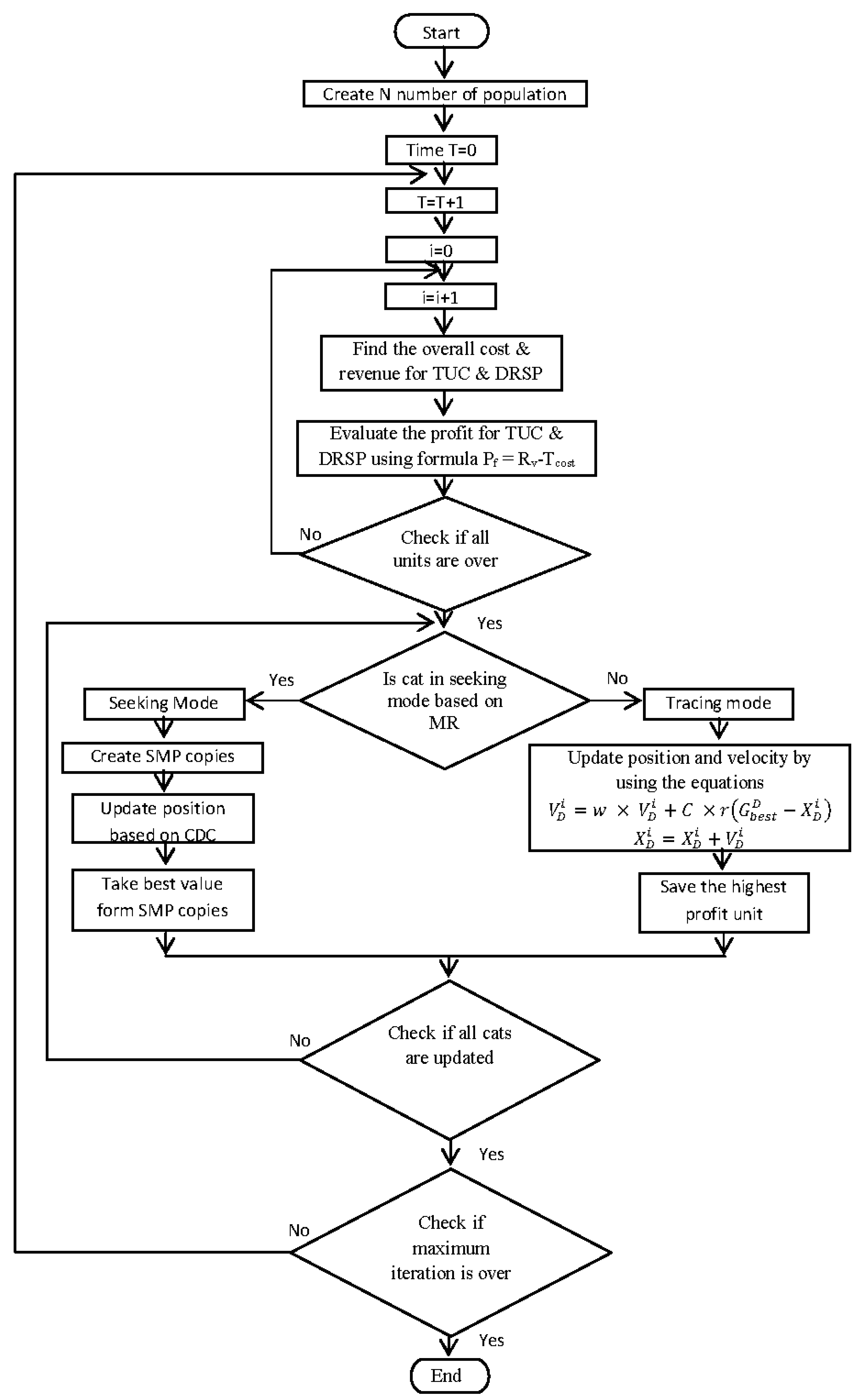
Figure 3.
Single line diagram of IEEE 30 bus test system.
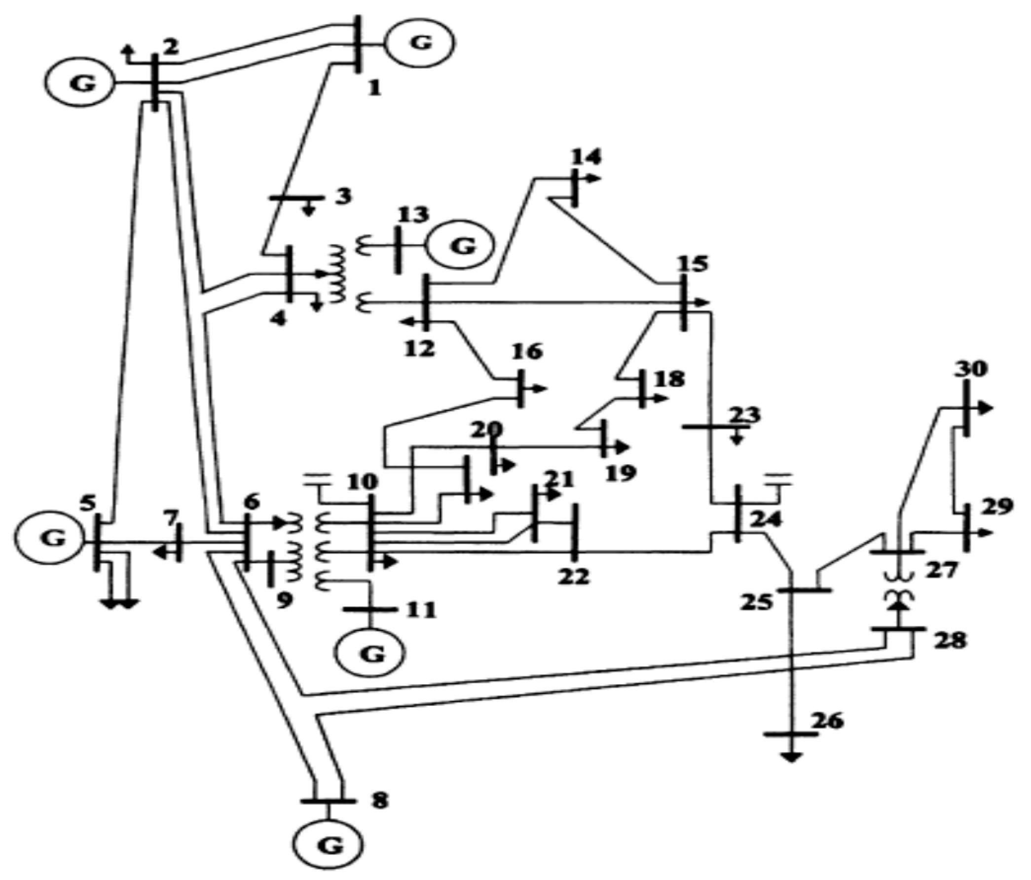
Figure 4.
Single line diagram of 75 bus Indian test system.

Figure 5.
Emission output versus time for without, with demand response (DR) and with Kickback (KB) load for 30 bus system.
Figure 5.
Emission output versus time for without, with demand response (DR) and with Kickback (KB) load for 30 bus system.

Figure 6.
Emission output versus time for without, with DR and with KB load for 75 bus system.
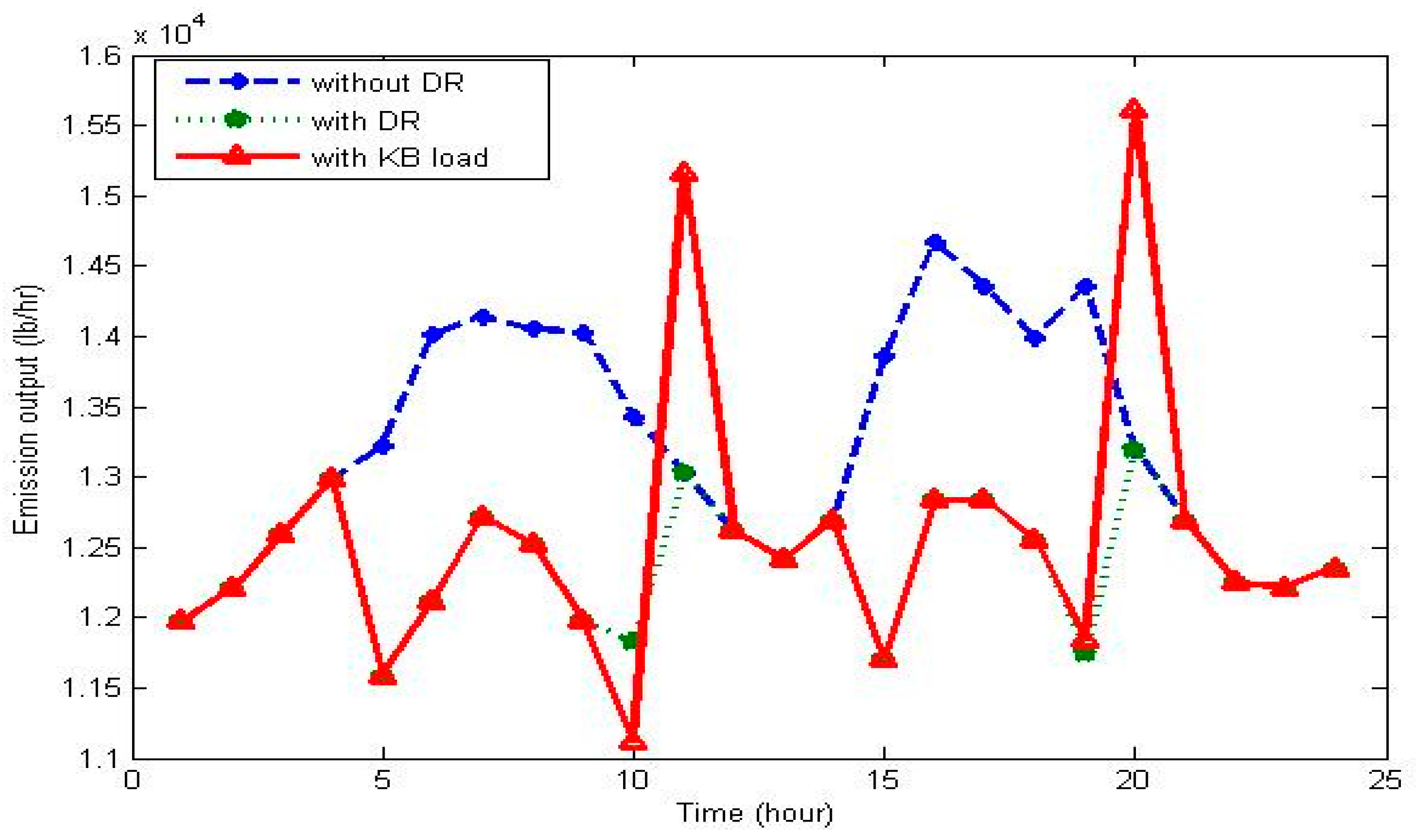
Figure 7.
Load demand versus time without, with DR and with KB load for 30 bus system.

Figure 8.
Total profit of GENCOs versus time for original Kickback load and controlled Kickback load for 30 bus system.
Figure 8.
Total profit of GENCOs versus time for original Kickback load and controlled Kickback load for 30 bus system.
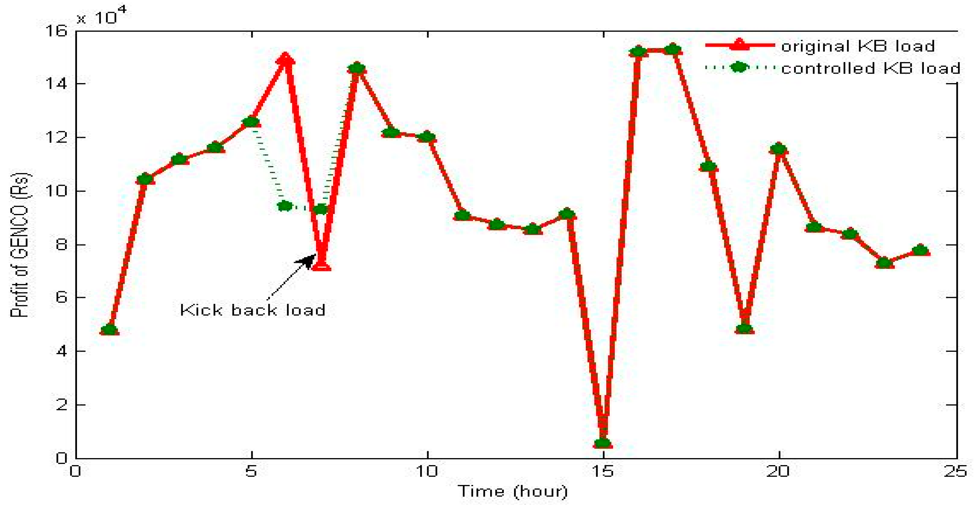
Figure 9.
Total profit of GENCOs versus time for Original KB load and controlled KB load for 75 bus system.
Figure 9.
Total profit of GENCOs versus time for Original KB load and controlled KB load for 75 bus system.

Figure 10.
Total cost versus time for original KB load and controlled KB load for 30 bus system.

Figure 11.
Total cost versus time for original KB load and controlled KB load for 75 bus system.

Figure 12.
Total generation cost versus time for without DR and with DR for 30 bus system.
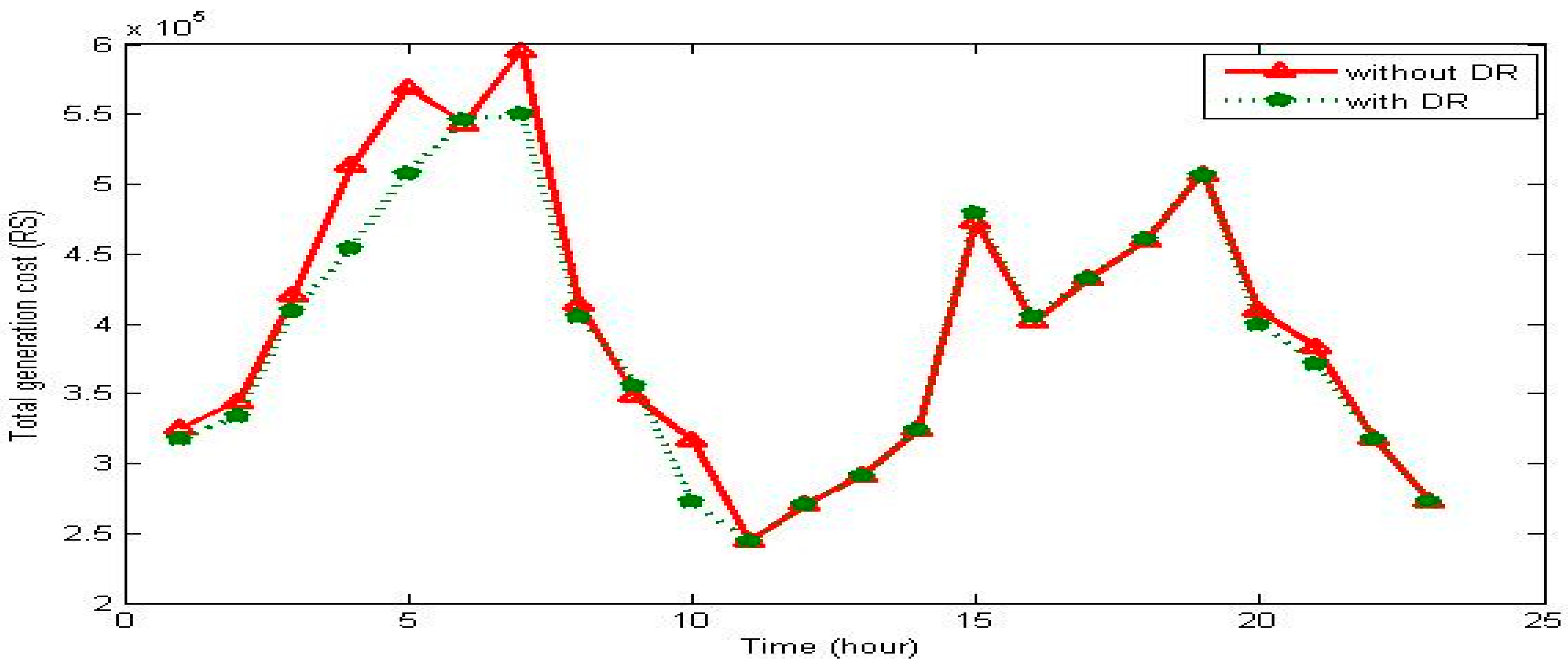
Figure 13.
Total profit of Generation Company versus time for without DR and with DR for 30 bus system.
Figure 13.
Total profit of Generation Company versus time for without DR and with DR for 30 bus system.
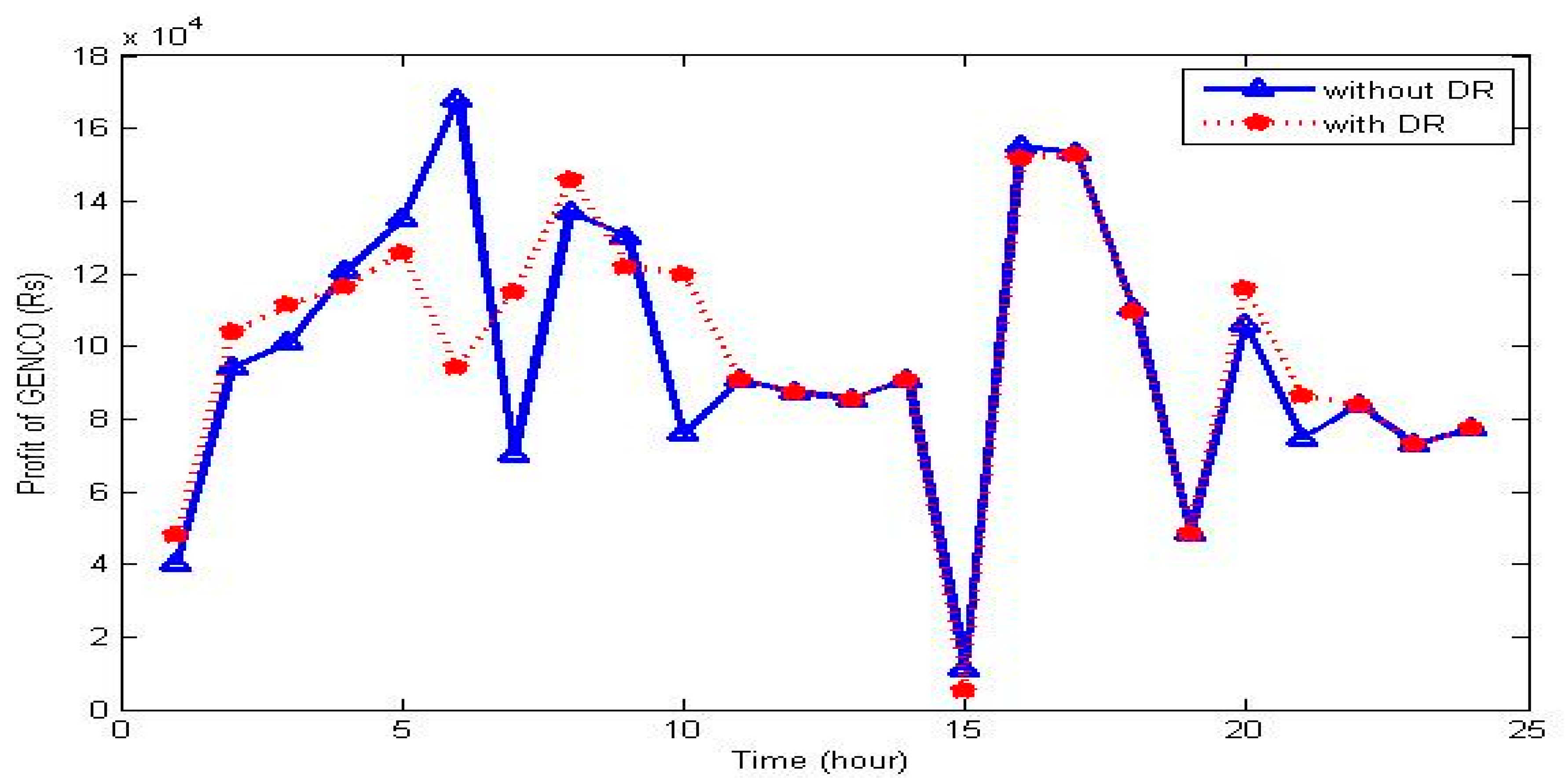
Figure 14.
Total profit of Generation Company versus time for without DR and with DR for 75 bus system.
Figure 14.
Total profit of Generation Company versus time for without DR and with DR for 75 bus system.

Figure 15.
Total generation cost of Generation Company versus time for original KB load and controlled KB load for 75 bus systems.
Figure 15.
Total generation cost of Generation Company versus time for original KB load and controlled KB load for 75 bus systems.

Table 1.
Operator Data for IEEE 30 Bus System.
| Unit No. | Max (MW) | Min (MW) | Ramp Level (MW) | Min up Time (Hr) | Max up Time (Hr) | Shut down Cost ($) | Cold Start (Hr) | Initial Status (Hr) | Hot Start Cost ($) | Cold Start Cost ($) |
|---|---|---|---|---|---|---|---|---|---|---|
| 1 | 200 | 50 | 50 | 1 | 1 | 50 | 2 | −1 | 70 | 176 |
| 2 | 80 | 20 | 20 | 2 | 2 | 60 | 1 | −3 | 74 | 187 |
| 3 | 50 | 15 | 13 | 1 | 1 | 30 | 1 | 2 | 50 | 113 |
| 4 | 35 | 10 | 9 | 1 | 2 | 85 | 1 | 3 | 110 | 267 |
| 5 | 30 | 10 | 8 | 2 | 1 | 52 | 1 | −2 | 72 | 180 |
| 6 | 40 | 12 | 10 | 1 | 1 | 30 | 1 | 2 | 40 | 113 |
Table 2.
Fuel and Emission Cost Data for IEEE 30 Bus System.
| Unit No. | αi | βi | γi | ai | bi | ci |
|---|---|---|---|---|---|---|
| 1 | 0.0126 | −0.9 | 22.983 | 2.4375 | 1300 | 0 |
| 2 | 0.02 | −0.1 | 25.313 | 11.375 | 1105 | 0 |
| 3 | 0.027 | −0.01 | 25.505 | 40.625 | 650 | 0 |
| 4 | 0.0291 | −0.005 | 24.9 | 5.421 | 2112.5 | 0 |
| 5 | 0.029 | −0.004 | 24.7 | 16.25 | 1950 | 0 |
| 6 | 0.0271 | −0.0055 | 25.3 | 16.25 | 1950 | 0 |
Table 3.
Operator Data for Indian 75 Bus System.
| Unit No. | Max (MW) | Min (MW) | Ramp Level (MW) | Min up Time (Hr) | Max up Time (Hr) | Shut down Cost ($) | Cold Start (Hr) | Initial Status (Hr) | Hot Start Cost ($) | Cold Start Cost ($) |
|---|---|---|---|---|---|---|---|---|---|---|
| 1 | 1500 | 100 | 300 | 3 | 2 | 50 | 3 | 4 | 70 | 176 |
| 2 | 300 | 100 | 100 | 3 | 1 | 60 | 2 | 5 | 74 | 187 |
| 3 | 200 | 40 | 100 | 3 | 2 | 30 | 3 | 5 | 50 | 113 |
| 4 | 170 | 40 | 110 | 4 | 2 | 85 | 1 | 7 | 110 | 267 |
| 5 | 240 | 2 | 150 | 1 | 1 | 52 | 1 | 5 | 72 | 180 |
| 6 | 120 | 1 | 120 | 0 | 0 | 30 | 1 | 3 | 40 | 113 |
| 7 | 100 | 1 | 50 | 0 | 1 | 50 | 2 | 4 | 70 | 176 |
| 8 | 100 | 20 | 80 | 1 | 1 | 60 | 1 | 5 | 74 | 187 |
| 9 | 570 | 60 | 214 | 4 | 2 | 30 | 3 | 5 | 50 | 113 |
| 10 | 250 | 30 | 140 | 2 | 1 | 85 | 1 | 7 | 110 | 267 |
| 11 | 200 | 40 | 400 | 0 | 0 | 52 | 2 | 5 | 72 | 180 |
| 12 | 1300 | 80 | 260 | 3 | 1 | 30 | 1 | 3 | 40 | 113 |
| 13 | 900 | 50 | 380 | 3 | 2 | 50 | 2 | 10 | 70 | 176 |
| 14 | 150 | 10 | 80 | 2 | 1 | 60 | 1 | 5 | 74 | 187 |
| 15 | 454 | 20 | 160 | 1 | 1 | 30 | 0 | 5 | 50 | 113 |
Table 4.
Fuel and Emission Cost Data for Indian 75 Bus System.
| Unit No. | αi | βi | γi | ai | bi | ci |
|---|---|---|---|---|---|---|
| 1 | 0.0036 | −0.81 | 24.3 | 1 | 1017.5 | 0 |
| 2 | 0.0035 | −0.1 | 27.023 | 1.75 | 1725.5 | 0 |
| 3 | 0.033 | −0.5 | 27.023 | 2 | 1957.75 | 0 |
| 4 | 0.0034 | −0.3 | 22.07 | 2 | 2008.625 | 0 |
| 5 | 0.038 | −0.81 | 24.3 | 2 | 1957.75 | 0 |
| 6 | 0.033 | −0.5 | 27.023 | 2.25 | 2177.75 | 0 |
| 7 | 0.0034 | −0.03 | 29.04 | 2.25 | 2219.375 | 0 |
| 8 | 0.0039 | −0.02 | 29.03 | 2.25 | 2177.75 | 0 |
| 9 | 0.003 | −0.2 | 27.05 | 1.5 | 1474 | 0 |
| 10 | 0.0034 | −0.3 | 22.07 | 2.125 | 2118.375 | 0 |
| 11 | 0.0034 | −0.25 | 23.01 | 2 | 2026 | 0 |
| 12 | 0.0035 | −0.03 | 21.09 | 0.5 | 511.375 | 0 |
| 13 | 0.0038 | −0.41 | 24.3 | 0.875 | 846.25 | 0 |
| 14 | 0.0034 | −0.2 | 23.06 | 1.875 | 1863.75 | 0 |
| 15 | 0.0036 | −0.1 | 29 | 1.25 | 1253.125 | 0 |
Table 5.
Comparison of Best Results Obtained by Different Cases of Indian 30 Bus System 1.
| Various Cases | Fuel Cost (Rs) | Startup & Shut down Cost (Rs) | DRCost (Rs) | Total Cost (Rs) | Revenue (Rs) | Profit (Rs) | % Profit | Emission Output (lb) |
|---|---|---|---|---|---|---|---|---|
| without DR | 8,917,018 | 466,700 | 0 | 9,383,718 | 11,702,755 | 2,319,037 | 0.19816 | 7294.86 |
| with DR | 8,622,076 | 466,700 | 49,344 | 9,138,120 | 11,497,967 | 2,359,847 | 0.20524 | 7457.98 |
| original KB load | 8,676,450 | 466,700 | 49,344 | 9,192,494 | 11,564,486 | 2,371,992 | 0.20511 | 7541.59 |
| controlled KB load | 8,622,076 | 466,700 | 71,484 | 9,160,260 | 11,497,967 | 2,337,707 | 0.20331 | 7457.98 |
1 DR, demand response.
Table 6.
Comparison of Best Results Obtained by Different Cases of Indian 75 Bus System.
| Various Cases | Fuel Cost (Rs) | Startup & Shut down Cost (Rs) | DR Cost (Rs) | Total Cost (Rs) | Revenue (Rs) | Profit (Rs) | % Profit | Emission Output (lb) |
|---|---|---|---|---|---|---|---|---|
| without DR | 144,625,009 | 815,000 | 0 | 145,440,009 | 201,042,381 | 55,602,372 | 0.27657 | 317,337 |
| with DR | 132,121,681 | 750,000 | 2,262,840 | 135,134,521 | 190,827,785 | 55,693,263 | 0.29185 | 297,636 |
| original KB load | 136,708,617 | 750,000 | 2,262,840 | 139,721,457 | 192,400,892 | 52,679,436 | 0.2738 | 301,567 |
| controlled KB load | 132,121,681 | 750,000 | 2,883,390 | 135,755,071 | 190,827,785 | 55,072,713 | 0.2886 | 297,636 |
© 2017 by the authors. Licensee MDPI, Basel, Switzerland. This article is an open access article distributed under the terms and conditions of the Creative Commons Attribution (CC BY) license (http://creativecommons.org/licenses/by/4.0/).
Share and Cite
MDPI and ACS Style
Selvakumar, K.; Vijayakumar, K.; Boopathi, C.S. CSO Based Solution for Load Kickback Effect in Deregulated Power Systems. Appl. Sci. 2017, 7, 1127. https://doi.org/10.3390/app7111127
AMA Style
Selvakumar K, Vijayakumar K, Boopathi CS. CSO Based Solution for Load Kickback Effect in Deregulated Power Systems. Applied Sciences. 2017; 7(11):1127. https://doi.org/10.3390/app7111127
Chicago/Turabian StyleSelvakumar, K., K. Vijayakumar, and C.S. Boopathi. 2017. "CSO Based Solution for Load Kickback Effect in Deregulated Power Systems" Applied Sciences 7, no. 11: 1127. https://doi.org/10.3390/app7111127
Note that from the first issue of 2016, this journal uses article numbers instead of page numbers. See further details here.