A Robust Optimization Strategy for Domestic Electric Water Heater Load Scheduling under Uncertainties


1
Key Laboratory of Smart Grid of Ministry of Education, Tianjin University, Tianjin 300072, China
2
State Grid Chengdu Power Supply Company, Chengdu 610041, China
*
Author to whom correspondence should be addressed.
Appl. Sci. 2017, 7(11), 1136; https://doi.org/10.3390/app7111136
Submission received: 3 October 2017
/
Revised: 31 October 2017
/
Accepted: 1 November 2017
/
Published: 5 November 2017
(This article belongs to the Special Issue Smart Home and Energy Management Systems)
Abstract
:In this paper, a robust optimization strategy is developed to handle the uncertainties for domestic electric water heater load scheduling. At first, the uncertain parameters, including hot water demand and ambient temperature, are described as the intervals, and are further divided into different robust levels in order to control the degree of the conservatism. Based on this, traditional load scheduling problem is rebuilt by bringing the intervals and robust levels into the constraints, and are thus transformed into the equivalent deterministic optimization problem, which can be solved by existing tools. Simulation results demonstrate that the schedules obtained under different robust levels are of complete robustness. Furthermore, in order to offer users the most optimal robust level, the trade-off between the electricity bill and conservatism degree are also discussed.
1. Introduction
With the emergence of smart grids and the increase of electricity demand, home energy management system (HEMS) is attracting increasing attention as an important part of demand side of management. HEMS is able to improve the implementation of the distributed energy resource and shift the demand to off-peak periods [1]. At present, monetary incentives are the major driving force for residential consumers to participate in household load management. Flexible pricing schemes, such as critical peak pricing (CPP), time-of-use (TOU), and real-time pricing (RTP), are designed by utilities to encourage users to actively respond to demand side management [2,3].
Responding to the various pricing schemes, load scheduling plays an essential role in HEMS [4,5], which optimizes working schedules for household appliances to reduce the electricity bill and improves the power consumption efficiency while satisfying the consumers’ comfort constraints [6]. Domestic electric water heaters (DEWH) are considered as well suited for demand side management, because of their high nominal power ratings combined with large thermal buffer capacities [7].
In addition, DEWH load accounts for a considerable share of the whole household load. In USA and Japan, DEWH load contributes as much as 17% and 27% to the total household electrical energy consumption [8,9]. Therefore, the scheduling strategies for DEWH load are vital for HEMS to help consumers to automatically obtain optimal DEWH load schedules. With such background, several valuable works have been done on DEWH load scheduling.
There are rich scheduling algorithms that are aimed to minimize the electricity payment under different rate structures, and various strategies for DEWH scheduling have been studied extensively. In [10], three consumer strategies were studied to schedule DEWHs under dynamic pricing, including timed power interruption, price-sensitive thermostat, and double period setback timer. Furthermore, a series of scenarios with different set points of water temperature in tank (between 120 and 140 °F) were analyzed to study the relevance of electricity cost to set points. In [11], DEWH load was deemed as an example of thermostatically controlled household loads, and scheduled through a linear-sequential-optimization-enhanced, multi-loop algorithm. A transactive control strategy was utilized to schedule the DEWH load iteratively according to the sorted day-ahead forecast price. Though the proposed optimization strategy is indeed simple, the created schedules are not necessarily cost-efficient. Given this deficiency, Reference [12] put forward a traversal-and-pruning (TP) algorithm to address the optimization problem of DEWH load scheduling. To handle the curse of dimensionality of the solution tree, a novel method named “Inferior Pruning” was proposed to traverse to the superior node’s sub-nodes. Simulation results indicated that approximately 20% energy cost was reduced with the same comfort level as that of the reference method.
However, in the above literatures, all of the relevant parameter values in household load scheduling are considered to be forecast completely accurately, which is not the real case in practice. Generally, forecast errors are inevitable for some parameters such as weather conditions, consumer behaviors, etc. [13]. With such a background, studying methods to tackle the uncertain parameters caused by forecast inaccuracy is of great significance for household load scheduling. In [14,15], a two-stage stochastic optimization approach was introduced to tackle the uncertain household load scheduling. The decision variables were separated into two types of sub-variables named here-and-now variables, which are asked for decision-making at a given time and wait-and-see variables that can be determined later when enough information is available. In [16,17], fuzzy programming was introduced to tackle the uncertain optimization in HEMS, in which uncertain parameters, like electricity prices and outdoor temperature, were described by fuzzy parameters.
In comparison to traditional methodologies for uncertain optimization problems, such as stochastic programming and fuzzy programming, interval analysis (a kind of set-theoretical and non-probabilistic method) only requires the bounds of the magnitude of uncertainties, not necessarily requiring the specific probabilistic distribution densities. As less uncertainty knowledge is needed, interval number is suitable for describing the uncertain parameters in DEWH load scheduling with limited uncertainty knowledge. Therefore, in this paper, the uncertain parameters in DEWH are modeled as interval numbers, and the uncertainties are divided into different robust levels. Then, the DEWH load scheduling problem is rebuilt under different robust levels and its constraints are transformed into an equivalent form for solving. Simulation results show that the proposed method can provide consumers with the robust schedules with different robust levels. In addition, the trade-off between the electricity bill and the conservatism level can be made to offer a diversity of options for consumers.
2. The Domestic Electric Water Heaters (DEWH) Load Scheduling Problem
The DEWH load scheduling problem has been summarized into a mathematical programming problem, of which the objective is to minimize the consumers’ electricity bill under flexible tariff structure and the constraints are about device limits and thermal comfort [18,19,20,21]. The scheduling problem is built on the thermal dynamic model of a DEWH, which describes the process of the heating and coasting of water in the tank. Figure 1 shows the water temperature curve in a DEWH tank.
As shown in Figure 1, there are two operation states for a DEWH, being “switch on” state and “standby” state. When the water temperature in tank drops to the lower threshold, then the water heater is switched on to recover the water temperature into comfort zone; when the water temperature in tank reaches the upper threshold, the water heater becomes standby. The thermal dynamic model is used to describe the behavior of a DEWH [11]. When only the standby heat loss is considered, there is
where denotes the temperature of hot water in tank at the time ; denotes the ambient temperature/cold water inlet temperature at the time ; represents the on/off state of DEWH over period (1-on; 0-off ); and, the constants Q, R and C are equivalent thermal parameters, which represent the electric water heater capacity, thermal resistance, and thermal capacitance, respectively.
Moreover, when the hot water demand is considered, Equation (1) is modified as
where is just the calculated in (1), is the water demand at the time , and M is the mass of water in the tank. Combining the two equations, one united expression is given to simplify the thermal model as follows:
Equation (3) calculates the water temperature in tank in each step straightforwardly. It lays the foundation for the DEWH load scheduling. The detail proof process refers to Appendix A.
However, this temperature-driven running mode might be not cost-efficient under the flexible pricing schemes. The time-varying electricity price enable the DEWH load to operate more flexibly and cost-efficiently, motivating the DEWH to preheat the water in tank in the low electricity price periods and reduce the load in the peak-price periods [7].
So, when considering the time-varying prices, the DEWH load scheduling is modeled as follows. The objective function is to minimize the next 24-h total electricity expense and the constraints limit the water temperature under the consumers’ setting zone. The states of the DEWH are the decision variables in the model, which should be solved for consumers as guiding schedules for the following day. Mathematically, the DEWH load scheduling can be formulated as [12]:
subjected to
where N is the number of all the time steps over the scheduling horizon and denotes the rated power of DEWH; represents the time-varying prices in the nth time step.
Hence, the DEWH load scheduling problem can be summarized into a linear optimization problem, the optimal solution of the problem is exactly the DEWH load schedule that the consumers require.
3. DEWH Load Scheduling under Different Robust Levels
3.1. The Bounded Uncertainties of the Hot Water Demand and Ambient Temperature
In the aforementioned scheduling problem, the purpose of the DEWH is to maximize the economic benefits, and meanwhile keep the hot water temperature profiles within the comfort zones. While due to the randomness in the environment and human behaviors, the parameters in the DEWH load scheduling problem, such as the ambient temperature and the hot water demand, which cannot be predicted precisely. The uncertain parameters may lead to the violations on comfort zones and ineffectiveness of the original optimal schedule. Therefore, the impact of diverse levels of uncertain water demand and ambient temperature on hot water temperature in tank should be discussed in detail.
According to the analysis in Reference [16,22], it is reasonable to describe the uncertainties of the hot water demand and ambient temperature with uncertain-but-bounded parameters whose boundaries are always based on predicted values. The two uncertain-but-bounded parameters, water demand and ambient temperature, can be expressed as intervals by introducing two auxiliary parameters. Moreover, to control the degree of conservatism of the uncertain parameters, one pair of robust level indicators are predefined to divide the uncertainties of water demand and ambient temperature into different grades, which indicates the consumers’ optimistic degree for the predicted uncertain-but-bounded parameters in household load scheduling. Given this background, the intervals under different levels of the uncertain water demand in nth time step is described as:
Similarly, the intervals under different levels of the uncertain ambient temperature in nth time step is described as:
where and are the auxiliary parameters for intervals of water demand and ambient temperature respectively, making the uncertain parameters ranged in the intervals. Accordingly, and represent the robust levels for the two uncertain parameters. If the robust levels are equal to 0, it means that consumers are very confident and optimistic about the predicted values. In such situation, the intervals are compressed into real numbers and the uncertain parameters lose the uncertain characteristic, if the robust levels are equal to and , then it means that consumers are completely distrustful and pessimistic about the predicted values. In this case, the range of intervals reaches the maximum. When the robust levels are set between zero and maximum, diverse intervals under different levels of the uncertainties are created.
In view of the analysis in Section 2, Equation (3) is the thermal dynamic model of a DEWH with deterministic parameters. If the uncertainties as shown in Equations (7) and (10) are considered, it is modified as:
Equation (13) is the dynamic temperature model with bounded uncertainties, showing that the water temperature in tank will fluctuate in a certain range under uncertain-but-bounded water demand and ambient temperature. Its uncertain level is influenced by the robust levels and .
3.2. The Scheduling Problem under Different Robust Levels
To improve the flexibility of energy production and consumption, various time-varying pricing mechanisms are implemented around the world. In this paper, RTP price is considered as the time-varying pricing mechanism used in the analysis, as its retail electric prices update frequently to take the variations in the cost of the power supply into account [23].
When considering the uncertainties, the optimization problem of DEWH load scheduling is still to minimize the electricity bill but subjects to comfort constraints with different robust levels. Therefore, the scheduling problem can be rebuilt as follow:
As the hot water temperature in tank in each step is involved with the uncertain auxiliary parameters and , the optimization problem formulated by (14–16), obviously, could not be solved directly. To address this uncertain optimization problem, it is necessary to obtain the bounds of uncertain hot water temperature in tank. Hence, there is
The hot water temperature fluctuates in its interval, while the auxiliary parameters change. In order to figure out the constraints with uncertainties, the boundaries of the interval should be calculated. Appendix B fortunately indicates that
With such background, the constraint (15) could be transformed into
Besides, to make this optimization problem solvable, Equation (19), which is an uncertain inequality constraint, is transformed into two deterministic constraints, which is given by
Based on the above analysis, the optimization problem of DEWH load scheduling with different robust levels could be formulated as integer linear programming, of which the objective function is shown in Equation (4) and the constraints are the Equations (7)–(13), (16) and (20).
So far, the optimization problem has been transformed to an integer linear programming problem, and many existing methods, tools, and commercial software are available to obtain the optimal solution. Among the abundant methods, the heuristic-based evolutionary algorithm like particle swarm optimization (PSO) [21], model predictive method [24], and commercial software CPLEX (Version 12.6.3.0, IBM, New York, USA, 2016) [25] and MOSEK(Version 7.1.0.63, ApS, Copenhagen, Denmark, 2016) [26] are some of the representative ones. Especially, IBM ILOG CPLEX® Optimizer is used in this paper to solve the problem considering its strong capability.
4. Simulation Results
In this paper, a day-ahead DEWH load scheduling (from 0 a.m. to 12 p.m.) is considered. The length of each time step, Δt, is set as 15 min. Chosen from the 2012 American Society of Heating, Refrigerating, and Air-Conditioning Engineers (ASHRAE,) Hand-book [27], the specific parameters in the thermal dynamic model of DEWH are listed in Table 1. The daily real-time prices are assumed to be known. The RTP values refer to [16], as shown in Figure 2.
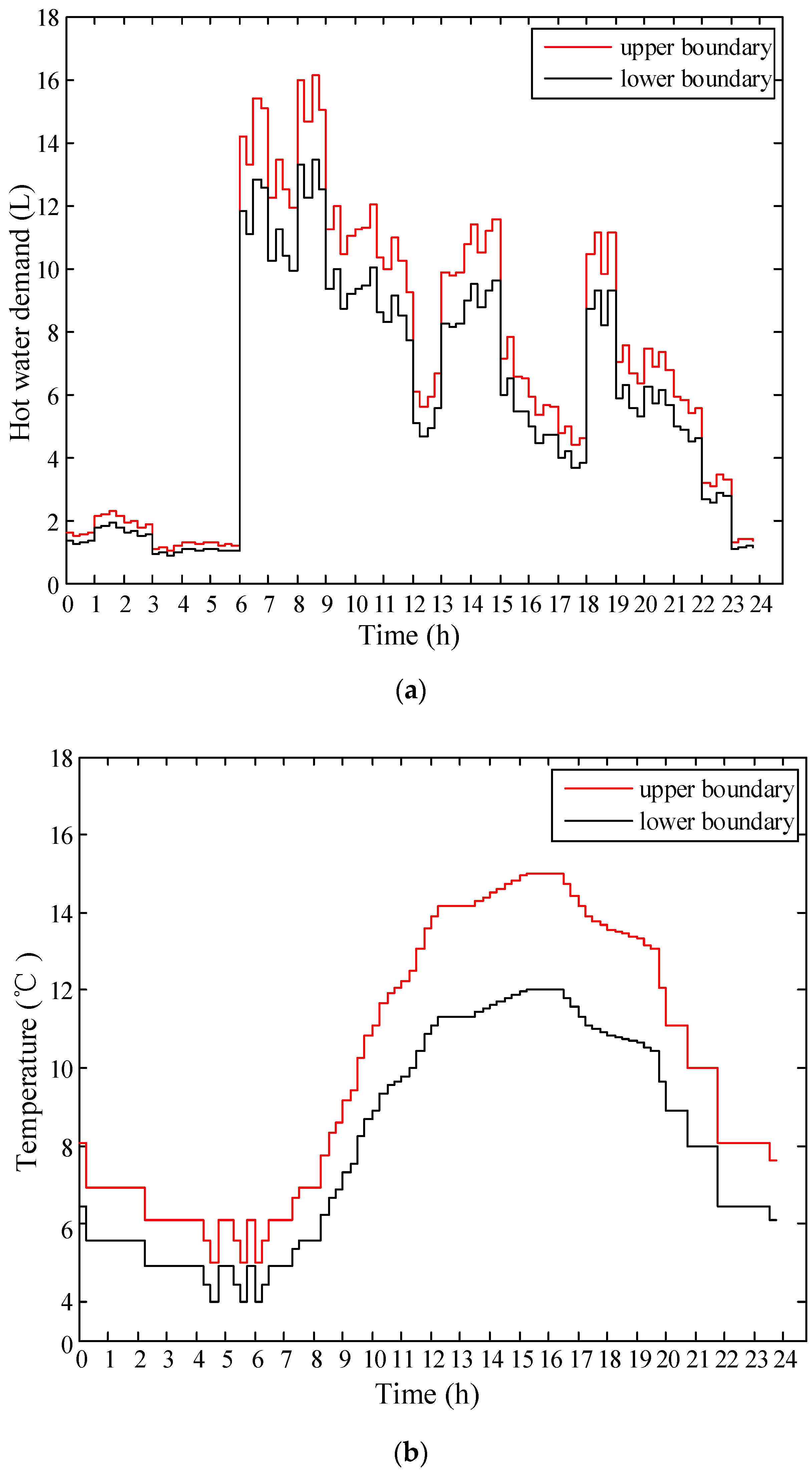
As mentioned above, the uncertain water demand and ambient temperature are transformed into intervals, and the consumers quantify the optimistic degree of the uncertainties by means of setting the robust levels and . In this paper, the forecast maximum intervals of hot water demand and ambient temperature for the next day are plotted in Figure 3, respectively, referring to [23]. As for the maximum values of robust levels, and are both assigned as ten, which denotes that the uncertainties of water demand and ambient temperature are divided into 10 different levels. At the same time, we should think over the deterministic situation where one of the robust levels is equal to zero or both of them are zero. Therefore, the number of the robust level pairs (,) is 11 times 11, being 121 in total.
4.1. The Sscheduling Problem under Different Robust Levels
When consumers believe that the forecast values are highly convincing so that the uncertainties can be ignored, the robust level pair takes the value of (0, 0). Thus, the water demand and ambient temperature lose the characteristic of uncertainty and become real numbers. In this case, the optimal schedule is deemed to be solved without uncertainties, called “deterministic schedule” for convenience. However, in practice, the uncertainties of hot water demand and ambient temperature actually give rise to huge fluctuations of the water temperature in tank, so it is possible that the huge fluctuations may make the water temperature out of the threshold when applying the deterministic schedule.
Therefore, it is necessary to make a sensitivity analysis to figure out the influence of these uncertainties. As stated in Section 3.1, the robust parameters somehow indicate the different uncertainty levels of the parameters, therefore that are used here to generate the various scenarios that are used to verify the deterministic schedule. Specifically, the robust parameters are both set from zero to ten, creating 121 scenarios of different water demand and ambient temperature values. While still applying the deterministic schedule, the actual hot water temperatures in the 121 scenarios are shown in Figure 4.
In Figure 4, the red line represents the upper boundary of the actual water temperature in tank. However, the 121 different sorts of blue lines represent different lower boundaries, while robust level pairs are set from (0, 0) to (10, 10). Specially, the special line colored black is exactly the lower boundary of water temperature under the highest level of uncertainties, where the values of two robust levels both are 10. As shown in Figure 4, from 8 a.m. to 12 p.m., most blue lines are lower than the consumers’ lower threshold line, which means that the thermal comfort constraints are violated. This fact demonstrates that the deterministic schedule cannot satisfy the consumers’ thermal comfort requirement under most levels of uncertainties and in most times of a day. The minimum water temperature is down to 48.53 °C, and the difference between the minimum value and the threshold reaches 6.47 °C. Such a great temperature deviation is unacceptable for common people.
To evaluate the degrees of the violation of the constraints under crossed impact of the two parameters, average differences of water temperature between the lower boundaries and threshold are shown in Figure 5. Obviously, with the uncertainty levels of the two parameters increasing, the average temperature difference rises more and more seriously. Also, it is easy to find that the robust level, , brings much more dangerous degree of violation than the robust level . That is to say, the hot water demand will create more negative drop on the water temperature than the ambient temperature. In one word, the aforementioned the DEWH load scheduling model with different robust levels is indispensable for the consumers to obtain robust solutions.
4.2. Robust Schedules with Different Robust Levels
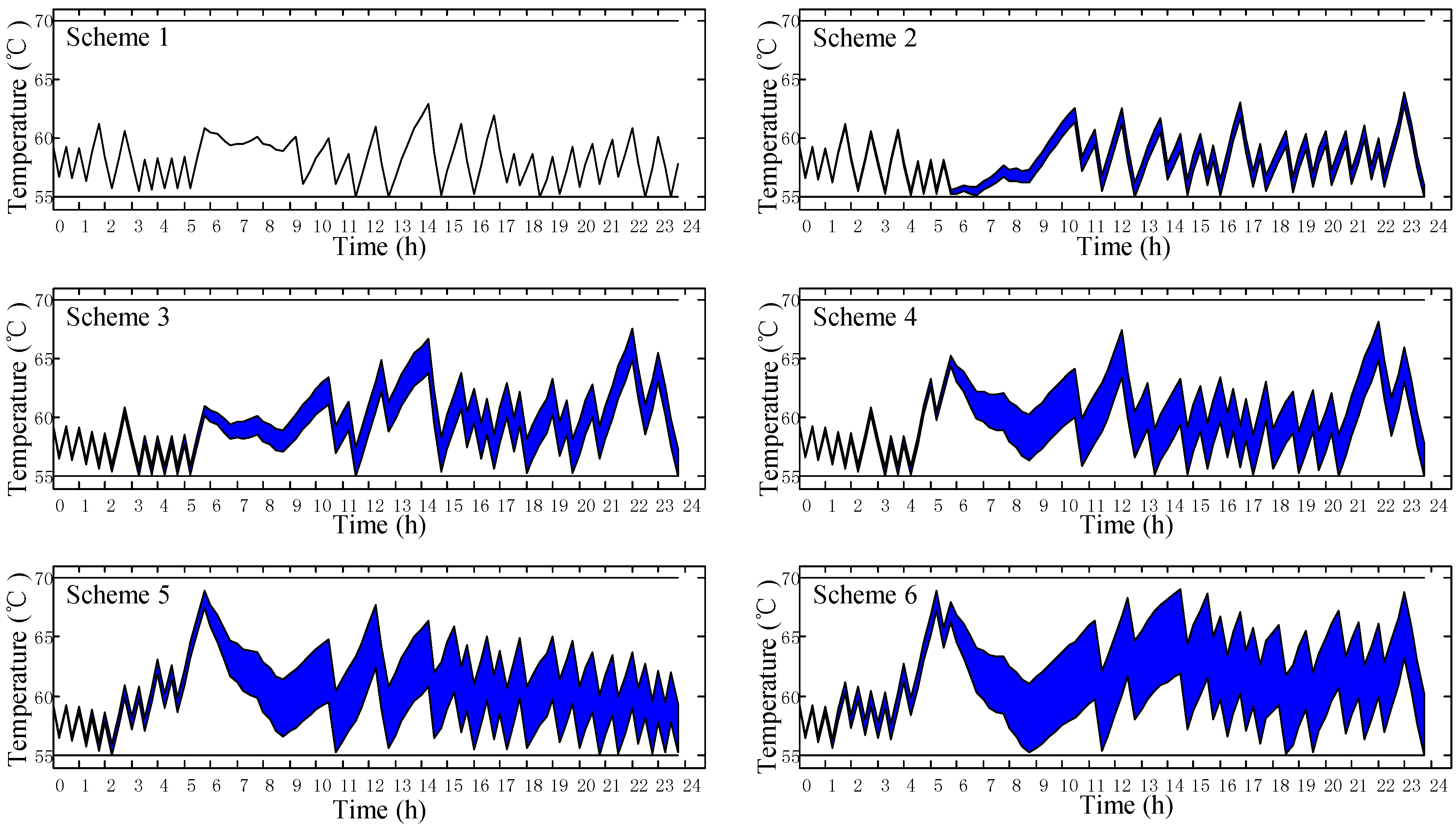
In this part, the load schedules with different robust levels and the corresponding electricity payment are presented. The various robust schemes are solved by CPLEX under difference levels of uncertainties. Six typical robust schemes, where the robust level pairs (,) are set as (0, 0), (2, 2), (2, 8), (8, 2), (8, 8), and (10, 10), respectively, are extracted from the 121 robust schemes as representatives and are shown in Figure 6. It can be seen that all of the typical schemes strictly satisfy the users’ comfort constraints under corresponding uncertain levels. It demonstrates the great robustness of the schemes while facing different levels of uncertainties. As the uncertain levels increasing, the interval of hot water temperature becomes wider.
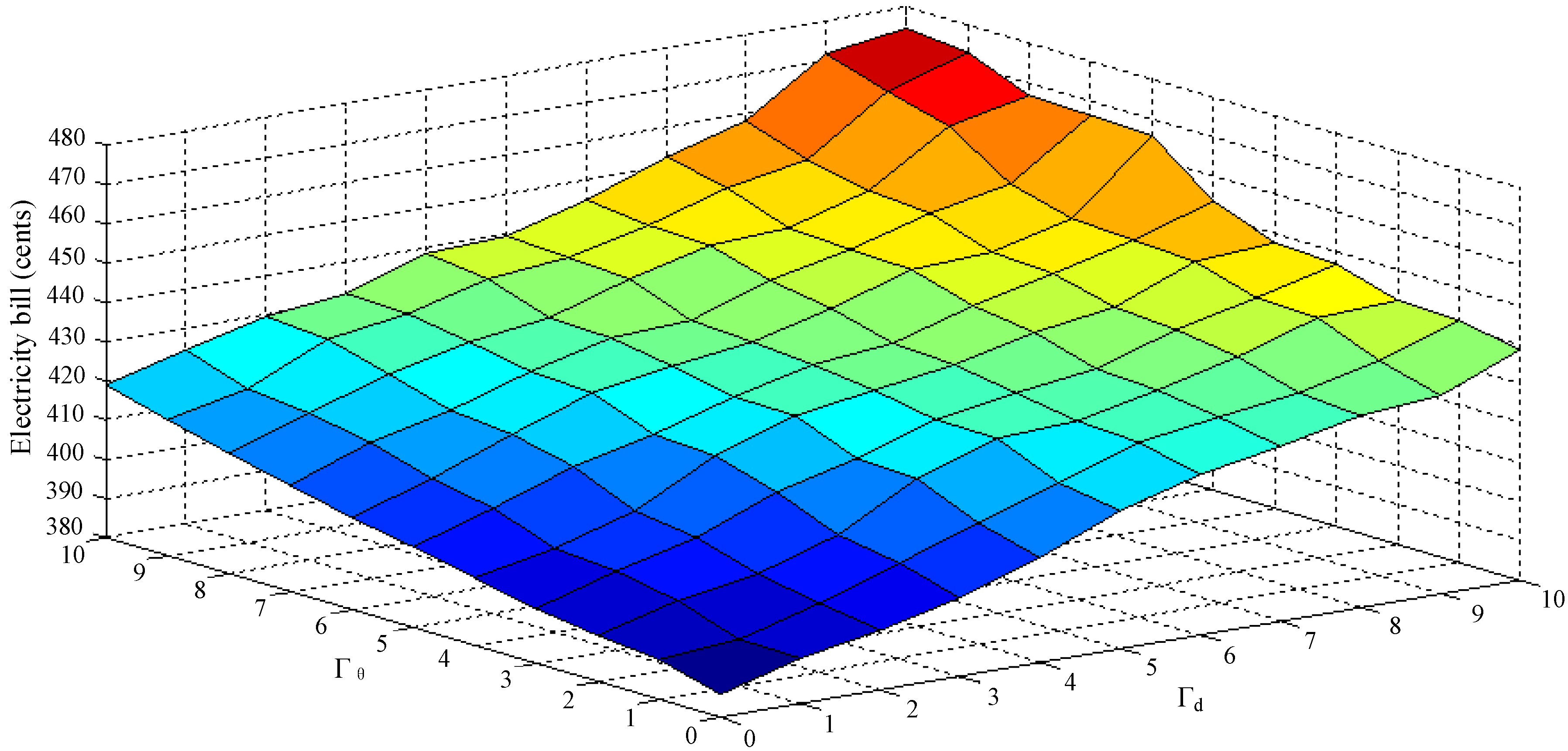
Observing the six schemes in Figure 6 and the RTP prices in Figure 1, the schemes indeed pre-heat the water during the period that the RTP prices are generally low and shut down the DEWH when the prices are extremely high. When compared with the six schemes, it can be found that the working periods with high level of uncertainties are much longer to maintain the temperature in the comfort zone. Figure 7 gives the values of electricity bill under different robust levels settings. As shown in Figure 7, to meet the constraints under higher level of uncertainties, the users have to pay more. It proof that the users can also gain the completely robust and comfortable schemes at the cost of higher electricity bill.
4.3. The Trade-Off Between the Conservatism of Uncertainties and the Economy
From the above analysis, it is obvious that the bill for consumers will be expensive when they are willing to cover high degree of conservatism of uncertainties. Consequently, acquiring one robust schedule that has not only the best economy, but also the highest level of robustness is a troublesome problem. First of all, to tackle this problem, we predefine two types of scenarios: scenario A is taking the conservatism of only one of the uncertain parameters into account, while scenario B considers the conservatism of both uncertain parameters.
In scenario A, the marginal effect indexes (MEI) for the robust level and are defined in Equations (21) and (22), respectively, reflecting the average incremental cost per level of the single uncertain parameter (the water demand or ambient temperature). When calculating the MEI for one robust level, the other robust level should be assumed as a constant. The marginal effect index bars for the robust level and are plotted in Figure 8.
By means of the MEI, consumers can choose a trade-off robust schedule that contains the most conservatism at the lowest cost when one of the robust level is clear. For example, assuming that the robust level is clearly equal to be nine, but the other robust level may be any integer in the interval [5,8]. This assumption is possible, meaning that consumers have complete confidence in the 9th level of uncertainty of the hot water demand, and have hesitation between 5th and 8th level of the uncertainty of ambient temperature. Form the red bars shown in Figure 8b, the MEI has the lowest value when is equal to 6, indicating that it is the best balance between the conservatism of ambient temperature and the economy. Therefore, the robust schedules under the robust parameter pair (6, 9) is recommended to consumers.
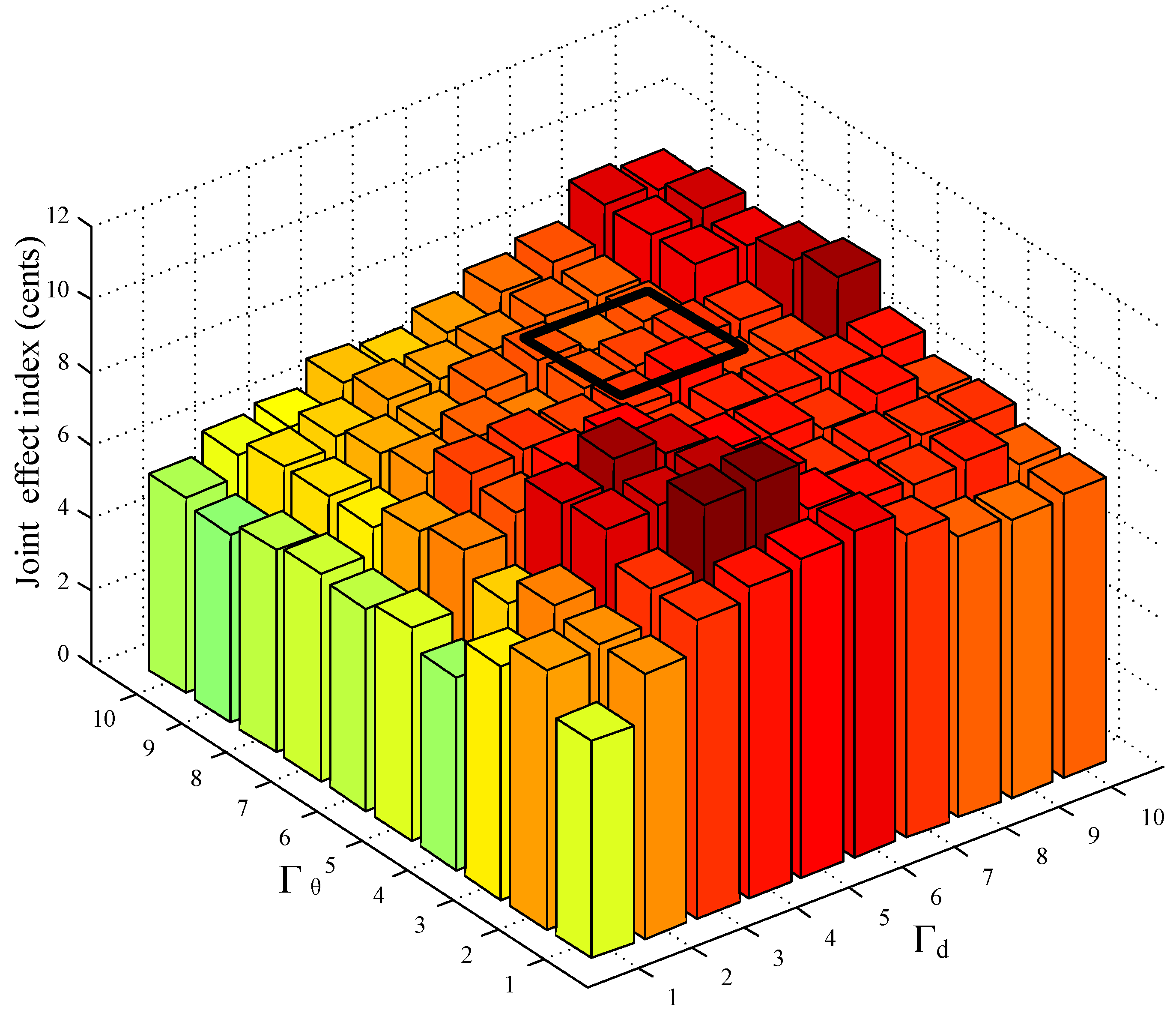
Similarly, the joint effect index (JEI) is defined in Equation (23) to handle the Scenario B. Differing from the single robust level situation in the Scenario A, the root mean square (RMS) of the two robust levels and stands for the per level of the joint impact caused by two uncertain parameters. Just like the MEI, the joint effect index plotted in Figure 9 offers the consumers the most balanced schedule as well. Due to the change of the two robust levels, the bars are only colored for the height of the bars.
Taking another instance for demonstration, we assume that the two robust level and are a integer which is ranged in the interval [6,8]. The black frame in Figure 9 boxes the area where the consumers are not sure about both of the two robust parameters from 6th to 8th level. In this area, the robust level pair (7, 8) has the lowest value and should be offered for consumers.
5. Conclusions
This paper proposes a robust optimization strategy for domestic electric water load scheduling to tackle the uncertainties in the hot water demand and ambient temperature. Specifically, this paper adopts the interval numbers to describe the uncertainties and divided the uncertainties into different robust levels in order to control the degree of the conservatism. By bringing the intervals and robust levels into the constraints, the optimization problem is rebuilt to consider the parameter uncertainties. Furthermore, for easy solving, the constraints that contain the uncertainties are transformed into equivalent deterministic ones. A sensitivity analysis is developed, showing that the infeasibility of the deterministic schedule under various levels of uncertainties.
Simulation results verify that the consumers can obtain various completely robust schemes, which strictly meet the constraints under different levels of uncertainties. Meanwhile, this paper defines the marginal effect index (MEI) and joint effect index (JEI) to evaluate the trade-off between the electricity bill and conservatism of uncertainties. The simulation results indicate that, with the help of the MEI and JEI, the optimal schedule that covers the highest degree of conservatism at the lowest cost is recommended to users.
The proposed robust optimization strategy can be used in home energy management system (HEMS) to help consumers to arrange the DEWH load while facing the uncertainties. Also, it could be applied to more appliances in the future. Moreover, this paper only deals with day-ahead scheduling. The real-time scheduling using the proposed method remains to be studied.
Acknowledgments
The authors greatly acknowledge the support from National Natural Science Foundation of China (NSFC) (51477111) and National Key Research and Development Program of China (2016YFB0901102).
Author Contributions
Jidong Wang contributed to model establishing and paper writing. Many ideas on the paper are suggested by Yingchen Shi to support the work, and Shi did the job of performing the simulations. Kaijie Fang and Yinqi Li analyzed the data. Yue Zhou reviewed the work and modified the paper. In general, all authors cooperated as hard as possible during all progress of the research.
Conflicts of Interest
The authors declare no conflict of interest.
Appendix A
The detailed derivation of Equation (3) is presented as follow: Combining the Equations (1) and (2), there is
To make this expression simpler, we set that
After bringing the simple expression into the Equation (A1), there is
Similarly, in order to make the Equation (A3) shorter, we set that
After that, there is
Hence, the Equation (3) holds.
Appendix B
The detailed derivation of Equation (18) is presented as follow: We use the arithmetic operation rules of interval numbers in the proof progress. Therefore, the basic operation rules between interval numbers are introduced first.
For arbitrary which subject to , , , the rules for interval addition, subtraction, multiplication and division are:
Also, in order to make the expression simpler, we set
Therefore, after bringing the above formulation into the Equation (A3), we can find that the uncertain hot water temperature is transformed into intervals as follows:
Using the arithmetic operation rules of interval numbers above, equation can be further derived as follows:
Because , , therefore Equation (18) holds as follow:
References
- Rastegar, M.; Fotuhi-Firuzabad, M.; Aminifar, F. Load commitment in a smart home. Appl. Energy 2012, 96, 45–54. [Google Scholar] [CrossRef]
- Datchanamoorthy, S.; Kumar, S.; Ozturk, Y.; Lee, G. Optimal time-of-use pricing for residential load control. In Proceedings of the 2011 IEEE International Conference on Smart Grid Communications (SmartGridComm), Brussels, Belgium, 17–20 October 2011; pp. 375–380. [Google Scholar]
- Behrangrad, M.; Sugihara, H.; Funaki, T. Analyzing the system effects of optimal demand response utilization for reserve procurement and peak clipping. In Proceedings of the IEEE PES General Meeting, Providence, RI, USA, 25–29 July 2010; pp. 1–7. [Google Scholar]
- Sun, H.C.; Huang, Y.C. Optimization of power scheduling for energy management in smart homes. Procedia Eng. 2012, 38, 1822–1827. [Google Scholar] [CrossRef]
- Ha, D.L.; Joumaa, H.; Ploix, S.; Jacomino, M. An optimal approach for electrical management problem in dwellings. Energy Build. 2012, 45, 1–14. [Google Scholar] [CrossRef]
- Wang, C.; Zhou, Y.; Wu, J.; Wang, J.; Zhang, Y.; Wang, D. Robust-index method for household load scheduling considering uncertainties of customer behavior. IEEE Trans. Smart Grid 2015, 6, 1806–1818. [Google Scholar] [CrossRef]
- Kepplinger, P.; Huber, G.; Petrasch, J. Autonomous optimal control for demand side management with resistive domestic hot water heaters using linear optimization. Energy Build. 2015, 100, 50–55. [Google Scholar] [CrossRef]
- U.S. Department of Energy. Energy Star Water Heater Market Profile: Efficiency Sells. Available online: http://www.energystar.gov/ia/partners/prod_develpment/new_specs/downloads/water_heaters/Water_Heater_Market_Profile_2010.pd (accessed on 5 September 2010).
- Iwafune, Y.; Yagita, Y. High-resolution determinant analysis of Japanese residential electricity consumption using home energy management system data. Energy Build. 2016, 116, 274–284. [Google Scholar] [CrossRef]
- Goh, C.H.K.; Apt, J. Consumer Strategies for Controlling Electric Water Heaters under Dynamic Pricing; Working Paper CEIC-04–02; Carnegie Mellon Electricity Industry Center: Pittsburgh, PA, USA, 2004. [Google Scholar]
- Du, P.; Lu, N. Appliance commitment for household load scheduling. IEEE Trans. Smart Grid 2011, 2, 411–419. [Google Scholar] [CrossRef]
- Wang, C.; Zhou, Y.; Wang, J. A novel traversal-and-pruning algorithm for household load scheduling. Appl. Energy 2013, 102, 1430–1438. [Google Scholar] [CrossRef]
- Beaudin, M.; Zareipour, H. Home energy management systems: A review of modelling and complexity. Renew. Sustain. Energy Rev. 2015, 45, 318–335. [Google Scholar] [CrossRef]
- Defourny, B.; Ernst, D.; Wehenkel, L. Multistage stochastic programming: A scenario tree based approach to planning under uncertainty. In Decision Theory Models for Applications in Artificial Intelligence: Concepts and Solutions; Sucar, I., Enrique, L., Eds.; Hershey, IGI Global: Derry Township, PA, USA, 2012; pp. 97–143. [Google Scholar]
- Kleywegt, A.J.; Shapiro, A. Stochastic Optimization. In Handbook of Industrial Engineering: Technology and Operations Management; Salvendy, G., Ed.; John Wiley & Sons, Inc.: Hoboken, NJ, USA, 2007; pp. 2625–2649. [Google Scholar]
- Hong, Y.Y.; Lin, J.K.; Wu, C.P.; Chuang, C.C. Multi-objective air-conditioning control considering fuzzy parameters using immune clonal selection programming. IEEE Trans. Smart Grid 2012, 3, 1603–1610. [Google Scholar] [CrossRef]
- Wu, Z.; Zhang, X.P.; Brandt, J.; Zhou, S.Y.; Li, J.N. Three control approaches for optimized energy flow with home energy management system. IEEE Power Energy Technol. Syst. J. 2015, 2, 21–31. [Google Scholar]
- Lee, S.H.; Wilkins, C.L. A practical approach to appliance load control analysis: A water heater case study. IEEE Power Eng. Rev. 1983, PAS-102, 64. [Google Scholar] [CrossRef]
- Ericson, T. Direct load control of residential water heaters. Energy Policy 2009, 37, 3502–3512. [Google Scholar] [CrossRef]
- Kapsalis, V.; Hadellis, L. Optimal operation scheduling of electric water heaters under dynamic pricing. Sustain. Cities Soc. 2017, 31, 109–121. [Google Scholar]
- Pedrasa, M.A.A.; Spooner, T.D.; Macgill, I.F. Coordinated scheduling of residential distributed energy resources to optimize smart home energy services. IEEE Trans. Smart Grid 2010, 1, 134–143. [Google Scholar] [CrossRef]
- Wang, J.; Li, Y.; Zhou, Y. Interval number optimization for household load scheduling with uncertainty. Energy Build. 2016, 130, 613–624. [Google Scholar] [CrossRef]
- Conejo, A.J.; Morales, J.M.; Baringo, L. Real-time demand response model. IEEE Trans. Smart Grid 2010, 1, 236–242. [Google Scholar] [CrossRef]
- Chen, C.; Wang, J.; Heo, Y.; Kishore, S. MPC-based appliance scheduling for residential building energy management controller. IEEE Trans. Smart Grid 2013, 4, 1401–1410. [Google Scholar] [CrossRef]
- Mohsenian-Rad, A.H.; Leon-Garcia, A. Optimal residential load control with price prediction in real-time electricity pricing environments. IEEE Trans. Smart Grid 2010, 1, 120–133. [Google Scholar] [CrossRef]
- Tasdighi, M.; Ghasemi, H.; Rahimi-Kian, A. Residential microgrid scheduling based on smart meters data and temperature dependent thermal load modeling. IEEE Trans. Smart Grid 2014, 5, 349–357. [Google Scholar] [CrossRef]
- 2012 ASHRAE Handbook—Heating, Ventilating, and Air-Conditioning Systems and Equipment. Available online: http://app.knovel.com/web/search.v?q=2012%20ASHRAE%20Handbook&my_subscription=FALSE&search_type=tech-reference (accessed on 10 October 2012).
Figure 1.
The water temperature curve in a domestic electric water heaters (DEWH) tank.
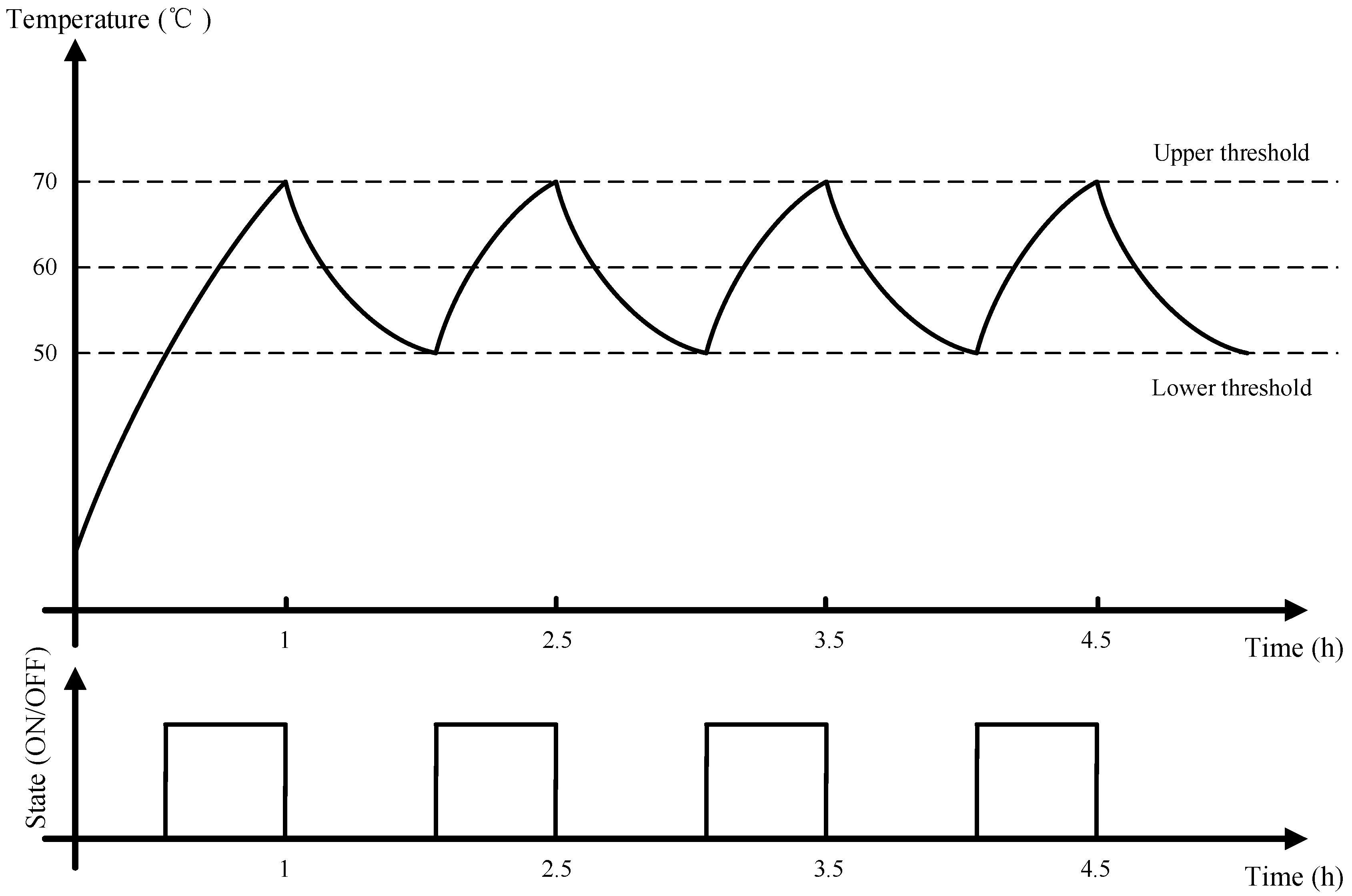
Figure 2.
Real-time pricing (RTP) prices for next day.
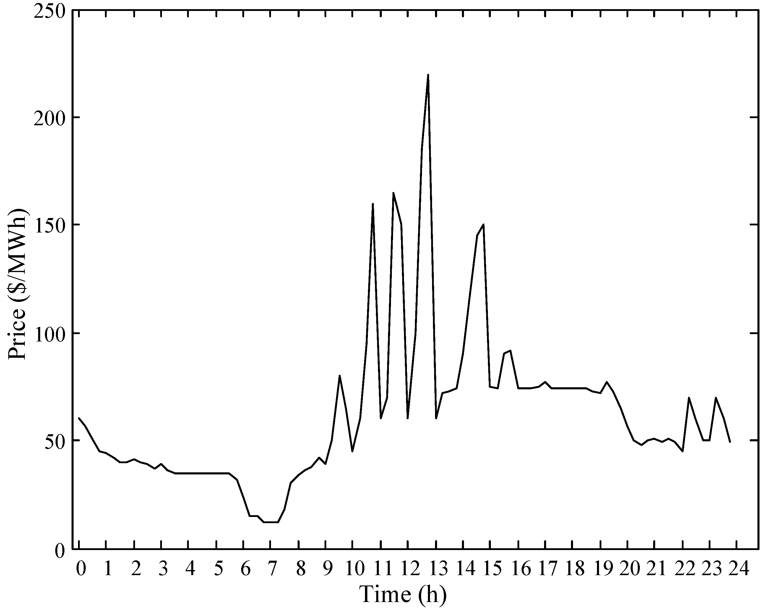
Figure 3.
Maximum forecast intervals for the next day. (a) Hot water demand; (b) Ambient temperature.
Figure 3.
Maximum forecast intervals for the next day. (a) Hot water demand; (b) Ambient temperature.

Figure 4.
The actual water temperature under 121 scenarios applying the deterministic schedule.
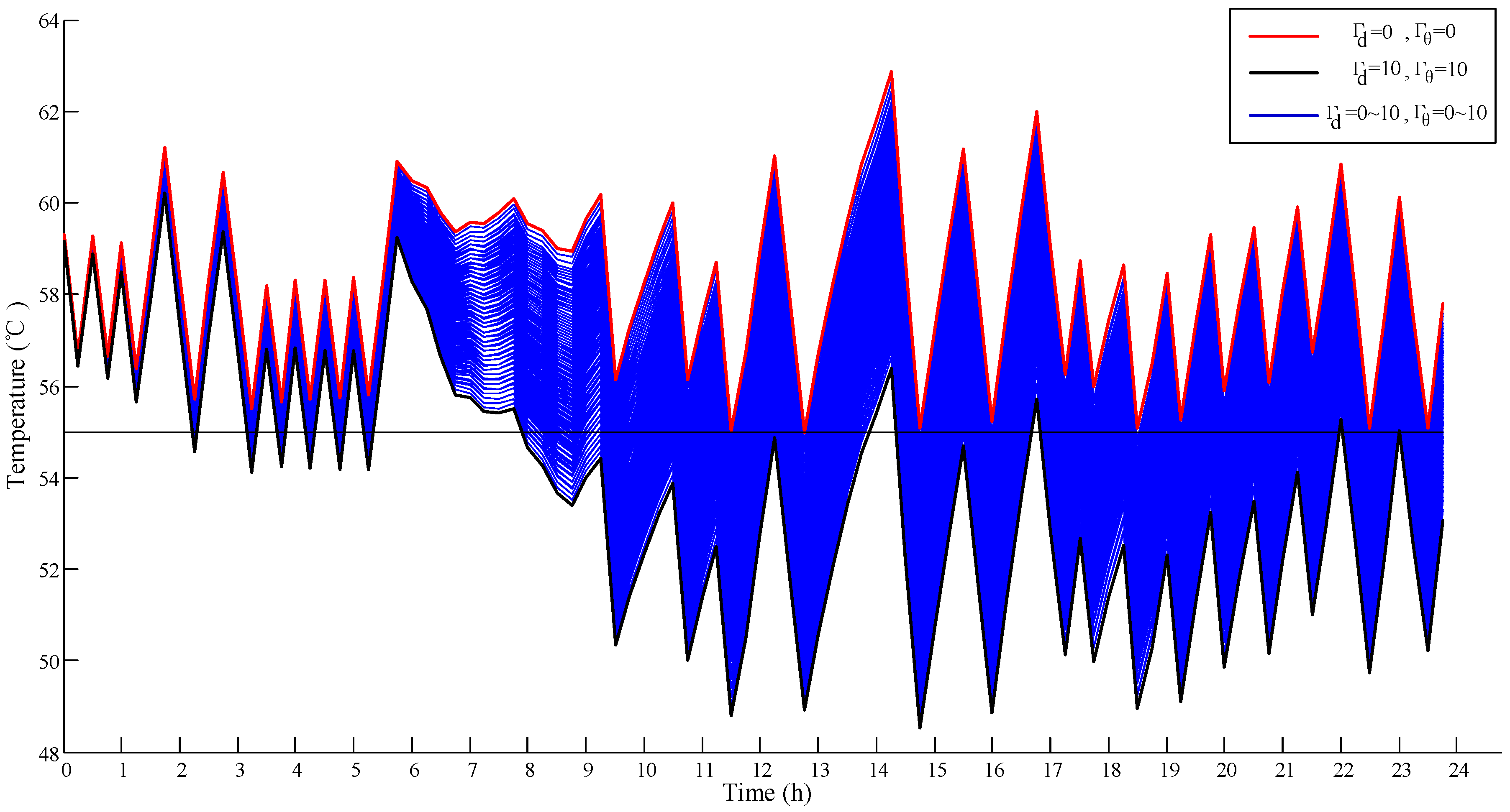
Figure 5.
The average temperature differences under crossed influence the uncertainties.
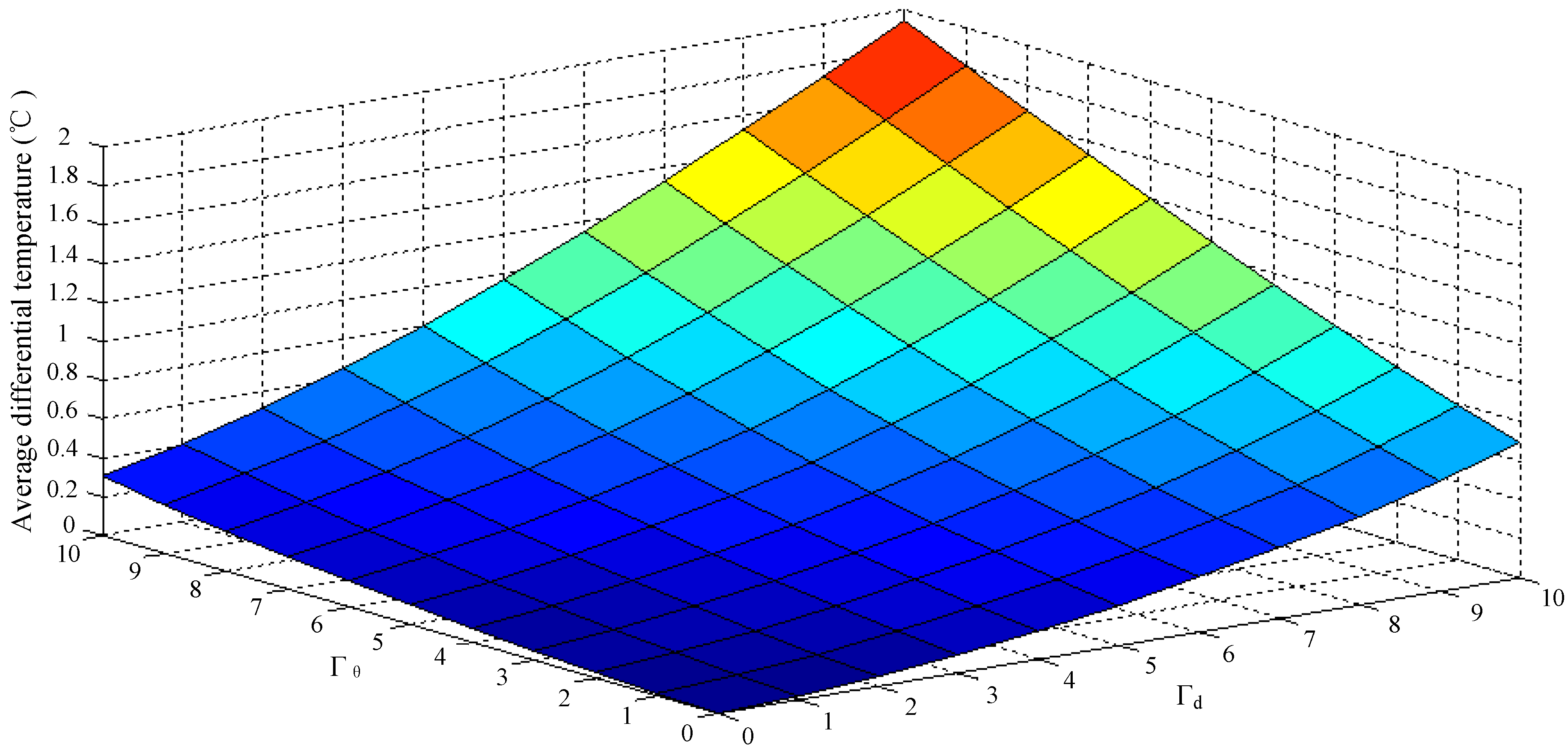
Figure 6.
Hot water temperature under six typical robust schemes.

Figure 7.
The electricity bill under different robust levels.

Figure 8.
(a) The marginal effect index bars for the robust level under different values of ; (b) the marginal effect index bars for the robust level under different values of .
Figure 8.
(a) The marginal effect index bars for the robust level under different values of ; (b) the marginal effect index bars for the robust level under different values of .
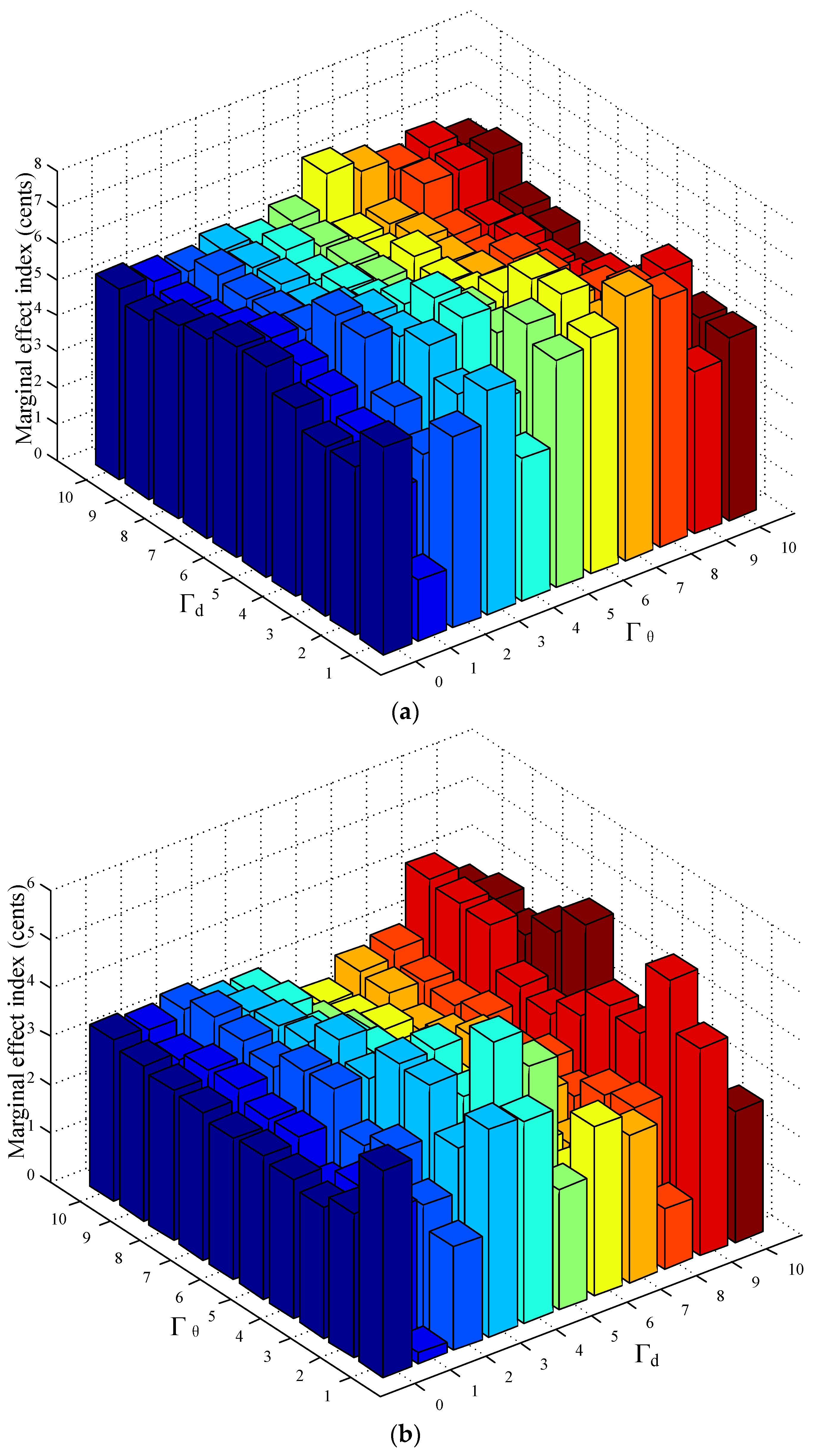
Figure 9.
The joint effect index bars for the two robust level and .


Table 1.
Parameters of the domestic electric water heaters (DEWH).
| 4.5 | 150 | 0.7623 | 431.7012 | 227.1 | 55 | 70 |
© 2017 by the authors. Licensee MDPI, Basel, Switzerland. This article is an open access article distributed under the terms and conditions of the Creative Commons Attribution (CC BY) license (http://creativecommons.org/licenses/by/4.0/).
Share and Cite
MDPI and ACS Style
Wang, J.; Shi, Y.; Fang, K.; Zhou, Y.; Li, Y. A Robust Optimization Strategy for Domestic Electric Water Heater Load Scheduling under Uncertainties. Appl. Sci. 2017, 7, 1136. https://doi.org/10.3390/app7111136
AMA Style
Wang J, Shi Y, Fang K, Zhou Y, Li Y. A Robust Optimization Strategy for Domestic Electric Water Heater Load Scheduling under Uncertainties. Applied Sciences. 2017; 7(11):1136. https://doi.org/10.3390/app7111136
Chicago/Turabian StyleWang, Jidong, Yingchen Shi, Kaijie Fang, Yue Zhou, and Yinqi Li. 2017. "A Robust Optimization Strategy for Domestic Electric Water Heater Load Scheduling under Uncertainties" Applied Sciences 7, no. 11: 1136. https://doi.org/10.3390/app7111136
Note that from the first issue of 2016, this journal uses article numbers instead of page numbers. See further details here.