Simulation of Wind-Battery Microgrid Based on Short-Term Wind Power Forecasting

Abstract

The inherently intermittent and highly variable nature of wind necessitates the use of wind power forecasting tools in order to facilitate the integration of wind turbines in microgrids, among others. In this direction, the present paper describes the development of a short-term wind power forecasting model based on artificial neural network (ANN) clustering, which uses statistical feature parameters in the input vector, as well as an enhanced version of this approach that adjusts the ANN output with the probability of lower misclassification (PLM) method. Moreover, it employs the Monte Carlo simulation to represent the stochastic variation of wind power production and assess the impact of energy management decisions in a residential wind-battery microgrid using the proposed wind power forecasting models. The results indicate that there are significant benefits for the microgrid when compared to the naïve approach that is used for benchmarking purposes, while the PLM adjustment method provides further improvements in terms of forecasting accuracy.

1. Introduction

Microgrids are typically regarded as key building blocks of future power grids, enabling wider deployment of distributed energy resources (DERs) and their effective integration into the main grid [1]. To this end, the Smart Grid concept envisages the use of energy storage for load balancing of decentralized generation units, combined with advanced control and communication technologies, as well as management strategies to improve efficiency, reliability, and the safety of power supply [2]. In this new paradigm, currently passive electricity consumers, such as households and small businesses, can potentially become electricity market agents, also referred to as prosumers, with the ability to produce, consume, and store electricity [3]. Hence, the forecasting accuracy of local production and consumption plays an essential role for successful trading in electricity markets [4].

In this context, prosumers can benefit from real-time monitoring and control over electricity usage in residential or small commercial buildings, where electricity is generated from local micro-renewable energy sources (microRES) and are stored in fixed batteries and/or batteries of plug-in electric vehicles (PHEVs) [5,6]. Despite the challenges for the energy management problem with respect to determining the most beneficial time instance to charge/discharge the fixed and/or PHEV batteries, as well as buy/sell electricity from/to the grid, forecasting the power output from microRES within a certain time frame enables more informed decisions in order to maximize the profit for the prosumer [7].

A typical approach to estimate the power output of a wind turbine consists in matching forecasted wind speed values on the wind turbine power curve. The relevant literature in the field classifies the wind speed forecasting methods into two broad categories, namely physics-based numerical weather prediction models and data-driven approaches [8]. More specifically, the former rely on the physics of the lower atmospheric boundary layer to produce wind flow information, and are thus characterized by high computational complexity [9]. The latter are based on historical wind speed data and employ either statistics-based methods (e.g., time series [10], Kalman filtering [11], Markov chain models [12], and Bayesian methods [13]) or artificial intelligence-based (e.g., artificial neural networks (ANNs) [14], fuzzy systems [15], and support vector machines [16]), or hybrid approaches that combine both techniques to produce wind speed forecasts [17,18,19]. Depending on the intended application, the time scale of wind forecasting can be divided into ultra-short-term (minutes to 1 h ahead), short-term (1 h to several hours ahead), medium-term (several hours to one week ahead), and long-term (one week to more than six months ahead), with respect to the time horizon of the forecasts [20,21].

In general, microgrids can operate either in grid-connected or islanded mode (e.g., in autonomous applications or due to faults in the upstream network), incorporating appropriate control strategies to ensure that the techno-economic requirements for an enhanced energy utilization rate and reduced operating costs are met [22,23]. Given that wind energy is one of the most attractive renewable energy sources (RES) in terms of efficiency and cost-competitiveness, yet it is inherently intermittent and highly variable in nature, the integration of wind turbines in microgrids can be facilitated by the use of energy storage devices in order to counterbalance the potential problems in the reliability and quality of power supply [24]. In [25], an affine projection-like algorithm is proposed to control a wind-diesel microgrid with a battery storage system. In this direction, the work in [26] presents a modified chaos particle swarm optimization approach for the case of a stand-alone microgrid, consisting of photovoltaic, wind turbine, fuel cell, diesel engine, micro-gas turbine, and energy storage. Similarly, the work in [27] considers the optimization of power source capacity in a microgrid with various distributed generators, including wind turbines, and energy storage devices, using a coordinated planning strategy. The authors in [28] examine the problem of optimally sizing battery banks in microgrids with wind power systems, while the study in [29] addresses the problem of optimal placement of energy storage devices in a microgrid to improve the system transient stability. The work in [30] analyzes the performance of a laboratory-scale microgrid with battery banks and hydrogen storage. In [31], a hierarchical approach is introduced for the management of cooperative microgrids and the interaction with the macrogrid. Moreover, the authors in [32] examine the economic impact of integrating PHEVs in microgrids, using a radial basis function network approach to forecast the photovoltaic power output, as well as Monte Carlo simulation to tackle the uncertainties of input parameters. In [33], a stochastic programming formulation is described for the 24-h scheduling problem in a microgrid using combined heat and power, where wind speed forecasting is based on autoregressive-moving-average models.

When combining all of the above, it becomes clear that accurate wind power forecasts are particularly important not only for reducing energy storage requirements and operation costs, but also for participating in the short-term electricity market. Moreover, the adoption of market-based electricity prices provides new opportunities to recoup losses of net revenue and introduces new financial incentives, taking advantage of the electricity storage during peak demand when prices rise and buying electricity from the grid during off-peak periods.

The present work examines the impact of energy management decisions on the performance of a grid-connected microgrid, consisting of a residential building, three wind turbines, and a storage unit, under different short-term wind power forecasting techniques. Specifically, three scenarios are considered with respect to the wind power forecasts: (a) a naïve approach based on the previous value of produced wind power; (b) an ANN clustering approach using statistical feature parameters in the input vector, as a means of striking a reasonable balance between forecasting accuracy, data requirements, and computational complexity [34,35]; and, (c) the previous ANN approach, adjusted by the probability of lower misclassification (PLM) method in order to provide a more realistic value of the expected wind power, and thus reduce the negative effects of forecast errors over electricity utilization, battery storage, and trading with the electricity market [36,37]. In each case, the Monte Carlo simulation is employed to assess the impact of energy management decisions in the residential microgrid, with the aim to reduce the cost of electricity for the building by optimizing the electricity exchanges with the grid and the energy stored in the battery bank. In this context, the main contribution of this work is the introduction of the misclassification probability as a control method in order to reduce the wind power forecasting errors, and by extension, to enhance the energy management decisions for more cost-effective operation of the microgrid.

The rest of this paper is organized as follows: Section 2 describes the methodological approach to model the system components; Section 3 presents the simulation study and discusses the results obtained, while the last section concludes this work.

2. Modeling of System Components

2.1. Modeling of Wind Generator

In general, the performance of a wind turbine is characterized by the power output curve, which is typically employed to estimate the electric output as a function of the wind speed at hub height. The approaches for modeling the wind turbine power curve can be broadly classified into parametric and non-parametric techniques [38,39,40]. The former include piecewise linear functions [41,42,43] and polynomial expressions [44], as well as models that are based on logistic functions with four or five parameters [38,45], while the latter include ANNs [46], fuzzy logic methods [47], and data mining methods [45].

The ideal aerodynamic system model to describe the mechanical output power of the wind turbine is given below:

$$P_{w,I}\left(v\right)=\frac{1}{2}\rho ·A·C_p\left(\lambda ,\beta \right)·v^3,$$

(1)

where P_w,I is the theoretical power that is captured by the rotor of the wind turbine, v is the wind speed, ρ is the air density, A is the swept area of the rotor, and C_p(λ, β) is the dimensionless power coefficient as a function of the tip speed ratio λ and blade angle β. Taking into account that the wind speed near to the ground varies with height, the wind speed v at hub height h is adjusted as follows:

$$v=v_0{\left(h/h_0\right)}^{\alpha },$$

(2)

where v₀ is the reference wind speed at height h₀ and the power law exponent α denotes the ground surface friction coefficient which depends on the roughness of the terrain.

In this work, the wind generator power output is approximated by interpolating the data provided by the manufacturer. The fitting equation of the output characteristic of the wind turbine is described by a sigmoid curve that can be expressed as follows:

$$P_w(v)=\{\begin{array}{c}0\\ A+\frac{B-A}{1+\exp ((C-v)/D)}\\ 0\end{array}\begin{array}{c}0\le v\le v_{ci}\\ v_{ci}\le v\le v_{co}\\ v_{co}\le v\end{array},$$

(3)

where P_w(v) is the output power of the wind generator at wind speed v, while v_ci and v_co are the cut-in and cut-out speeds, respectively, A and B are the horizontal asymptotes, C refers to the inflection point of the curve, and D is the scale parameter.

2.2. Modeling of Storage Battery Operation

As already pointed out, the use of energy storage not only provides a means of counterbalancing the potential problems in reliability and quality of power supply from the fluctuating energy flow of the wind generators in the microgrid, but also enables more cost-effective energy management decisions. The state of the battery (in terms of energy stored) at any time, t, depends on the previous state of charge (SoC) and the energy production/consumption in between. During the charging process, i.e., when the total energy generated by the wind generators is greater than the energy needed by the load, the remaining capacity of the battery E_b(t) at time t is described by the following dynamic equation [23]:

$$E_b\left(t\right)=\left(1-\tau \right)E_b\left(t-1\right)+\left(E_w\left(t\right)-E_L\left(t\right)/{\eta }_D\right)\cdot {\eta }_C,$$

(4)

where τ is the hourly self-discharge rate, E_w(t) is the total energy generated by the wind generators, E_L(t) is the energy consumption of the load, while η_C and η_D are the charge and discharge efficiencies of the battery, respectively. During the discharging process, i.e., when the total energy generated by the wind generators is less than the energy needed by the load, the battery capacity is calculated as follows:

$$E_b\left(t\right)=\left(1-\tau \right)E_b\left(t-1\right)+E_L\left(t\right)/{\eta }_D-E_w\left(t\right).$$

(5)

At any given time t, the remaining capacity of the battery bank is subject to the constraint $E_b^{min}\le E_b\left(t\right)\le E_b^{max}$, where $E_b^{max}$ is the maximum capacity of the battery that corresponds to its nominal capacity C_batt, and $E_b^{min}$ is the minimum capacity of the battery that is determined by the maximum depth of discharge (DoD) provided by the manufacturer as $E_b^{\min }=\left(1-DoD\right)\cdot C_{batt}$.

The net load NL(t) characterizes the total hourly energy balance:

$$NL\left(t\right)=P_L\left(t\right)/{\eta }_D-P_w\left(t\right),$$

(6)

where P_L(t) is the power consumption of the load and P_w(t) is the total power production by the wind turbines [48].

The computation of the net load leads to the following scenarios:

• If NL(t) < 0, there is an excess of production over the demand. In this case, the energy surplus is stored in the batteries until they reach their full capacity. If there is a remainder of available energy, then it is sold to the grid and the new storage capacity is calculated as:

  $$E_b(t+1)=E_b(t)-NL(t)\cdot \Delta t\cdot {\eta }_C,$$

  (7)

  where Δt = 1 h.
• If NL(t) ≥ 0, the load exceeds the production from the wind turbines. In this case, the operational configuration of the system depends on the value of X(t) defined as:

  $$X(t)=NL(t)\cdot \Delta t-{\eta }_D(E_b(t)-E_b^{\min }),$$

  (8)

  where two distinct sub-cases may occur:

• If X(t) > 0, the net load cannot be totally covered by the energy stored in the battery, thus the latter is discharged down to its minimum capacity and the residual demand of value X(t) is bought from the grid. Note that in the case of an isolated system, the value of X(t) would correspond to the loss of power supply.
• If X(t) ≤ 0, the energy stored in the battery can serve the load, thus the new battery capacity is calculated as:

  $$E_b\left(t+1\right)=E_b\left(t\right)-NL\left(t\right)/{\eta }_D.$$

  (9)

2.3. Wind Power Forecasting Model

This work employs an ANN-based approach for 24-h ahead wind power forecasting. The main characteristics of the proposed method include the use of statistical features as input of the multilayer perceptron model, as in [34], along with the consideration of a clustering approach for the output of the network [49]. As a result, an ANN-based clustering model is obtained that classifies the ANN output into power production intervals that are ruled by the power generation curve of the wind turbines (defined in Section 2.1).

The factors forming the input vector I of the ANN are:

$$I=\left[W_{avg},W_{sd},FO{D}_{\max },T_{avg},W_{dir},yd\right],$$

(10)

where W_avg is the average of the wind speed in the last 24 h, W_sd is the standard deviation of the wind speed in the last 24 h, FOD_max is the maximum of the first order difference of the wind speed time series, T_avg is the average of the temperature in the last 24 h, W_dir is the mode of the wind direction in the last 24 h, and yd is the day of the year (yd ∈ [1, 365]) [34]. The statistical parameters W_avg and W_sd in the input vector I represent the dispersion of the wind speed data in relation to the sample mean, while FOD_max provides further information about the variation of the wind speed during the day. Moreover, the parameters T_avg, W_dir, and yd are included in the input vector I to improve the accuracy of the forecasts, as pointed out in [34].

Moreover, the Fisher-Jenks natural breaks optimization method is applied to identify the optimal number of intervals N that classify the power production values based on historical series of wind speed and wind power production [50]. This guarantees that the values of the components of the output vector in Equation (11) fall into one of the Fisher-Jenks intervals.

$$O=\left[O_1,O_2,\dots ,O_{24}\right],$$

(11)

where $O_i\in \left\{C_1,C_2,\dots ,C_N\right\}$ represents the forecasted power class C_i calculated by rounding down the numerical output value of the ANN. The output of the ANN model is a vector of classes that represent the expected power production within the next 24 h. Each class represents an interval that classifies a given value of the power production.

Following the proposed multilayer perceptron architecture in [34], the ANN model employed for the purposes of this work consists of an input layer with six neurons, a hidden layer with 13 neurons, and an output layer of 24 components representing the estimated wind power production in the next 24 h. In addition, the same ANN training method is chosen, namely the Levenberg–Marquardt algorithm.

2.4. Forecast Corrections Using Probability of Misclassification

Similarly to the credit scoring theory that uses the probability of default to measure the uncertainty of a company to meet its debt obligations within a time period [51], this work proposes the use of probability of misclassification to measure the likelihood that the wind turbine output is within the limits of the forecasted power class [52]. Once the ANN model is trained, the confusion matrix M of the N power classes is generated using the test sample. The confusion matrix represents, for each pair of classes {C_i, C_j}, how many predictions from class C_i were incorrectly assigned to power class C_j. Given that the power classes follow an ordered relation as the power output is smaller in the lower classes than in the upper classes, i.e., C₁ < C₂ < … < C_N, only the elements below the diagonal of M have a negative effect on the forecast.

Assuming an n-square confusion matrix A = (a_ij) and its decomposition A = LU, where L = (l_ij) is the lower triangular matrix and U = (u_ij) is the upper triangular matrix, the PLM of matrix M is defined as the vector p = (p_i) with components:

$$p_i=\left({\displaystyle {\sum }_{j=1}^n{l}_{ij}}\right)/\left({\displaystyle {\sum }_{j=1}^n{u}_{ij}}\right).$$

(12)

When considering that the wind speed follows the Weibull distribution [49], the wind turbine power curve is monotonically increasing in accordance with the defined intervals of the power classes, and a large sample (data of approximately one year) is available, it can be assumed without a loss of generality that there is an order-preserving relation between the components of vector p, i.e., p₁ < p₂ < … < p_n (note: the order-preserving relation is not a necessary condition for the proposed method). Interpolating the Fisher-Jenks intervals vector and the vector of PLM, a function describing the probability of negative misclassification of each power class is obtained. This function helps to mitigate the negative effects of a poor rating based on the estimation of wind power, penalizing the upper classes where the risk of misclassification is higher due to the inherent volatility of wind at high speeds, as shown in Figure 1, for the N = 8 power classes obtained by the Fisher-Jenks method.

3. Simulation Study and Discussion of Results

This section analyzes the impact of the proposed short-term wind power forecasting techniques on the performance of the microgrid. To this end, the Monte Carlo simulation is employed to test two different case studies for the daily load demand in the microgrid, namely constant load and fixed (empirical) load curve. For each case study, three scenarios are considered with respect to the wind power forecasts:

• Scenario (a): naive approach (last value of wind power output used as forecast for the next period).
• Scenario (b): ANN-based wind power forecasting model (without PLM correction).
• Scenario (c): ANN-based wind power forecasting model adjusted by the PLM method.

At this point, it is noted that the naive forecasting technique is used as a benchmark for the comparison. Moreover, Monte Carlo simulation is chosen as the method to reflect the stochastic events based on building load demand and wind power production in order to examine the required energy storage at any time [53]. The stochastic variation of wind power production along with the building load demand affect the SoC of the battery, which in turn affects the amount of electricity purchased (or sold) from (or to) the grid. In the context of pricing, the simulation study provides useful insight on the economic efficiency and performance of the system.

3.1. Random Event Generation

The workflow of the proposed Monte Carlo simulation is illustrated in Figure 2. The process begins by loading the input data, including meteorological datasets, wind turbine power curve, ANN model, PLM curve, load profile, battery profile and fixed daily prices. Next, each iteration of the simulation involves the execution of tasks in the following three modules:

• ANN forecasting model: Wind power is estimated using the ANN-based model presented in Section 2.3. In this stage, the initial (unadjusted) wind power forecast for the next 24 h is generated by applying the statistical transformations of the meteorological datasets to the ANN model. This unadjusted forecast is used for scenario (b).
• Misclassification correction: This step is used in the scenario (c) to adjust the wind power forecasts using the PLM method. To simulate misclassified stochastic events, a random binary variable d = (d_i) that follows a binomial distribution with probability p_i is defined, where p_i is the PLM value of the predicted power class at time i. If the value of the random variable d_i is equal to 1, the forecasted power production in period i is considered to be higher than the real power value, and thus it is downgraded by one production class. For example, if the power production of period t was assigned to the power class C5 and the random variable d_i is equal to 1, then the forecast is downgraded to the power class C4. Under these conditions, it is expected that the performance of the system decreases, followed by a decrease in the battery SoC and a potential increase of system costs due to the purchase of extra electricity from the grid. The expected power loss at time t is calculated, in percentage terms, as:

  $$E{L}_i=\max \left(0,d_i\cdot p_i\cdot LGM\right),$$

  (13)

  where LGM is a constant defined as the percentage of power losses given an event of low misclassification. In this case, the output of the ANN model is adjusted by the factor 1-EL in order to calculate the expected power.
• Storage battery operations: The battery operations are simulated taking into account the net load, calculated as the difference between the load demand and power production (the reader is referred to Section 2.2).

3.2. Simulation Output

The output of the Monte Carlo simulation includes in each period: electricity required and produced, average and quantiles of battery SoC, electricity purchased and sold, as well as the cost of economic transactions.

3.3. Description of Dataset

The present work considers that there are three wind turbines and a 1050 Ah storage battery bank that are installed in a residential building. The manufacturer specifications of the wind turbines and battery storage are given in

Table 1. Wind turbine and energy storage specifications.

Description	Specification
Configuration	3 blades, horizontal axis
Rotor diameter	Φ 8.0 m
Rated power	11 kW @ 11 m/s
Cut-in wind speed	3 m/s
Cut-off wind speed	25 m/s
Generator efficiency	>0.85
Battery bank voltage	240 Vdc
System output voltage	110/220 Vac
Wind energy utilizing ratio (Cp)	0.40
Battery voltage	24 V
Battery capacity	150 Ah
Minimum discharge level	30%
Maximum charge level	100%
Battery discharge efficiency	0.8
Battery charge efficiency	0.8

. The dataset consists of 190 days of meteorological samples that are collected at the location of the wind turbines in hourly intervals, with an intensity of wind speed between 0.6 km/h and 16 km/h during the recording period. The main variables under study include hourly averages of wind speed, wind speed standard deviation, wind direction, power generated, temperature, as well as timestamp of the data. The parameter values A = 11,200, B = −400, C = 7.8 and D = 1.46 were used in Equation (3) as the best fit to the manufacturer’s wind turbine power curve, which was divided into eight probability classes using the Fisher-Jenks method.

3.4. Simulation Results and Discussion

Based on the parameters in

Table 2. Parameters of Monte Carlo simulation.

Parameter	Value
Number of iterations	10.000
Simulated days	15
Initial level of battery SoC	80%
Pre-negotiated electricity price: grid to building (G2B)	0.2 €/kWh
Penalized price G2B	0.3 €/kWh
Electricity price: building to grid (B2G)	0.15 €/kWh

, the simulation was executed for a period of 15 days, running 10.000 iterations for each defined scenario. The main variables recorded during the simulation include electricity forecasted, amount of electricity purchased and sold, average battery SoC, trading costs and incomes, as well as total net profit of the system.

3.4.1. Case Study 1—Constant Load Demand

The first case study considers a constant daily load demand curve of 8 kWh during the 15 days of the simulation. Using scenario (a) as a benchmark and the mean absolute percentage error (MAPE) as a measure of error that is applied to each data point of the simulation, a reduction in the forecasting error of 13.8% is observed for scenario (b), and 14.6% for scenario (c), when compared to the value of error (i.e., 26.62%) in the reference scenario (a). This result shows not only the improvements when using the proposed ANN forecasting method, but also the enhancement of the PLM method over the unadjusted ANN-based forecasts.

Examining the distribution of the accuracy of the forecast on a daily basis, it may be observed that 75% of the forecasted values have an absolute error of less than 44.36% in scenario (a), as compared with 16.56% and 15.46% in scenarios (b) and (c), respectively. This result provides an overview of the distribution of forecasting errors during the simulation. Figure 3 depicts the error distribution for the scenarios in case study 1.

Regarding the amount of electricity purchased and sold during the simulations, a substantial difference is observed between scenarios (a) and (b), with an average of 67.59 kWh purchased and 31.97 kWh sold in the scenario (a) versus 49.44 kWh purchased and 42.89 kWh sold in the scenario (b). When comparing scenarios (b) and (c), it is noted that the results of the latter are slightly inferior with an average of 50.46 kWh purchased and 39.01 kWh sold. This observation can be attributed to the fact that, in the PLM method, the minimization of risk dominates the maximization of profits. The same behavior is also observed in the quantiles of electricity that are sold and purchased in scenarios (b) and (c), as shown in

Table 3. Case study 1: Summary of descriptive statistics.

Variable	Scenario	Minimum	1st Quartile	2nd Quartile	Mean	3rd Quartile	Maximum
Electricity purchased (kWh)	(a)	10.60	38.30	72.27	67.59	87.61	127.60
	(b)	0.35	20.60	40.77	49.44	49.48	141.30
	(c)	0.35	25.21	41.24	50.46	79.48	135.50
Electricity sold (kWh)	(a)	0.00	0.00	15.11	31.97	31.33	234.20
	(b)	0.00	0.00	32.57	42.89	55.92	223.30
	(c)	0.00	0.00	31.47	39.01	50.54	218.10
Net profit (€)	(a)	−25.54	−16.97	−10.90	−9.39	−6.03	33.01
	(b)	−28.25	−12.26	−3.26	−3.70	2.11	30.28
	(c)	−27.09	−12.42	−4.01	−4.46	1.17	30.23
Battery charge (Ah)	(a)	444.11	489.04	566.24	583.25	647.91	947.83
	(b)	338.77	538.15	645.38	641.91	703.41	947.89
	(c)	345.76	534.44	638.66	635.49	702.72	939.91

. Analyzing these variables in detail on a daily basis and given that the initial battery SoC is considered as equal to 80%, the simulation results show that the peaks of electricity sales occur during the first and second day of the data sample (note that the first day of the sample refers to a windy day). Figure 4 shows a pyramid diagram of the electricity purchased versus the electricity sold for scenarios (a) and (b).

As far as the costs of electricity purchased and sold are concerned, it is possible to extrapolate the same results that are obtained for the amount of electricity exchanges with few differences revealing the peculiarities of the dataset. In the data sample employed in this work, the wind intensity follows a decreasing pattern during the 15 days of the study, thus rather better results would be expected with a different wind speed pattern. Table 3 also shows the significant improvements in net profit in scenario (a) over (b), as well as the worsening of the results in scenario (c) as compared to (b). Similarly, this is due to the particular characteristics of the sample under study. The PLM-based approach tends to be conservative in order to minimize the risk in the forecast, thus preventing the maximization of profits. The total savings in scenario (b) versus (a) is over 28.56%, while the total savings in scenario (c) as compared to the scenario (a) are slightly lower, i.e., 27.26%.

Regarding the observations of battery usage during the simulation, the comparison of the results in terms of battery charge for scenarios (a)–(c) is not straight-forward as in the previous variables (Table 3). The average battery charge in scenario (a) is significantly lower (by roughly 10%) than that of scenario (b), yet the maximum values of battery charge are almost the same in both of the scenarios. This further implies that the usage of energy storage is less efficient in scenario (a), explaining to a significant extent the lower net profit when compared to scenario (b). Moreover, it is important to note that the maximum battery charge in scenario (c) is slightly lower than scenario (b), implying that there are lower energy storage requirements, as a result of the higher-accuracy wind power forecasts, while maintaining the same average battery usage in both scenarios.

3.4.2. Case Study 2—Fixed Load Curve

The second case study considers a fixed daily load demand curve for the 15 days of the simulation, as given in

Table 4. Case study 2: Fixed daily load demand.

Hour	Daily Load (kWh)	Hour	Daily Load (kWh)	Hour	Daily Load (kWh)
1	6	9	6	17	6
2	3	10	7	18	10
3	2	11	8	19	12
4	2	12	9	20	17
5	2	13	15	21	13
6	2	14	17	22	12
7	2	15	12	23	11
8	5	16	8	24	9

. Following the same approach as in the case study 1, the MAPE value of wind power forecasts remains the same at over 26.62% in the reference scenario (a), while a clear improvement of 12.82% is observed in scenario (b), and even better results in scenario (c) with a MAPE of 12.02%. Regarding the distribution of forecasting accuracy on a daily basis, it is noted that 75% of forecasted values have an absolute error less than 45.36% in scenario (a), when compared with 16.81% in (b) and 15.46% in (c). Figure 5 shows the error distribution for the scenarios in case study 2. These results confirm the benefit from combining the ANN model based on statistical feature parameters with the output adjustment of the proposed PLM method in order to reduce the wind power forecasting errors.

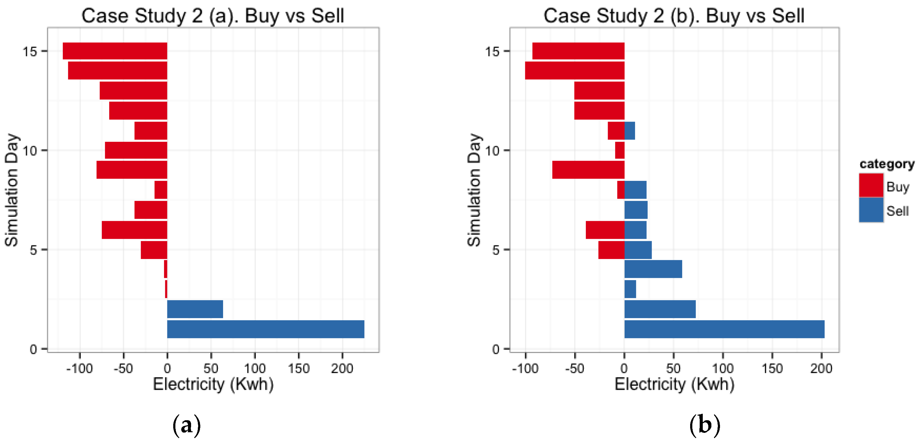
Comparing scenarios (a) and (b), the results in Figure 6 clearly show that the electricity purchased significantly decreases and electricity sold significantly increases in scenario (b), while similar results were observed for scenario (c).

Table 5. Case study 2: Summary of descriptive statistics.

Variable	Scenario	Minimum	1st Quartile	2nd Quartile	Mean	3rd Quartile	Maximum
Electricity purchased (kWh)	(a)	0.00	3.62	38.13	49.10	77.79	120.50
	(b)	0.00	0.00	16.67	31.21	50.29	128.20
	(c)	0.00	0.00	19.79	31.70	51.38	132.50
Electricity sold (kWh)	(a)	0.00	0.00	0.00	19.19	0.00	233.40
	(b)	0.00	0.00	13.37	30.24	29.12	231.80
	(c)	0.00	0.00	10.58	25.38	27.17	223.70
Net profit (€)	(a)	−24.11	−15.56	−9.19	−7.61	−2.12	35.00
	(b)	−25.63	−10.39	−1.31	−1.95	2.92	33.80
	(c)	−26.50	−10.62	−1.53	−2.76	2.23	33.55
Battery charge (Ah)	(a)	315.0	315.0	320.4	448.7	501.9	1003.0
	(b)	315.0	317.5	630.2	649.6	960.7	1013.0
	(c)	315.0	317.2	627.3	637.7	944.8	1013.0

shows a summary of the descriptive statistics that were obtained for case study 2, where it is noted that the results on net profit and battery charge are fully aligned to those of case study 1.

4. Conclusions

This work presents a Monte Carlo simulation study of a residential microgrid in order to assess the potential benefits of introducing the PLM adjustment method in wind power forecasting. The proposed approach, which is inspired by traditional methodologies that are applied to the financing sector, comprises an efficient and practical technique to enhance the quality of wind power forecasts, also reducing the risk under the uncertainty that could result in losses or unexpected expenses. Hence, directions of future work include its implementation on small low-cost devices with limited computational capabilities as components of energy management systems for microgrids.

References

- Ma, X.; Wang, Y.; Qin, J. Generic model of a community-based microgrid integrating wind turbines, photovoltaics and CHP generations. Appl. Energy 2013, 112, 1475–1482. [Google Scholar] [CrossRef]
- Gungor, V.C.; Sahin, D.; Kocak, T.; Ergut, S.; Buccella, C.; Cecati, C.; Hancke, G.P. Smart grid technologies: Communication technologies and standards. IEEE Trans. Ind. Inform. 2011, 7, 529–539. [Google Scholar] [CrossRef]
- Grijalva, S.; Tariq, M.U. Prosumer-based smart grid architecture enables a flat, sustainable electricity industry. In Proceedings of the 2011 IEEE PES Innovative Smart Grid Technologies, ISGT 2011, Anaheim, CA, USA, 17–19 January 2011; pp. 1–6. [Google Scholar] [CrossRef]
- Goncalves Da Silva, P.; Ilic, D.; Karnouskos, S. The Impact of Smart Grid Prosumer Grouping on Forecasting Accuracy and Its Benefits for Local Electricity Market Trading. IEEE Trans. Smart Grid 2014, 5, 402–410. [Google Scholar] [CrossRef]
- Genikomsakis, K.N.; Ioakimidis, C.S.; Eliasstam, H.; Weingraber, R.; Simic, D. A non-myopic approach for a domotic battery management system. In Proceedings of the 39th Annual Conference of the IEEE Industrial Electronics Society, IECON 2013, Vienna, Austria, 10–13 November 2013; pp. 4522–4527. [Google Scholar] [CrossRef]
- Ioakimidis, C.S.; Oliveira, L.J.; Genikomsakis, K.N.; Dallas, P.I. Design, architecture and implementation of a residential energy box management tool in a SmartGrid. Energy 2014, 75, 167–181. [Google Scholar] [CrossRef]
- Ioakimidis, C.S.; Oliveira, L.J.; Genikomsakis, K.N. Wind power forecasting in a residential location as part of the energy box management decision tool. IEEE Trans. Ind. Inform. 2014, 10, 2103–2111. [Google Scholar] [CrossRef]
- Xu, Y.; Dong, Z.Y.; Xu, Z.; Meng, K.; Wong, K.P. An intelligent dynamic security assessment framework for power systems with wind power. IEEE Trans. Ind. Inform. 2012, 8, 995–1003. [Google Scholar] [CrossRef]
- Bhaskar, K.; Singh, S.N. AWNN-Assisted wind power forecasting using feed-forward neural network. IEEE Trans. Sustain. Energy 2012, 3, 306–315. [Google Scholar] [CrossRef]
- El-Fouly, T.H.M.; El-Saadany, E.F.; Salama, M.M.A. One day ahead prediction of wind speed and direction. IEEE Trans. Energy Convers. 2008, 23, 191–201. [Google Scholar] [CrossRef]
- Louka, P.; Galanis, G.; Siebert, N.; Kariniotakis, G.; Katsafados, P.; Pytharoulis, I.; Kallos, G. Improvements in wind speed forecasts for wind power prediction purposes using Kalman filtering. J. Wind Eng. Ind. Aerodyn. 2008, 96, 2348–2362. [Google Scholar] [CrossRef] [Green Version]
- Shamshad, A.; Bawadi, M.A.; Wan Hussin, W.M.A.; Majid, T.A.; Sanusi, S.A.M. First and second order Markov chain models for synthetic generation of wind speed time series. Energy 2005, 30, 693–708. [Google Scholar] [CrossRef]
- Li, G.; Shi, J. Applications of Bayesian methods in wind energy conversion systems. Renew. Energy 2012, 43, 1–8. [Google Scholar] [CrossRef]
- Alexiadis, M.C.; Dokopoulos, P.S.; Sahsamanoglou, H.S. Wind speed and power forecasting based on spatial correlation models. IEEE Trans. Energy Convers. 1999, 14, 836–842. [Google Scholar] [CrossRef]
- Damousis, I.G.; Alexiadis, M.C.; Theocharis, J.B.; Dokopoulos, P.S. A fuzzy model for wind speed prediction and power generation in wind parks using spatial correlation. IEEE Trans. Energy Convers. 2004, 19, 352–361. [Google Scholar] [CrossRef]
- Kramer, O.; Gieseke, F. Short-term wind energy forecasting using support vector regression. Adv. Intell. Soft Comput. 2011, 87, 271–280. [Google Scholar] [CrossRef]
- Hu, J.; Wang, J.; Zeng, G. A hybrid forecasting approach applied to wind speed time series. Renew. Energy 2013, 60, 185–194. [Google Scholar] [CrossRef]
- Liu, D.; Niu, D.; Wang, H.; Fan, L. Short-term wind speed forecasting using wavelet transform and support vector machines optimized by genetic algorithm. Renew. Energy 2014, 62, 592–597. [Google Scholar] [CrossRef]
- Nan, X.; Li, Q.; Qiu, D.; Zhao, Y.; Guo, X. Short-term wind speed syntheses correcting forecasting model and its application. Int. J. Electr. Power Energy Syst. 2013, 49, 264–268. [Google Scholar] [CrossRef]
- Chang, W.-Y. A literature review of wind forecasting methods. J. Power Energy Eng. 2014, 2, 161–168. [Google Scholar] [CrossRef]
- Shao, H.; Deng, X. Short-term wind power forecasting using model structure selection and data fusion techniques. Int. J. Electr. Power Energy Syst. 2016, 83, 79–86. [Google Scholar] [CrossRef]
- Majumder, R.; Ghosh, A.; Ledwich, G.; Zare, F. Power management and power flow control with back-to-back converters in a utility connected microgrid. IEEE Trans. Power Syst. 2010, 25, 821–834. [Google Scholar] [CrossRef] [Green Version]
- Hu, C.; Luo, S.; Li, Z.; Wang, X.; Sun, L. Energy coordinative optimization of wind-storage-load microgrids based on short-term prediction. Energies 2015, 8, 1505–1528. [Google Scholar] [CrossRef]
- Cheng, S.; Sun, W.-B.; Liu, W.-L. Multi-objective configuration optimization of a hybrid energy storage system. Appl. Sci. 2017, 7, 163. [Google Scholar] [CrossRef]
- Pathak, G.; Singh, B.; Panigrahi, B.K. Control of Wind-Diesel Microgrid Using Affine Projection-Like Algorithm. IEEE Trans. Ind. Inform. 2016, 12, 524–531. [Google Scholar] [CrossRef]
- Wang, F.; Zhou, L.; Wang, B.; Wang, Z.; Shafie-khah, M.; Catalão, J.P.S. Modified chaos particle swarm optimization-based optimized operation model for stand-alone CCHP microgrid. Appl. Sci. 2017, 7, 754. [Google Scholar] [CrossRef]
- Liu, Z.; Chen, Y.; Luo, Y.; Zhao, G.; Jin, X. Optimized planning of power source capacity in microgrid, considering combinations of energy storage devices. Appl. Sci. 2016, 6, 416. [Google Scholar] [CrossRef]
- Khorramdel, H.; Aghaei, J.; Khorramdel, B.; Siano, P. Optimal Battery Sizing in Microgrids Using Probabilistic Unit Commitment. IEEE Trans. Ind. Inform. 2016, 12, 834–843. [Google Scholar] [CrossRef]
- Sun, Q.; Huang, B.; Li, D.; Ma, D.; Zhang, Y. Optimal Placement of Energy Storage Devices in Microgrids via Structure Preserving Energy Function. IEEE Trans. Ind. Inform. 2016, 12, 1166–1179. [Google Scholar] [CrossRef]
- Valverde, L.; Rosa, F.; Bordons, C. Design, planning and management of a hydrogen-based microgrid. IEEE Trans. Ind. Inform. 2013, 9, 1398–1404. [Google Scholar] [CrossRef]
- Wang, Y.; Mao, S.; Nelms, R.M. On hierarchical power scheduling for the macrogrid and cooperative microgrids. IEEE Trans. Ind. Inform. 2015, 11, 1574–1584. [Google Scholar] [CrossRef]
- Chen, C.; Duan, S. Optimal integration of plug-in hybrid electric vehicles in microgrids. IEEE Trans. Ind. Inform. 2014, 10, 1917–1926. [Google Scholar] [CrossRef]
- Alipour, M.; Mohammadi-Ivatloo, B.; Zare, K. Stochastic Scheduling of Renewable and CHP-Based Microgrids. IEEE Trans. Ind. Inform. 2015, 11, 1049–1058. [Google Scholar] [CrossRef]
- Ioakimidis, C.S.; Genikomsakis, K.N.; Dallas, P.I.; Lopez, S. Short-term wind speed forecasting model based on ANN with statistical feature parameters. In Proceedings of the 41st Annual Conference of the IEEE Industrial Electronics Society, IECON 2015, Yokohama, Japan, 9–12 November 2015; pp. 971–976. [Google Scholar] [CrossRef]
- Yeh, W.-C.; Yeh, Y.-M.; Chang, P.-C.; Ke, Y.-C.; Chung, V. Forecasting wind power in the Mai Liao Wind Farm based on the multi-layer perceptron artificial neural network model with improved simplified swarm optimization. Int. J. Electr. Power Energy Syst. 2014, 55, 741–748. [Google Scholar] [CrossRef]
- Hodge, B.-M.; Milligan, M. Wind power forecasting error distributions over multiple timescales. In Proceedings of the 2011 IEEE Power and Energy Society General Meeting, Detroit, MI, USA, 24–29 July 2011; pp. 1–8. [Google Scholar] [CrossRef]
- Pinson, P.; Chevallier, C.; Kariniotakis, G.N. Trading wind generation from short-term probabilistic forecasts of wind power. IEEE Trans. Power Syst. 2007, 22, 1148–1156. [Google Scholar] [CrossRef] [Green Version]
- Lydia, M.; Selvakumar, A.I.; Kumar, S.S.; Kumar, G.E.P. Advanced algorithms for wind turbine power curve modeling. IEEE Trans. Sustain. Energy 2013, 4, 827–835. [Google Scholar] [CrossRef]
- Lydia, M.; Kumar, S.S.; Selvakumar, A.I.; Prem Kumar, G.E. A comprehensive review on wind turbine power curve modeling techniques. Renew. Sustain. Energy Rev. 2014, 30, 452–460. [Google Scholar] [CrossRef]
- Shokrzadeh, S.; Jafari Jozani, M.; Bibeau, E. Wind turbine power curve modeling using advanced parametric and nonparametric methods. IEEE Trans. Sustain. Energy 2014, 5, 1262–1269. [Google Scholar] [CrossRef]
- Borowy, B.S.; Salameh, Z.M. Methodology for optimally sizing the combination of a battery bank and PV array in a wind/PV hybrid system. IEEE Trans. Energy Convers. 1996, 11, 367–375. [Google Scholar] [CrossRef]
- Lu, L.; Yang, H.; Burnett, J. Investigation on wind power potential on Hong Kong islands—An analysis of wind power and wind turbine characteristics. Renew. Energy 2002, 27, 1–12. [Google Scholar] [CrossRef]
- Khalfallah, M.G.; Koliub, A.M. Suggestions for improving wind turbines power curves. Desalination 2007, 209, 221–229. [Google Scholar] [CrossRef]
- Thapar, V.; Agnihotri, G.; Sethi, V.K. Critical analysis of methods for mathematical modelling of wind turbines. Renew. Energy 2011, 36, 3166–3177. [Google Scholar] [CrossRef]
- Kusiak, A.; Zheng, H.; Song, Z. On-line monitoring of power curves. Renew. Energy 2009, 34, 1487–1493. [Google Scholar] [CrossRef]
- Marvuglia, A.; Messineo, A. Monitoring of wind farms’ power curves using machine learning techniques. Appl. Energy 2012, 98, 574–583. [Google Scholar] [CrossRef]
- Üstüntaş, T.; Şahin, A.D. Wind turbine power curve estimation based on cluster center fuzzy logic modeling. J. Wind Eng. Ind. Aerodyn. 2008, 96, 611–620. [Google Scholar] [CrossRef]
- Hennet, J.C.; Samarakou, M.T. Optimization of a combined wind and solar power plant. Int. J. Energy Res. 1986, 10, 181–188. [Google Scholar] [CrossRef]
- Du, K.L. Clustering: A neural network approach. Neural Netw. 2010, 23, 89–107. [Google Scholar] [CrossRef] [PubMed]
- Jenks, G.F. The data model concept in statistical mapping. Int. Yearb. Cartogr. 1967, 7, 186–190. [Google Scholar]
- Van Gestel, T.; Suykens, J.A.K.; Baesens, B.; Viaene, S.; Vanthienen, J.; Dedene, G.; De Moor, B.; Vandewalle, J. Benchmarking Least Squares Support Vector Machine Classifiers. Mach. Learn. 2004, 54, 5–32. [Google Scholar] [CrossRef]
- Deaves, D.M.; Lines, I.G. On the fitting of low mean windspeed data to the Weibull distribution. J. Wind Eng. Ind. Aerodyn. 1997, 66, 169–178. [Google Scholar] [CrossRef]
- Tan, C.W.; Green, T.C.; Hernandez-Aramburo, C.A. A stochastic simulation of battery sizing for demand shifting and uninterruptible power supply facility. In Proceedings of the 2007 IEEE Power Electronics Specialists Conference, Orlando, FL, USA, 17–21 June 2007; pp. 2607–2613. [Google Scholar] [CrossRef]
Figure 1.
Empirical curve of probability of lower misclassification (PLM): The x-axis shows the power classes obtained by the Fisher–Jenks method and the y-axis shows the probability of the associated lower misclassification.
Figure 2.
Monte Carlo simulation workflow: The simulation is divided into three stages: (1) power output forecast using artificial neural network (ANN); (2) misclassification correction; and, (3) battery storage operations.
Figure 3.
Case study 1: Distribution of wind power forecasting errors in scenarios (a)–(c).
Figure 4.
Case Study 1: Electricity purchased vs. electricity sold in scenarios (a,b). The diagram on the right shows the increase in selling events with respect to the scenario (a).
Figure 5.
Case study 2: Distribution of wind power forecasting errors in scenarios (a)–(c).
Figure 6.
Case study 2: Electricity purchased vs. electricity sold in scenarios (a,b). The diagram on the right shows the increase in selling events with respect to the scenario (a).