Stochastic Unit Commitment of Wind-Integrated Power System Considering Air-Conditioning Loads for Demand Response


1
State Key Laboratory of New Energy Power System, North China Electric Power University, Beijing 102206, China
2
Department of Electrical and Computer Engineering, Baylor University, Waco, TX 76798-7356, USA
*
Author to whom correspondence should be addressed.
Appl. Sci. 2017, 7(11), 1154; https://doi.org/10.3390/app7111154
Submission received: 3 October 2017
/
Revised: 25 October 2017
/
Accepted: 6 November 2017
/
Published: 10 November 2017
Abstract
:As a result of extensive penetration of wind farms into electricity grids, power systems face enormous challenges in daily operation because of the intermittent characteristics of wind energy. In particular, the load peak-valley gap has been dramatically widened in wind energy-integrated power systems. How to quickly and efficiently meet the peak-load demand has become an issue to practitioners. Previous literature has illustrated that the demand response (DR) is an important mechanism to direct customer usage behaviors and reduce the peak load at critical times. This paper introduces air-conditioning loads (ACLs) as a load shedding measure in the DR project. On the basis of the equivalent thermal parameter model for ACLs and the state-queue control method, a compensation cost calculation method for the ACL to shift peak load is proposed. As a result of the fluctuation and uncertainty of wind energy, a two-stage stochastic unit commitment (UC) model is developed to analyze the ACL users’ response in the wind-integrated power system. A simulation study on residential and commercial ACLs has been performed on a 10-generator test system. The results illustrate the feasibility of the proposed stochastic programming strategy and that the system peak load can be effectively reduced through the participation of ACL users in DR projects.
1. Introduction
New energy power generation, particularly wind power generation, has been developed rapidly around the world in recent years because it may offer clean and cost-effective electric energy. According to the description from the U.S. Department of Energy, by 2030, 20% of the state’s electricity could be generated by wind farms [1]. However, wind power outputs are fluctuating and intermittent [2] because of the wind velocity variation. In addition, wind farms would generate more electricity during valley load periods and less electricity during peak-load periods. In terms of the controllability relative to conventional units, wind power outputs are equivalent to a negative load. As a result, the load peak-valley gap has been significantly widened in wind energy-integrated power systems compared to the traditional power system. Such a gap has brought enormous challenges to the reliable operation of power systems [3,4,5]. In order to supply the excessive load during the peak period, many approaches have been proposed. The traditional approach was to set up new power plants with the capability of peak addition, requiring huge capital investment and planning time [6]. A recently proposed approach was to utilize electric energy storages to adjust the peak load [7,8]. With the rapid development of smart grid techniques, demand response (DR) has been gaining acceptance among practitioners as one of the most useful load shedding methods [9,10]. Moreover, DR is also an efficient measure to coordinate the wind power fluctuation.
The DR is described as a resource that originates from the behavior and usage changes of electricity customers in response to rate variations [11] or incentive mechanisms [12]. Generally, there are two types of DR programs: incentive-based and price-based programs. Electric power companies usually carry out incentive-based DR programs to manage the electric load. According to a Federal Energy Regulatory Commission (FERC) report, in the United States, the incentive-based DR programs account for the majority of the total potential peak reduction reported in 2012 [13]. Additionally, direct load control (DLC) has been reported to be one of the most popular methods of incentive-based DR for peak-load shedding. The DLC [14] projects utilize advanced control technology and remote controllers to switch the on/off state of specific appliances during peak-load periods. The direct control objects are usually the thermostatically controlled loads (TCLs) from residential and small commercial customers, such as heating, ventilation, air-conditioning [15,16] and water heaters.
In the past years, the usage of air-conditioning loads (ACLs) has been steadily increasing [17,18]. In China, for example, during peak-load periods in summer, ACLs account for 30–40% of total load [19] in some large cities, such as Beijing and Shanghai. Research also indicates that turning off the air conditioner or changing the temperature setting for a short period of time has little impact on customer comfort [20]. Therefore, the ACL can be viewed as a potential DR resource in reducing the peak load. Many studies have described and modeled the load characteristics and behaviors of ACLs. For instance, Molina-Garciá et al. [21] adopted the Monte Carlo and the Fokker–Planck methods to analyze the probability distribution function of TCLs. Bashash and Fathy [22] utilized thermostat offset signals to control ACLs and used a novel partial differential equation framework to model ACLs. Additionally, Malhamé and Chong [23] used the statistical approach to model the dynamic behavior of aggregated air conditioners. Nonetheless, most of these works were based on statistical approaches, which require a large amount of data to be collected. Our research, by contrast, is based on an equivalent thermal parameter model of the home heating system, which physically describes the relationship between temperature and ACL power output. In [16], DCL was implemented to control centralized TCLs for providing continuous regulation reserves. The authors elaborately described the control logic of the state-queueing model. Our paper follows the control approach in [16] and introduces ACLs as a load shedding measure into power system scheduling.
Unit commitment (UC) is an essential and important topic in daily power system operation. As wind farms have steadily penetrated into power grids, the effect of wind energy on UC has been an important topic, and much research has been conducted on this topic. For example, Schlueter et al. [24] proposed a UC model and algorithm for utilities with a large penetration of wind generation. Ummels et al. [4] examined the influences of wind energy on UC. Furthermore, DR has been presented to cut down the peak load and coordinate the wind power fluctuation for several years. Zhao et al. [25] developed an advanced algorithm for UC that takes wind energy and DR uncertainties into account. Sioshansi [26] used a DR measure though real-time pricing to curtail the rescheduling costs due to wind generation penetration. In summary, most of the previously mentioned research mainly studied the general model of DR, while the models did not take into account the differences in various DR projects. This paper focuses on UC optimization in wind-integrated power systems, which employs ACL to balance the peak load. Furthermore, the coordination of wind power and ACL was studied in our study. We have also adopted stochastic programming, which is one of the popular approaches for solving wind power uncertainty, and developed a two-stage stochastic unit commitment (SUC) model considering DR resources from ACLs and wind power. Our simulation has verified the feasibility of the model and method proposed by this study. Our results show that controlling the usage of ACLs effectively reduces the peak load and increases energy efficiency. As more and more countries begin to carry out the load control project for ACL users, we believe the findings of this study are of great value.
Four major sections follow the introduction. First, a DR model for ACL is developed in Section 2. Then, a two-stage SUC model is proposed in Section 3, and in Section 4, a 10-generator test system is studied to illustrate the proposed optimal scheduling strategy. Finally, a summary and implications for further research are given in Section 5.
2. Demand Response Modeling for ACL
2.1. Thermal Parameter Model for the ACL
Two methods for building the thermal parameter model for ACLs are widely discussed and used in previous research: (1) a modeling method based on equivalent thermal parameters [15,27], and (2) a modeling method based on cooling load calculations [28]. The latter is based on simpler principles but may involve complex calculations and a low degree of preciseness. Hence, we chose to build our model on the basis of equivalent thermal parameters. The models built upon the equivalent thermal parameter method can be further categorized as physically based electrical models [27] and simplified equivalent thermal parameter models [15]. Although the physically based electrical model is more precise, it involves a complex structure and a large number of calculations. Therefore, it is difficult to apply the physically based electrical model in practice on a large scale. This study focuses on how to reduce the peak load by using ACLs as a load shedding measure. In practice, the proposed strategy requires a quick calculation of schedulable capacity of ACLs on the basis of factors such as temperature. Hence, considering the practical application of the proposed strategy, we chose to use the simplified equivalent thermal parameter model.
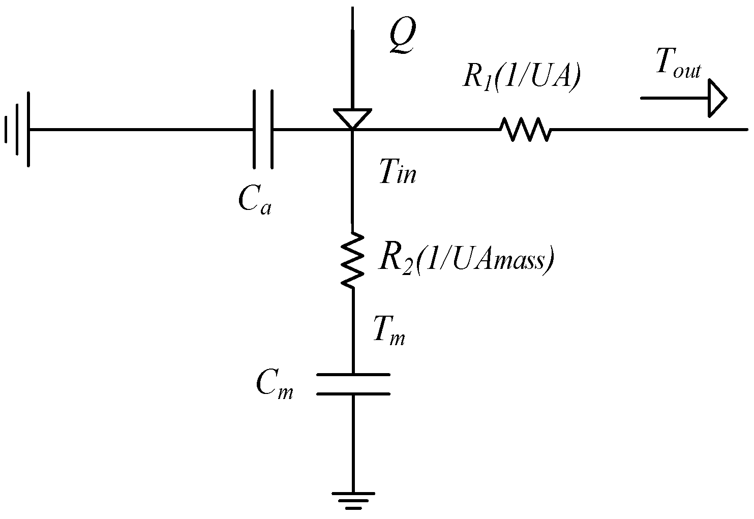
Figure 1 illustrates a simplified equivalent thermal parameter model. This model is applicable to the simulation analysis of the ACL for residential users and small commercial customers. In the figure, Cm is the mass heat capacity; Ca is the air heat capacity; Q is the heat rate; UA is the standby heat loss coefficient, where R1 = 1/UA; UAmass is the standby mass heat loss coefficient, where R2 = 1/UAmass; Tin is the air temperature inside the house; Tout is the ambient temperature; and Tm is the mass temperature inside the house [15].
As simplified from Figure 1, the following dynamic model can be derived for the indoor temperature [15]:
In the model, Tin,t refers to the indoor temperature at time t, Tout,t+1 to the outdoor temperature at time (t + 1), e−Δt/RC to the heat dissipation parameters, Δt to the time interval, R to the equivalent thermal resistance, C to the equivalent thermal capacity, COP to the coefficient of performance, PAC,t to the the ACL power output at time t, A to the conduction coefficient, and SAC to the the switching state of the air conditioner, where “1” and “0” denote the air conditioner being on and off, respectively. In addition, although certain variations might exist in R compared to the uncertainty of wind energy, the uncertainty in R may have a relatively small influence on the simulation results of UC. Hence, in this study, we do not consider the uncertainty in R and assume it as a constant.
2.2. Cost Calculation for the DR of the ACL
Controlling peak load by directing air conditioner usage behaviors can be on the basis of price or incentives. Most of the current research adopts the DLC method to manage the ACL. The DLC is a type of load control method based on the incentive DR. It refers to using smart terminals to directly manage and control a part of the load usage by the dispatching center under the permission of consumers. In return, the customer can receive some compensation. In this paper, the DLC measure has been introduced to control electricity usage of ACL consumers. The detailed control method has been described in [16]. This section primarily provides the cost calculation of using ACLs to cut down peak load on the basis of the above-mentioned method.
The advanced metering technology [29] in the smart grid enables bidirectional communication between the utility operator and the end-user. Therefore, power companies can rely on the infrastructures of the smart grid to dynamically direct consumers’ electricity usage behaviors. It is assumed that every air conditioner is installed with a smart controller. The smart controller can send information to the power company, and when the smart controllers receive a load reduction signal sent from the power company, they will adjust the ACL consumption to reduce the load. At the same time, the income of the power company will be decreased because of the decreased use of power. In addition, the power company has to provide some compensation to the users. Thus, the cost of using ACLs to cut down peak load is equal to the sum of the DR compensation cost and the lost revenue due to the decrease in the load.
The revenue loss of the power company, ∆Cn,t, after the load reduction is
where λ refers to the electricity price, to the power of the nth-type ACL in the DR program before the load reduction at time t, to the the corresponding power after the load reduction at time t, and PAC,n,t to the load reduction.
The compensation cost is the customer outage cost because of the load reduction. The compensation cost can be calculated as a quadratic function of the load reduction [30]:
where K1 and K2 are the cost coefficients; their values are influenced by the load type.
Thus, the cost CAC,n,t for the DR of the ACL is
Substituting Equations (3) and (4) into Equation (5), the final cost CAC,n,t for the DR of the ACL becomes
2.3. Constraints for the DR of the ACL
In the process of load reduction, the power company should consider consumer comfort, making sure that the indoor temperature is within a comfortable range. It is assumed that the lowest and highest indoor temperatures that the consumers are comfortable with are Tmin and Tmax, respectively; then
Because it is difficult to collect the real-time indoor temperature, the current study adopts the equivalent thermal parameter model of the ACL, transferring the temperature constraints in Equation (7) into a response time constraint. During load control periods x, we assume that the average rated power of the ACL is and that the outdoor temperature in the control cycle is a constant, Tout,x. When a consumer turns off the air conditioner, the indoor temperature will increase as time goes by, until it reaches the highest temperature constraint Tmax. When a consumer turns on the air conditioner, the temperature will decrease as time passes by, until it drops to the lowest temperature constraint. Thus, Equations (1) and (2) can be used to calculate the longest air conditioner off-time period toff and the corresponding longest on-time period ton from the following:
Among the various control methods for the DR of the ACL, this paper adopts the state-queuing method [31], providing the computational method for air-conditioning load shedding.
Assuming that there are NAC types of ACLs in the DR program in a specific area, the nth-type ACL is selected and divided into tc groups, and each group is controlled in turn (shown in Figure 2). If the state time interval Δt is 1 min, then at each moment, there are ton groups of ACLs that are on and toff groups of ACLs that are off in the temperature interval [Tmin, Tmax]. The total number of controlling groups/states is equal to the sum of ton and toff.
Thus, during load control periods x, the largest load reduction of the nth-type ACL is as follows:
where Nn refers to the total number of the nth-type ACLs in the DR program. According to Equations (8) and (9), toff and ton can be calculated; then can be calculated as follows:
The constraints for ACLs are that the load shedding PAC,n,t of the nth ACL during load control periods x should not be higher than the largest load shedding:
The power of ACLs is normally determined by the outdoor temperature and the set value of the indoor temperature. This study aims to reduce the peak loads by controlling the usage of ACLs. During peak-load periods, the system sends a load reduction signal to the smart controllers that are connected with the air conditioners. Using the state-queuing method, the smart controllers cyclically control the on/off status of the air conditioners to decrease the ACL and therefore the peak loads.
3. Problem Formulation
3.1. Objective Function
Stochastic programming simulates abundant scenarios to feature variability of random variables. It is an efficient method of solving uncertainties in power system dispatch issues. Most of the current research usually employs a two-stage SUC model to deal with wind power uncertainties. In the two-stage SUC model, the first-stage decision variable is the state of the generation start-up and shutdown. The commitment states of generators are resolved a day ahead on the basis of wind power forecast data. The second-stage decision variables are real-time generation and wind outputs. At the second-stage, numerous wind scenarios are generated as representatives of wind power uncertainties. Subsequently, the real-time economic dispatch in every scenario is solved in this stage on the basis of day-ahead UC from the first-stage. The object is to minimize the sum of the generators’ start-up cost and the generators’ expected operation cost. However, our paper introduces ACLs into the SUC problem and develops a two-stage SUC model considering the DR resource from ACLs and wind power. Thus, the ACL reduction as a decision variable should be considered in the second-stage, and the objective cost should include the expected compensation cost because of the ACL reduction. The objective function is described as follows:
where CUG,i,t refers to the start-up cost of the ith generation unit at time t; CG,i,t,s is the operation cost of the ith generation unit at time t in scenario s; CAC,n,t,s is the cost for the DR of the ACL; gs is the probability of scenario s; NG is the total number of generation units; SG,i,t is the switching state of the ith generation unit at time t, with SG,i,t = 1 for the generation unit being on and SG,i,t = 0 for the generation unit being off; PG,i,t,s is the active power of the ith generation unit at time t in scenario s; ai, bi and ci are the cost coefficients of the ith generation unit, and PAC,n,t,s is the load reduction of the nth-type ACL at time t in scenario s. Equation (14) provides the calculation formula of the operation cost CG,i,t,s of i-th generation unit at time t in scenario s. The quadratic function is typically used to calculate the generators’ operation cost [32]. Equation (15) represents the cost of using the nth-type ACLs to cut down the peak load at time t in scenario s. It follows the same calculation pattern of Equation (6).
Generally, the start-up cost of generators is described by an exponential function. In order to quickly calculate the start-up cost, this can be asymptotically approximated by a stairwise function [32] and formulated as follows:
where KG,i,l refers to the start-up cost of the ith generation unit at the interval l, and NDi is the total number of intervals in the start-up of the ith generation unit.
3.2. Constraints
(1) Minimum up and down time.
For ease of calculation, we need to linearize the minimum up and down time constrains, which are only related to the generators’ commitment states. According to [33], the minimum up and down time constraints can be formulated by the equivalent mixed-integer linear expressions relying on binary variables, which are associated with the different statuses of generating units (e.g., start-up and shutdown). Therefore, the expressions for the minimum up-time constraints can be described as follows:
where refers to the number of initial periods that unit i must be online, = min{T, (TGi,on − TGi,on,0) SG,i,0}, TGi,on is the minimum up-time of the ith generation unit, TGi,on,0 is the time that the ith generation unit has been online, and SG,i,0 is the initial state of the ith generation unit. The constraints in Equation (18) are influenced by the beginning status of the units, which are defined by . The constraints in Equation (19) are used for the following time intervals to meet the requirements of the minimum up-time constraint in all the possible sets of consecutive periods of size TGi,on. The constraints of Equation (20) simulate the last TGi,on − 1 periods in which, if unit i is activated, it is kept online until the end of the time interval.
The minimum down-time constraints are described as follows:
where refers to the number of initial periods that unit i must be offline, = min{T, (TGi,off − TGi,off,0) (1 − SG,i,0)}, TGi,off is the minimum down-time of the ith generation unit, and TGi,off,0 is the time that the ith generation unit has been offline.
(2) The power balance is
where PW,j,t,s refers to the real power of wind power at time t in scenario s, and PL,t to the total system loads at time t.
(3) The generation constraints for the power unit are
where PG,i,min and PG,i,max refer respectively to the upper and lower limits of power from the ith generation unit.
(4) The ramping constraints of the power unit are
where γui and γdi refer to the ramping-up and -down power rates of the ith generation unit, respectively, and T is equal to tc minutes, which is the control cycle for the ACL.
(5) The reserve constraints for the power unit are
where Rt refers to the traditional spinning reserve capacity at time t.
(6) The constraints for the scenario are given by
where PG,i,t,bs is the power of the ith generation unit in the baseline scenario, and ԑi is the spinning reserve capacity of unit i.
(7) The air-conditioning unit constraint is
Our paper selects mixed-integer programming (MIP) to solve the proposed SUC model.
4. Case Study and Simulation Results
We assume that, because of the high temperature of the summer in a specific area, the increased ACL leads to a shortage of electric power. To ensure the stable and secure operation of the power system, the electronic company plans to adopt DR measures for the ACL to shift the peak load. The case study adopted a 10-generator test system. The 24 h load data and wind power data from a specific area were used to conduct a simulation analysis with CPLEX [34] for MATLAB. The parameters of the 10-unit test system can be found in [35].
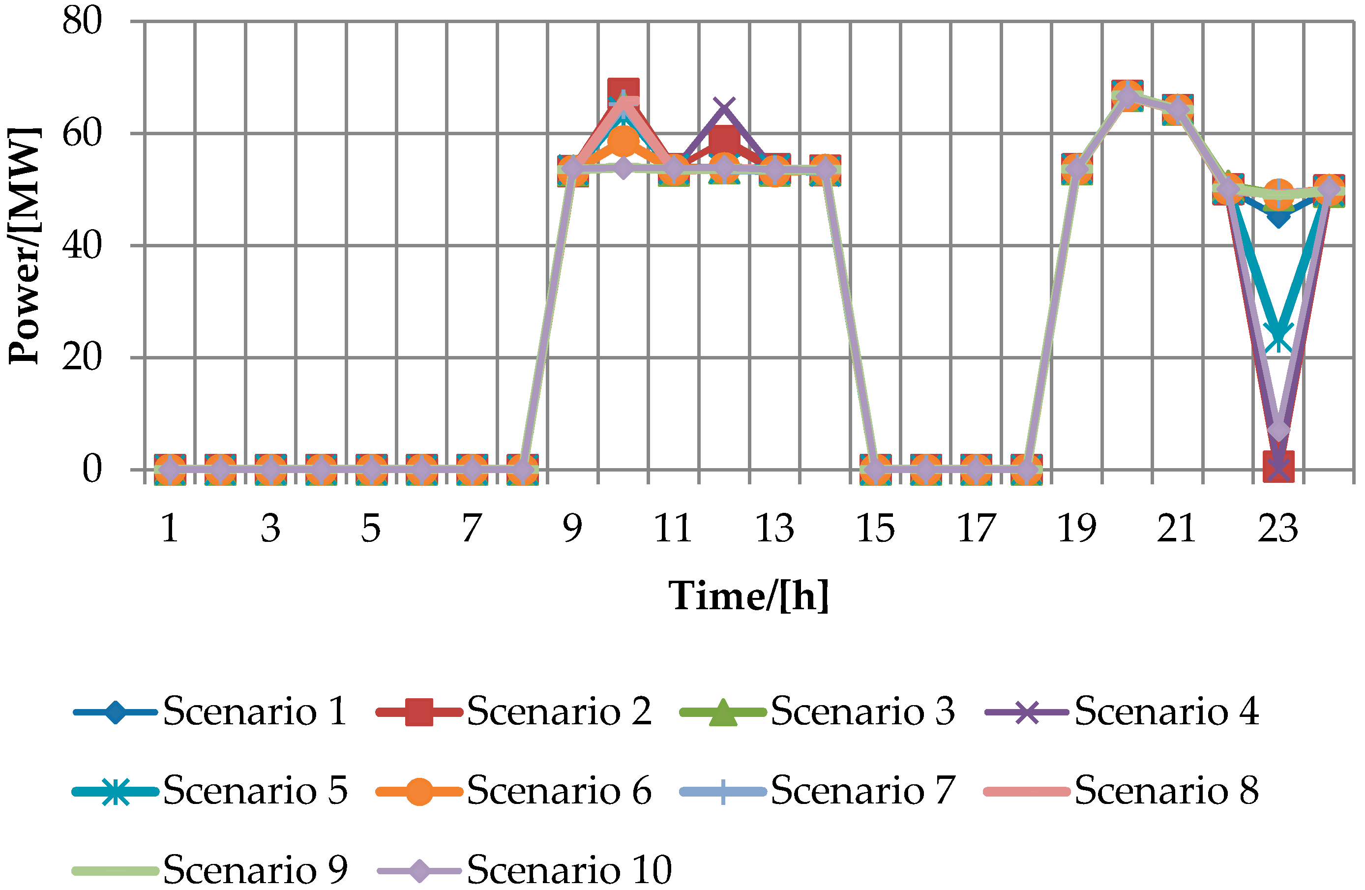
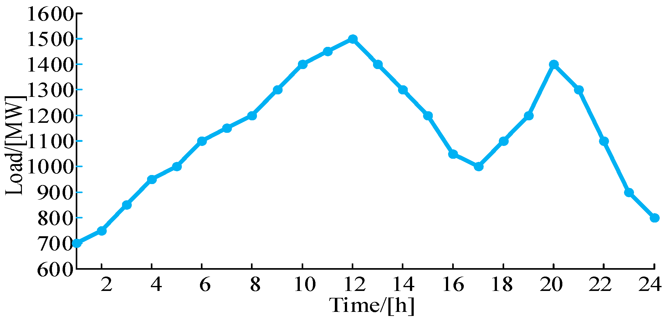
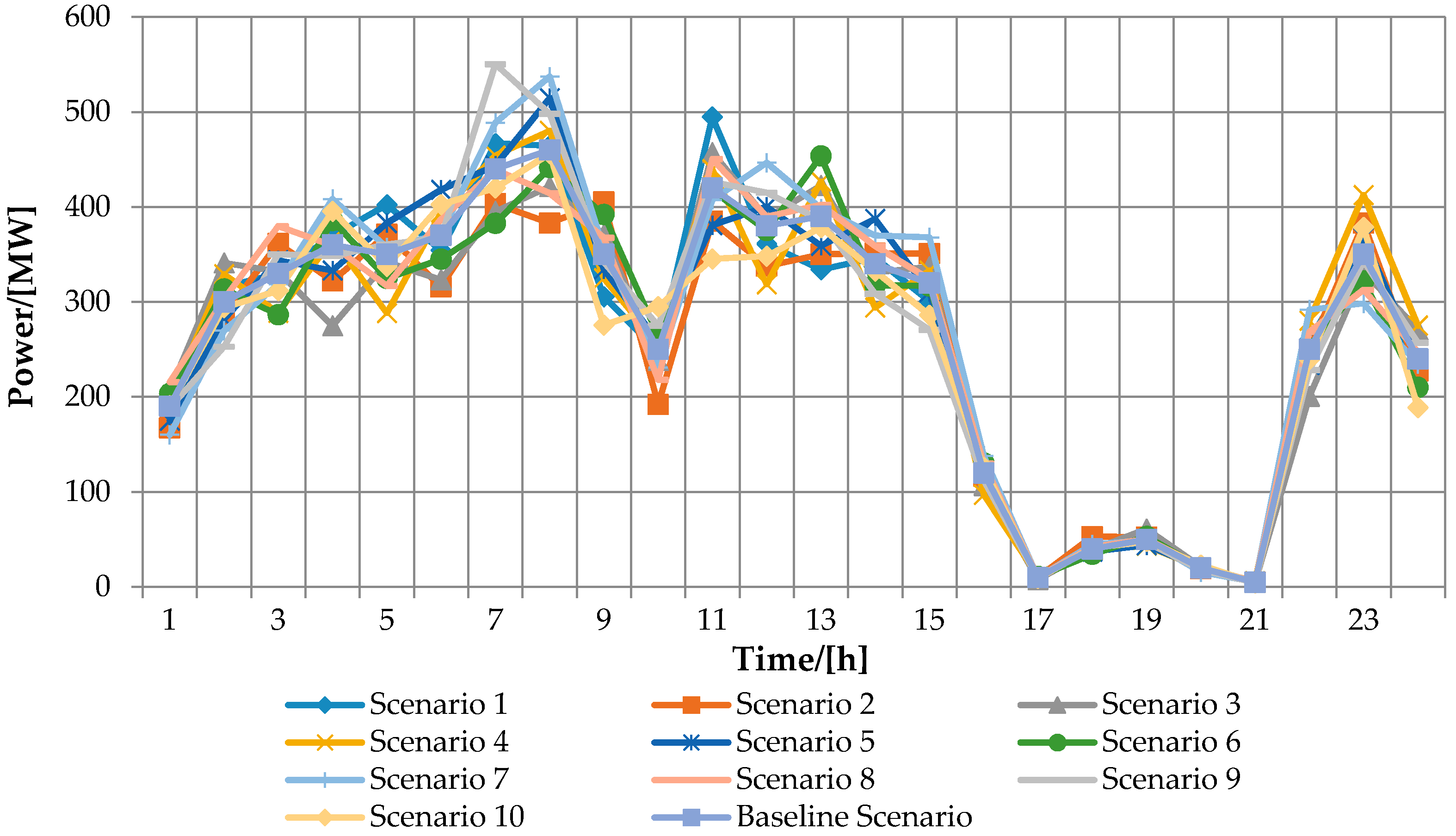
Figure 3 illustrates the initial system load, and Figure 4 shows the wind power of different scenarios as well as the baseline scenario. The methods of generating wind power scenarios and scenario reduction have been described in [36]. Our paper adopted the data of wind power scenarios from [36]. In the high peak period, it is assumed that ACLs account for 30% of the total loads and 15% of the ACL can be included in the power company’s DR program. Thus, 4.5% of the peak load was included in the DR program. In order to ensure the customers’ comfort, we assumed that the indoor temperature was in the range [22 °C, 27 °C]. Figure 5 illustrates the 24 h temperature in summer. Table 1 shows the parameters of the equivalent thermal parameter model.
On the basis of the methods in Section 2, the greatest ACL reduction can be calculated. As shown by Equation (11), the largest ACL reduction will change when the ambient temperature changes. In order to decrease the peak-load demand in Figure 3, we implemented DR for the ACL’s user during peak-load periods. It is assumed that the peak-load periods are during the hours 9–14 h and 19–24 h in the day [35].
The research targets of this paper regard residential and commercial ACLs on a specific area. It is assumed that the weight for each type of ACL in the DR program is 50%. The parameters of the compensation cost for two types of ACL are shown in Table 2.
To investigate the impact of ACLs on UC, a comparison of two modes was simulated. In operation Mode 1, the UT for the wind-integrated power system was optimized without considering the ACL in the DR program. In Mode 2, the UC for the wind-integrated power system was optimized with the ACL. The simulation results of UC in the two modes are shown in Table 3. It can be seen that in Mode 2, the number of units committed was less than that in Mode 1 during the peak periods. In addition, the status of unit 4 at 23 h and unit 6 during the periods 12–14 h and 19–20 h changed from starting to stopping, because of the reduction of the ACL during peak-load periods. Therefore, the model proposed by this study can effectively control the usage of ACL customers during peak-load periods in the afternoon and night, reducing the frequency of unit start–stops and peak loads.
Table 4 provides the cost analysis of the two modes. Both the power generation and start-up costs in Mode 2 were decreased compared to Mode 1, as the participation of ACL users in the DR project decreased the electricity usage during peak-load periods. Hence, the ACL can be regarded as the “virtual power plant” to replace a part of generators. In conclusion, the DR program effectively relieves the excessive peak-load requirement and saves costs for the power company.
Figure 6 illustrates load reduction in Mode 2. The total reduction of the load was 583 MW, accounting for 4% of the peak loads. According to Equation (15), the compensation cost of the ACL is primarily influenced by K1. We also changed the values of K1 under two types of compensation costs of the ACL and compared the impacts of different compensation costs on the load reduction. Figure 7 shows the load reduction results when the values of K1 in the first- and second-type ACL were 1 and 0.9, respectively. Compared to Figure 6, Figure 7 illustrates that the load reduction decreases when the compensation cost is very high. This is because our objective function is composed of the generators’ start-up cost, the generators’ expected operation cost, and the expected compensation cost of the ACL reduction. When the compensation cost is very high, the value of the objective function may be increased. Figure 8 shows the load reduction results when the values of K1 in the first- and second-type ACL were 0.06 and 0.04, respectively. Compared to Figure 6, it shows that when the compensation cost decreases, the system may allocate more ACLs to reduce the peak load. However, the cusomer benefits are decreased. Hence, future research should pay greater attention to how to make a balanced compensation plan from the perspectives of both customers and the electric network.
The front simulation was based on the assumption that 15% of ACL consumers participate in the DR project. With the development of smart grid technology, an increasing number of electricity consumers will join the DR project. Therefore, we analyzed the effect of consumers’ participation on the load reduction. Compared to Figure 6, with the same values of K1 as in the first- and second-type ACL, Figure 9 shows the load curtailment in the case of 25% participation of the ACL consumers. As we can see, more loads are reduced when more ACLs are in the control of the power company.
5. Conclusions
This paper selects ACLs as a DR resource to implement a load reduction during peak-load periods. In order to deal with the uncertainty of wind energy, a two-stage SUC model is developed to analyze the response of ACL users. On the basis of an equivalent thermal parameter model for ACL, this paper proposes a compensation cost calculation method of using ACL to cut down the peak load.
A simulation analysis of the model was conducted in a 10-generator test system, and the validity and practicability of our model were demonstrated. Several implications can be drawn from our simulation analysis. First, ACL shows enormous potential in load shedding. By designing reasonable incentives and compensation policies, ACL users can be motivated to respond towards the DR program, suggesting that the ACL would be an efficient load shedding measure in power system scheduling. Second, compared with the previous UC model of wind-integrated power systems without considering the ACL for DR, the optimization model proposed in this paper (incorporating the DR resources considering ACLs into UC) can effectively reduce peak loads, decrease the operation cost of the system and frequency of unit start–stops, foster efficient interaction between the demand-side and generation-side resource, resolve the tensions between the electronic supply and demand, and therefore lead to the reliable and economical operation of electric power systems. Third, the compensation measure proposed in this paper can largely motivate ACL users to respond towards power system dispatching. Last but not least, when designing reasonable incentives and compensation policies, the electric power company should consider the tradeoffs between customer benefits and the cost of the power system. For instance, if the compensation cost is too high, it might lead to certain uneconomic consequences from the perspective of the system operation. If the compensation cost is too low, customer benefits may be affected. Hence, it is important for the electric power company to take a comprehensive view so as to make an acceptable and valuable plan for both sides.
We recommend certain future study directions on the basis of the simulation results and findings of this study. First, while it involves a complex structure and a large number of calculations, the physically based electrical model may be more precise than the simplified equivalent thermal parameter model. Hence, we suggest that future studies should aim to build models based on the physically based electrical model. Second, with the exception of temperature, the comfort factor may also be affected by other factors such as humidity. Hence, future studies are recommended to include such factors in their proposed model to improve the generalizability and degree of preciseness.
Acknowledgments
This work is supported by the National Natural Science Foundation of China under Grant 51577061.
Author Contributions
The paper was a collaborative effort between the authors. Xiao Han carried out the main research tasks and wrote the full manuscript. Ming Zhou and Gengyin Li provided very helpful suggestions during the whole process. Kwang Y. Lee helped to largely improve the whole manuscript.
Conflicts of Interest
The authors declare no conflict of interest.
References
- U.S. Department of Energy. 20% Wind Energy by 2030: Increasing Wind Energy’s Contribution to U.S. Electricity Supply. Available online: http://energy.gov/eere/wind/wind-program (accessed on 14 May 2016).
- Cheng, S.; Sun, W.B.; Liu, W.L. Multi-objective configuration optimization of a hybrid energy storage system. Appl. Sci. 2017, 7, 163. [Google Scholar] [CrossRef]
- Jiang, R.; Wang, J.; Guan, Y. Robust unit commitment with wind power and pumped storage hydro. IEEE Trans. Power Syst. 2012, 27, 800–810. [Google Scholar] [CrossRef]
- Ummels, B.C.; Gibescu, M.; Pelgrum, E.; Kling, W.L.; Brand, A.J. Impacts of wind power on thermal generation unit commitment and dispatch. IEEE Trans. Energy Convers. 2007, 22, 44–51. [Google Scholar] [CrossRef]
- Bouffard, F.; Galiana, F.D. Stochastic security for operations planning with significant wind power generation. IEEE Trans. Power Syst. 2008, 23, 306–316. [Google Scholar] [CrossRef]
- Babu, C.A.; Ashok, S. Peak load management in electrolytic process industries. IEEE Trans. Power Syst. 2008, 23, 399–405. [Google Scholar] [CrossRef]
- Linden, S.V.D. Bulk energy storage potential in the USA, current developments and future prospects. Energy 2006, 31, 3446–3457. [Google Scholar] [CrossRef]
- Zhao, P.; Wang, J.; Dai, Y. Capacity allocation of a hybrid energy storage system for power system peak shaving at high wind power penetration level. Renew. Energy 2015, 75, 541–549. [Google Scholar] [CrossRef]
- Shao, S.; Pipattanasomporn, M.; Rahman, S. Demand response as a load shaping tool in an intelligent grid with electric vehicles. IEEE Trans. Smart Grid 2011, 2, 624–631. [Google Scholar] [CrossRef]
- Qela, B.; Mouftah, H.T. Peak load curtailment in a smart grid via fuzzy system approach. IEEE Trans. Smart Grid 2014, 5, 761–768. [Google Scholar] [CrossRef]
- Parvania, M.; Fotuhi-Firuzabad, M. Demand response scheduling by stochastic SCUC. IEEE Trans. Smart Grid 2010, 1, 89–98. [Google Scholar] [CrossRef]
- Vahedipour-Dahraie, M.; Najafi, H.; Anvari-Moghaddam, A.; Guerrero, J.M. Study of the effect of time-based rate demand response programs on stochastic day-ahead energy and reserve scheduling in islanded residential microgrids. Appl. Sci. 2017, 7, 378. [Google Scholar] [CrossRef]
- Assessment of Demand Response and Advanced Metering Staff Report (Docket AD06-2-000). Available online: https://www.smartgrid.gov/document/assessment_demand_response_advanced_metering_staff_report_docket_ad06_2_000 (accessed on 4 September 2015).
- Huang, K.Y.; Huang, Y.C. Integrating direct load control with interruptible load management to provide instantaneous reserves for ancillary services. IEEE Trans. Power Syst. 2004, 19, 1626–1634. [Google Scholar] [CrossRef]
- Lu, N. An evaluation of the HVAC load potential for providing load balancing service. IEEE Trans. Smart Grid 2012, 3, 1263–1270. [Google Scholar] [CrossRef]
- Lu, N.; Zhang, Y. Design considerations of a centralized load controller using thermostatically controlled appliances for continuous regulation reserves. IEEE Trans. Smart Grid 2013, 4, 914–921. [Google Scholar] [CrossRef]
- Hassan, N.U.; Khalid, Y.I.; Yuen, C.; Tushar, W. Customer engagement plans for peak load reduction in residential smart grids. IEEE Trans. Smart Grid 2015, 6, 3029–3041. [Google Scholar] [CrossRef]
- Tso, G.K.F.; Yau, K.K.W. A study of domestic energy usage patterns in Hong Kong. Energy 2003, 28, 1671–1682. [Google Scholar] [CrossRef]
- Li, C.; Shang, J.; Zhu, S.; Du, L.; Wu, C.; Wang, Q. An analysis of energy consumption caused by air temperature-affected accumulative effect of the air conditioning load. Autom. Electr. Power Syst. 2010, 34, 30–33. [Google Scholar]
- Horowitz, S.; Mauch, B.; Sowell, F. Forecasting residential air conditioning loads. Appl. Energy 2014, 132, 47–55. [Google Scholar] [CrossRef]
- Molina-Garcia, A.; Kessler, M.; Fuentes, J.A.; Gomez-Lazaro, E. Probabilistic characterization of thermostatically controlled loads to model the impact of demand response programs. IEEE Trans. Power Syst. 2011, 26, 241–251. [Google Scholar] [CrossRef]
- Bashash, S.; Fathy, H.K. Modeling and control insights into demand-side energy management through setpoint control of thermostatic loads. Am. Control Conf. 2011, 47, 4546–4553. [Google Scholar]
- Malhame, R.; Chong, C.Y. Electric load model synthesis by diffusion approximation of a high-order hybrid-state stochastic system. IEEE Trans. Autom. Control 1985, 30, 854–860. [Google Scholar] [CrossRef]
- Schlueter, R.A.; Park, G.L.; Reddoch, T.W.; Barnes, P.R.; Lawler, J.S. A modified unit commitment and generation control for utilities with large wind generation penetrations. IEEE Power Eng. Rev. 1985, 85, 1630–1636. [Google Scholar]
- Zhao, C.; Wang, J.; Watson, J.P.; Guan, Y. Multi-stage robust unit commitment considering wind and demand response uncertainties. IEEE Trans. Power Syst. 2013, 28, 2708–2717. [Google Scholar] [CrossRef]
- Sioshansi, R. Evaluating the impacts of real-time pricing on the cost and value of wind generation. IEEE Trans. Power Syst. 2010, 25, 741–748. [Google Scholar] [CrossRef]
- Molina, A.; Gabaldon, A.; Fuentes, J.A.; Alvarez, C. Implementation and assessment of physically based electrical load models: Application to direct load control residential programmes. IEE Proc. Gener. Transm. Distrib. 2003, 150, 61–66. [Google Scholar] [CrossRef]
- Bruning, S.F. A new way to calculate cooling loads. ASHRAE J. 2004, 46, 20–24. [Google Scholar]
- Wichakool, W.; Remscrim, Z.; Orji, U.A.; Leeb, S.B. Smart metering of variable power loads. IEEE Trans. Smart Grid 2015, 6, 189–198. [Google Scholar] [CrossRef]
- Fahrioglu, M.; Alvarado, F.L. Designing incentive compatible contracts for effective demand management. IEEE Trans. Power Syst. 2000, 15, 1255–1260. [Google Scholar] [CrossRef]
- Lu, N.; Chassin, D.P.; Widergren, S.E. Modeling uncertainties in aggregated thermostatically controlled loads using a state queueing model. IEEE Trans. Power Syst. 2005, 20, 725–733. [Google Scholar] [CrossRef]
- Carrión, M.; Arroyo, J.M. A computationally efficient mixed-integer linear formulation for the thermal unit commitment problem. IEEE Trans. Power Syst. 2006, 21, 1371–1378. [Google Scholar] [CrossRef]
- Arroyo, J.M.; Conejo, A.J. Optimal response of a thermal unit to an electricity spot market. IEEE Trans. Power Syst. 2000, 15, 1098–1104. [Google Scholar] [CrossRef]
- ILOG CPLEX Homepage 2009. Available online: http://www.ilog.com (accessed on 16 June 2016).
- Abdollahi, A.; Moghaddam, M.P.; Rashidinejad, M.; Sheikh-El-Eslami, M.K. Investigation of economic and environmental-driven demand response measures incorporating UC. IEEE Trans. Smart Grid 2012, 3, 12–25. [Google Scholar] [CrossRef]
- Yan, Y.; Wen, F.; Yang, S.; Macgill, I. Generation scheduling with fluctuating wind power. Autom. Electr. Power Syst. 2010, 34, 79–88. [Google Scholar]
Figure 1.
The simplified equivalent thermal parameter model for air-conditioning loads (ACLs).

Figure 2.
The state of the air-conditioning load (ACL).
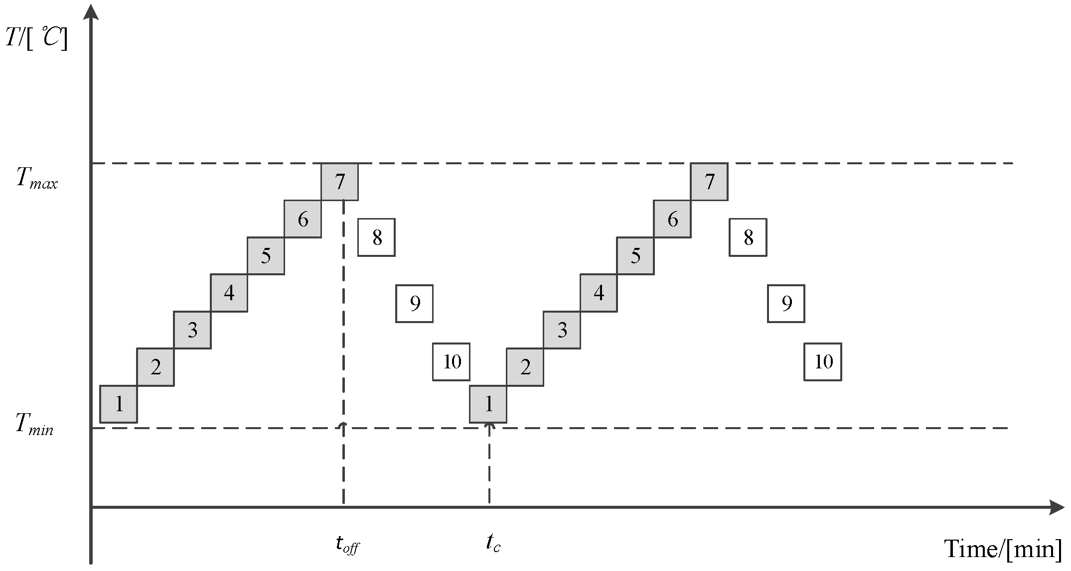
Figure 3.
Initial system load curve.

Figure 4.
Wind power scenarios.

Figure 5.
Ambient temperature curve.
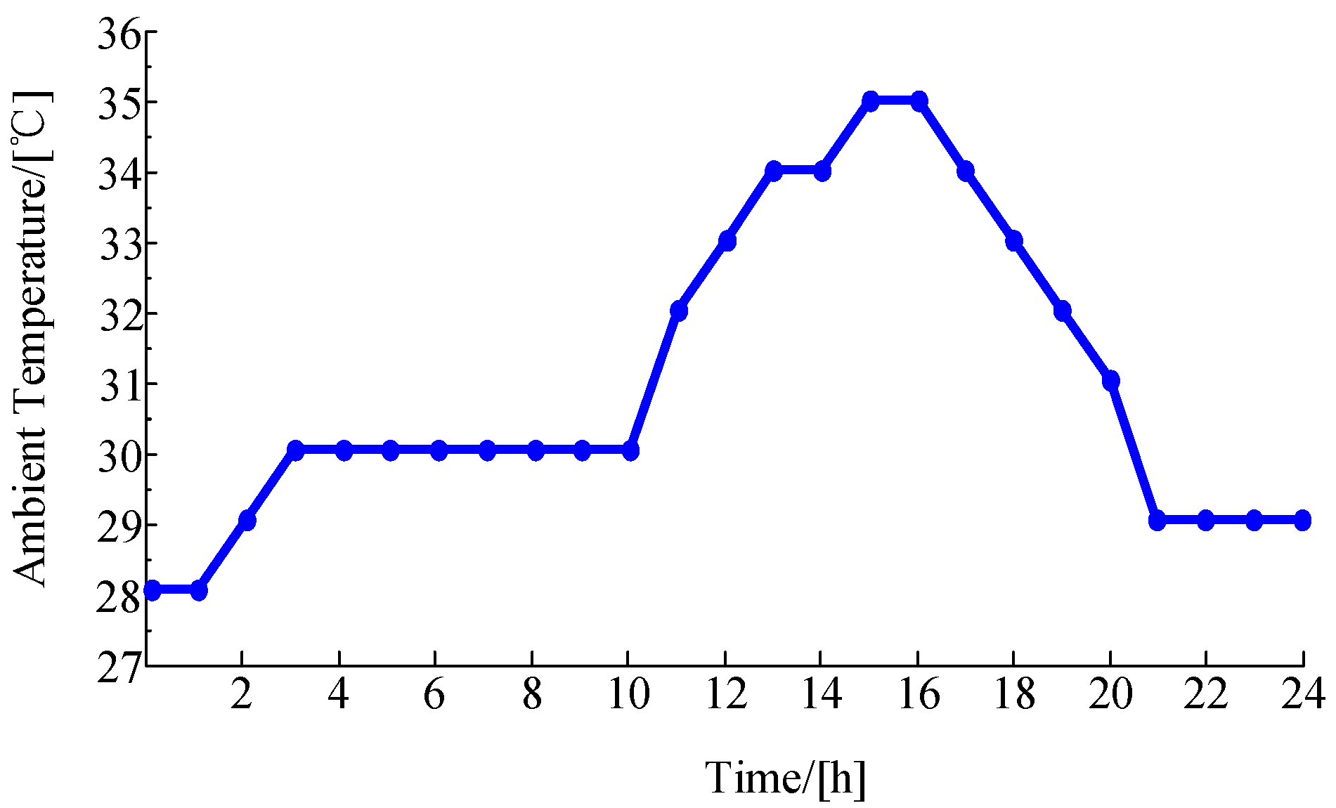
Figure 6.
Load reduction curves in Mode 2.
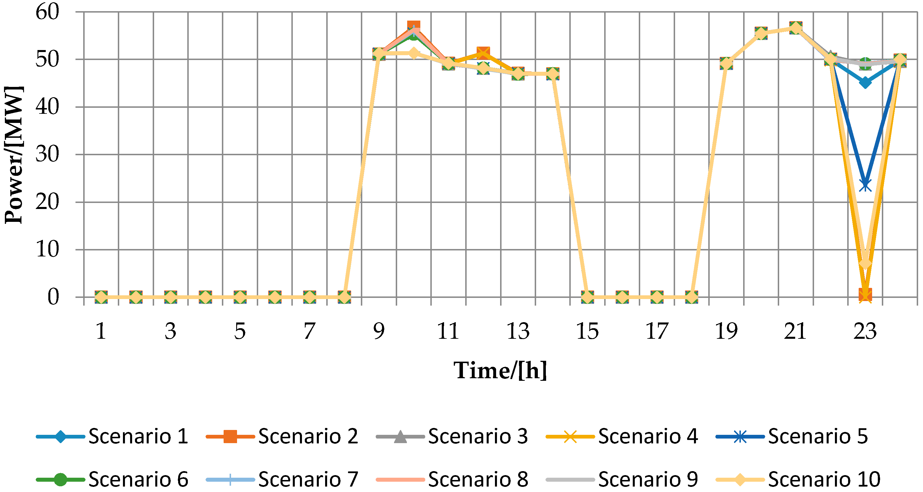
Figure 7.
Load reduction curves under different scenarios (the values of K1 in the first- and second-type air-conditioning load (ACL) are 1 and 0.9, respectively).
Figure 7.
Load reduction curves under different scenarios (the values of K1 in the first- and second-type air-conditioning load (ACL) are 1 and 0.9, respectively).
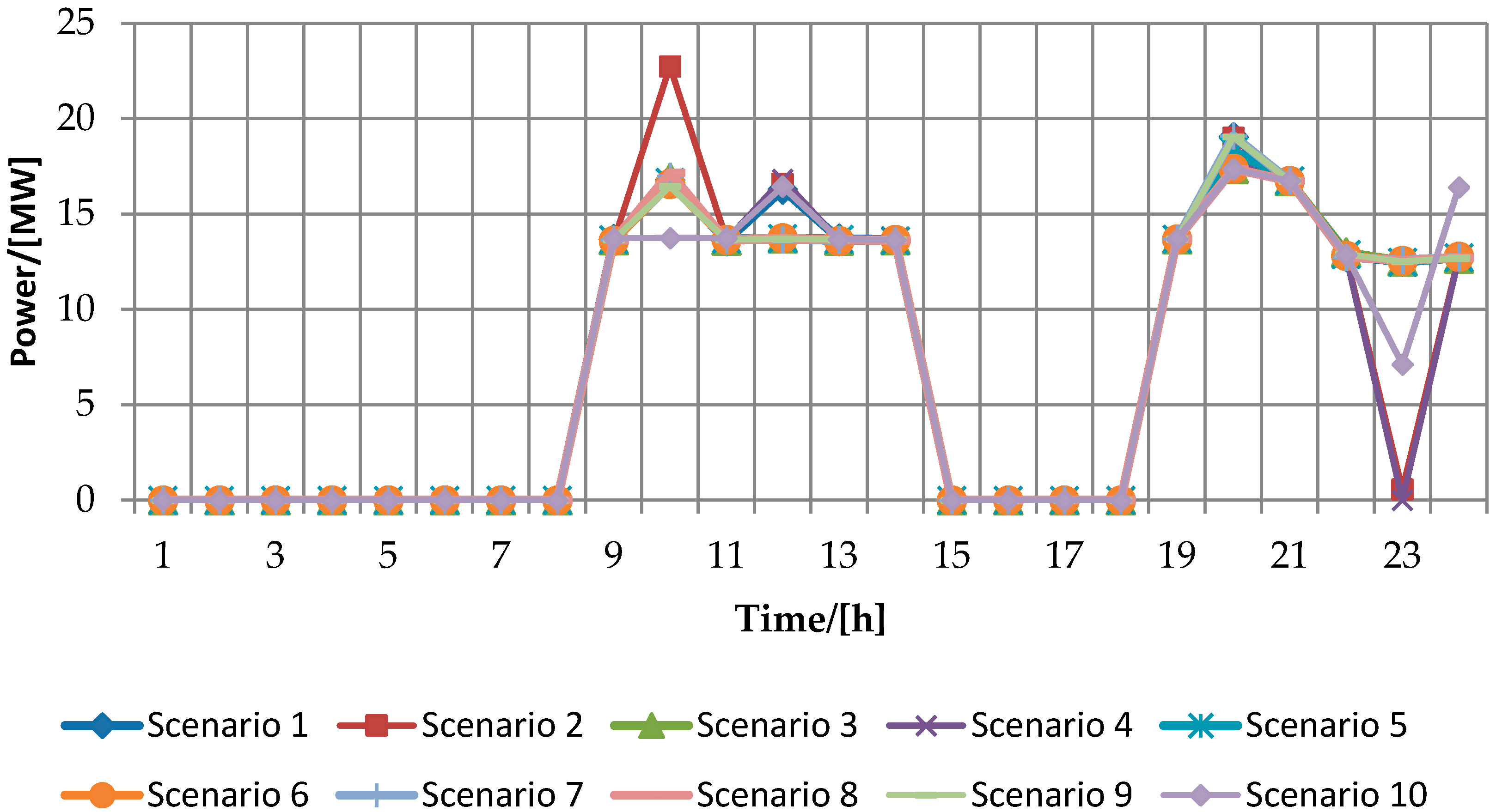
Figure 8.
Load reduction curves under different scenarios (the values of K1 in the first- and second-type air-conditioning load (ACL) are 0.06 and 0.04, respectively).
Figure 8.
Load reduction curves under different scenarios (the values of K1 in the first- and second-type air-conditioning load (ACL) are 0.06 and 0.04, respectively).
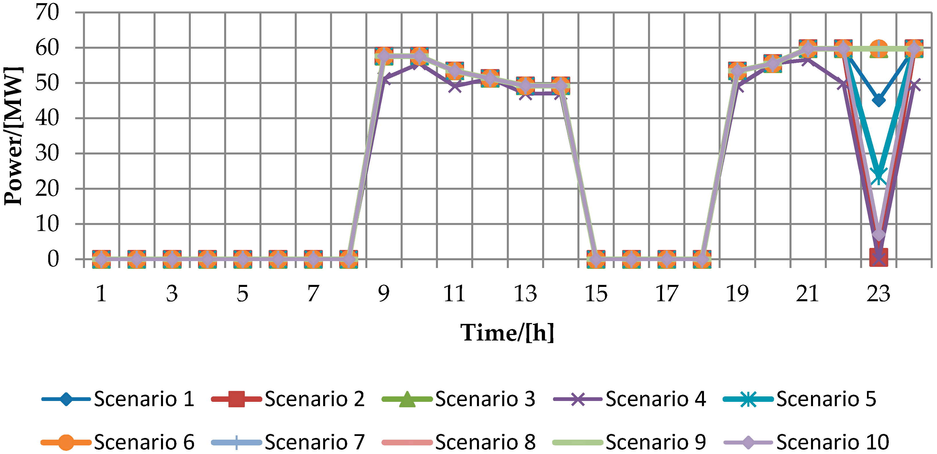
Figure 9.
Load reduction curves under different scenarios (25%).

Table 1.
Parameters of the equivalent thermal parameters model.
| Variable | Value | Variable | Value |
|---|---|---|---|
| Tmin/°C | 22 | e−Δt/RC | 0.96 |
| Tmax/°C | 27 | /kW | 2.5 |
| η | 2.5 | A | 0.18 |
Table 2.
Parameters of the compensation cost.
| ACL Type | K1/$/((MW)2h) | K2/$/(MWh) |
|---|---|---|
| 1 | 0.3 | 4 |
| 2 | 0.2 | 5 |
Table 3.
Comparison of unit commitment results in two modes.
| Mode Type | Unit Commitment (24 h) | ||||||||||||||||||||||||
|---|---|---|---|---|---|---|---|---|---|---|---|---|---|---|---|---|---|---|---|---|---|---|---|---|---|
| Mode 1 | Units | 1 | 2 | 3 | 4 | 5 | 6 | 7 | 8 | 9 | 10 | 11 | 12 | 13 | 14 | 15 | 16 | 17 | 18 | 19 | 20 | 21 | 22 | 23 | 24 |
| 1 | 1 | 1 | 1 | 1 | 1 | 1 | 1 | 1 | 1 | 1 | 1 | 1 | 1 | 1 | 1 | 1 | 1 | 1 | 1 | 1 | 1 | 1 | 1 | 1 | |
| 2 | 1 | 1 | 1 | 1 | 1 | 1 | 1 | 1 | 1 | 1 | 1 | 1 | 1 | 1 | 1 | 1 | 1 | 1 | 1 | 1 | 1 | 1 | 1 | 0 | |
| 3 | 0 | 0 | 0 | 0 | 0 | 0 | 0 | 0 | 0 | 0 | 0 | 0 | 0 | 0 | 0 | 0 | 0 | 1 | 1 | 1 | 1 | 1 | 0 | 0 | |
| 4 | 0 | 0 | 0 | 0 | 0 | 0 | 0 | 0 | 0 | 0 | 0 | 0 | 0 | 0 | 0 | 0 | 0 | 1 | 1 | 1 | 1 | 1 | 1 | 0 | |
| 5 | 0 | 0 | 0 | 0 | 0 | 0 | 0 | 0 | 1 | 1 | 1 | 1 | 1 | 1 | 1 | 1 | 1 | 1 | 1 | 1 | 1 | 1 | 1 | 1 | |
| 6 | 0 | 0 | 0 | 0 | 0 | 0 | 0 | 0 | 0 | 0 | 0 | 1 | 1 | 1 | 0 | 0 | 0 | 0 | 1 | 1 | 1 | 1 | 0 | 0 | |
| 7 | 0 | 0 | 0 | 0 | 0 | 0 | 0 | 0 | 0 | 0 | 0 | 0 | 0 | 0 | 0 | 0 | 0 | 0 | 0 | 0 | 0 | 0 | 0 | 0 | |
| 8 | 0 | 0 | 0 | 0 | 0 | 0 | 0 | 0 | 0 | 0 | 0 | 0 | 0 | 0 | 0 | 0 | 0 | 0 | 0 | 0 | 0 | 0 | 0 | 0 | |
| 9 | 0 | 0 | 0 | 0 | 0 | 0 | 0 | 0 | 0 | 0 | 0 | 0 | 0 | 0 | 0 | 0 | 0 | 0 | 0 | 0 | 0 | 0 | 0 | 0 | |
| 10 | 0 | 0 | 0 | 0 | 0 | 0 | 0 | 0 | 0 | 0 | 0 | 0 | 0 | 0 | 0 | 0 | 0 | 0 | 0 | 0 | 0 | 0 | 0 | 0 | |
| Mode 2 | Units | 1 | 2 | 3 | 4 | 5 | 6 | 7 | 8 | 9 | 10 | 11 | 12 | 13 | 14 | 15 | 16 | 17 | 18 | 19 | 20 | 21 | 22 | 23 | 24 |
| 1 | 1 | 1 | 1 | 1 | 1 | 1 | 1 | 1 | 1 | 1 | 1 | 1 | 1 | 1 | 1 | 1 | 1 | 1 | 1 | 1 | 1 | 1 | 1 | 1 | |
| 2 | 1 | 1 | 1 | 1 | 1 | 1 | 1 | 1 | 1 | 1 | 1 | 1 | 1 | 1 | 1 | 1 | 1 | 1 | 1 | 1 | 1 | 1 | 1 | 0 | |
| 3 | 0 | 0 | 0 | 0 | 0 | 0 | 0 | 0 | 0 | 0 | 0 | 0 | 0 | 0 | 0 | 0 | 0 | 1 | 1 | 1 | 1 | 1 | 0 | 0 | |
| 4 | 0 | 0 | 0 | 0 | 0 | 0 | 0 | 0 | 0 | 0 | 0 | 0 | 0 | 0 | 0 | 0 | 0 | 1 | 1 | 1 | 1 | 1 | 0 | 0 | |
| 5 | 0 | 0 | 0 | 0 | 0 | 0 | 0 | 0 | 1 | 1 | 1 | 1 | 1 | 1 | 1 | 1 | 1 | 1 | 1 | 1 | 1 | 1 | 1 | 1 | |
| 6 | 0 | 0 | 0 | 0 | 0 | 0 | 0 | 0 | 0 | 0 | 0 | 1 | 1 | 1 | 0 | 0 | 0 | 0 | 0 | 0 | 1 | 1 | 0 | 0 | |
| 7 | 0 | 0 | 0 | 0 | 0 | 0 | 0 | 0 | 0 | 0 | 0 | 0 | 0 | 0 | 0 | 0 | 0 | 0 | 0 | 0 | 0 | 0 | 0 | 0 | |
| 8 | 0 | 0 | 0 | 0 | 0 | 0 | 0 | 0 | 0 | 0 | 0 | 0 | 0 | 0 | 0 | 0 | 0 | 0 | 0 | 0 | 0 | 0 | 0 | 0 | |
| 9 | 0 | 0 | 0 | 0 | 0 | 0 | 0 | 0 | 0 | 0 | 0 | 0 | 0 | 0 | 0 | 0 | 0 | 0 | 0 | 0 | 0 | 0 | 0 | 0 | |
| 10 | 0 | 0 | 0 | 0 | 0 | 0 | 0 | 0 | 0 | 0 | 0 | 0 | 0 | 0 | 0 | 0 | 0 | 0 | 0 | 0 | 0 | 0 | 0 | 0 | |
Table 4.
Optimal scheduling cost analysis.
| Cost/($) | Mode 1 | Mode 2 |
|---|---|---|
| Power generation cost | 419,422.71 | 401,847.44 |
| Cost of start-up | 2920 | 2638 |
| Cost of ACL reduction | 0 | 6348.7 |
| Total cost of objective function | 422,342.71 | 410,834.14 |
© 2017 by the authors. Licensee MDPI, Basel, Switzerland. This article is an open access article distributed under the terms and conditions of the Creative Commons Attribution (CC BY) license (http://creativecommons.org/licenses/by/4.0/).
Share and Cite
MDPI and ACS Style
Han, X.; Zhou, M.; Li, G.; Lee, K.Y. Stochastic Unit Commitment of Wind-Integrated Power System Considering Air-Conditioning Loads for Demand Response. Appl. Sci. 2017, 7, 1154. https://doi.org/10.3390/app7111154
AMA Style
Han X, Zhou M, Li G, Lee KY. Stochastic Unit Commitment of Wind-Integrated Power System Considering Air-Conditioning Loads for Demand Response. Applied Sciences. 2017; 7(11):1154. https://doi.org/10.3390/app7111154
Chicago/Turabian StyleHan, Xiao, Ming Zhou, Gengyin Li, and Kwang Y. Lee. 2017. "Stochastic Unit Commitment of Wind-Integrated Power System Considering Air-Conditioning Loads for Demand Response" Applied Sciences 7, no. 11: 1154. https://doi.org/10.3390/app7111154
Note that from the first issue of 2016, this journal uses article numbers instead of page numbers. See further details here.