Machine Learning for Identifying Demand Patterns of Home Energy Management Systems with Dynamic Electricity Pricing

1
Department of Technology and Operations Management, Rotterdam School of Management, Erasmus University, Burgemeester Oudlaan 50, 3062PA Rotterdam, The Netherlands
2
Google Ireland Ltd, Google Docks, Barrow Street, D04 V4X7 Dublin, Ireland
3
Faculty of Management, Economics and Social Sciences, University of Cologne, Universitaetsstrasse 24, 50931 Cologne, Germany
4
Institute of Energy Economics, University of Cologne; Vogelsanger Str. 321a, 50827 Cologne, Germany
*
Author to whom correspondence should be addressed.
Appl. Sci. 2017, 7(11), 1160; https://doi.org/10.3390/app7111160
Submission received: 16 October 2017
/
Revised: 4 November 2017
/
Accepted: 6 November 2017
/
Published: 12 November 2017
(This article belongs to the Special Issue Smart Home and Energy Management Systems)
Abstract
:Energy management plays a crucial role in providing necessary system flexibility to deal with the ongoing integration of volatile and intermittent energy sources. Demand Response (DR) programs enhance demand flexibility by communicating energy market price volatility to the end-consumer. In such environments, home energy management systems assist the use of flexible end-appliances, based upon the individual consumer’s personal preferences and beliefs. However, with the latter heterogeneously distributed, not all dynamic pricing schemes are equally adequate for the individual needs of households. We conduct one of the first large scale natural experiments, with multiple dynamic pricing schemes for end consumers, allowing us to analyze different demand behavior in relation with household attributes. We apply a spectral relaxation clustering approach to show distinct groups of households within the two most used dynamic pricing schemes: Time-Of-Use and Real-Time Pricing. The results indicate that a more effective design of smart home energy management systems can lead to a better fit between customer and electricity tariff in order to reduce costs, enhance predictability and stability of load and allow for more optimal use of demand flexibility by such systems.
1. Introduction
The energy business is going through a series of swift and radical transformations to meet the growing demands for sustainable energy. The future of the energy sector will, to a large extent, be formed by a transformation in the electricity sector, posing challenges for traditional electrical power systems. This shift is of a complex nature, but offers ample opportunities for business and information analytics to support the transition [1]. The electricity grid faces decentralized production from renewable sources, electric mobility, and related advances. These are at odds with traditional power systems, where central large-scale generation of electricity follows inelastic consumer demand. Additionally, renewable electricity sources are, unlike traditional sources, volatile in nature and strongly dependent on external factors such as weather conditions, making short-term energy production forecasting increasingly important [2]. The non-storability and volatile aspect of sustainable energy sources and the required shift from a demand-driven to a supply-driven market means the energy transition requires system flexibility from all market participants.
On the retail side, end-consumers can offer demand flexibility to the grid by shifting their load on moments of peak demand to other times in the day. Energy services and utilities can incentivize such behavior [3], by optimizing feedback to their customers and enabling new forms of dynamic trading. Energy Management Systems (EMS) can control the use of end-appliances and optimize the flexible range, based upon the end consumer’s personal preferences and beliefs [4]. Demand Response (DR) programs offer financial incentives to take action to reduce or shift load in correspondence to market price behavior. As such, DR builds upon the behavioral traits of energy consumers via comprehensive communication through home energy systems. The effectiveness of such programs is largely affected by the willingness of end-users to be involved in such programs [5]. Engaging customers requires systematic communication and interaction between the utility provider and the people it serves, with the intent of building trust, respect, and achieving optimal energy usage amongst the heterogeneity of individual households.
The heterogeneity amongst customers ensures that EMS and the energy service provider have to learn from the customer’s individual preferences in order to make optimal recommendations in terms of dynamic tariff targeting, and ultimately, consumer welfare. We apply machine learning techniques in this paper, to show how such systems can recommend tariff schemes based upon the individual household’s attributes. Our setting is a natural experiment, involving real-world customers of a national utility company participating via dynamic pricing contracts. This allows us to reach high ecological validity in testing, whether the increase of household informedness influences demand for individual households, and how utilities can use machine learning techniques in designing their home energy management systems for better targeting of customers.
With utility providers starting to introduce dynamic price tariff schemes to residential households, demand side flexibility may enhance stabilizing the grid load under the right price incentives [6]. Demand side management strategies, such as demand response, can have a dual effect of reducing electricity consumption and allowing greater efficiency and flexibility in grid management [7]. Demand response refers to a wide range of actions that can be taken on the customer side of the electricity meter, in order to respond to specific conditions within the electricity system [8]. The different DR programs can generally be classified into two main categories, namely Incentive-Based Programs (IBP) and Price-based Programs (PBP) [9]. In PBP programs, consumers are offered dynamic pricing rates over time, typically with prices significantly higher during peak-periods than during off-peak periods.
In this study, we focus on the two most widely used programs within PBP. The tariffs offered to end customers in the set-up of our natural experiment are Time-Of-Use (TOU) and Real-Time Pricing (RTP) pricing. Both tariff schemes vary according to timing and impact on process quality [10]. TOU pricing is changing the unit price of electricity during specific time periods at a fixed rate. The tariff tries to encourage customers to shift the consumption from peak to off-peak periods, by reflecting the production and investment cost structure with higher rates during high demand periods. The tariff variations are, however, predetermined and fixed at delivery, making it easily interpretable for the customer to optimize his portfolio. Market DR (Demand Response) relies on Real-Time Pricing (RTP) or wholesale market spot prices, where price signals reflect supply conditions. Although this creates a higher level of demand flexibility for the system, it requires a higher involvement from a customer perspective. Therefore, as customer involvement is dependent on the tariff scheme, correct customer targeting can enhance utility portfolio optimization and by extension smart grid management. In RTP schemes, customers are informed about, mostly hourly changing, varying electricity prices on a day-ahead or hour-ahead basis [11]. Given the recent technological developments and an advanced metering infrastructure worldwide, effective communication of prices and detailed load profiles between utility providers and electricity consumers have become possible. Dynamic pricing schemes are usually based on retail prices and reflect real-time system costs, thus encouraging energy consumers to reduce or shift energy consumption during high wholesale price periods.
This study contributes to the growing stream of literature discussing the effects of electricity prices on energy consumption behavior. It is argued that the effectiveness of energy information is not generalizable across cultures and demographic groups [12] and large variations in effect sizes and significance of different electricity pricing types can be found. Previous studies suggest that dynamic pricing strategies would encourage the price-responsive demand to balance supply and demand of electricity [13], with various dynamic pricing schemes impacting consumption behavior of residential households in different ways [14]. The first ever hourly Real-Time Pricing (RTP) program for residential customers, however, was only conducted in 2011 in Chicago. The results of the demand estimates of the respective study suggest that dynamic prices only influence the residential electricity demand during peak hours. More specifically, it shows that participating residential households were engaged in peak shaving behavior, but not in load shifting behavior [15]. Earlier work however suggests different results depending on the dynamic pricing scheme, where demand based TOU electricity tariffs have decreased peak demand and shifted electricity demand from peak to off-peak periods [16]. We contribute by analyzing both respective dynamic pricing schemes, comparing TOU pricing performance to Real-Time Pricing schemes in the same natural experiment. Our study extends the current line of literature by providing results from one of the first natural large-scale open sign up experiments involving dynamic electricity prices. In addition, we focus on the individual preferences and beliefs of each individual, crucial for learning of smart home energy management systems, as household attributes influence price sensitivity and the effectiveness of the dynamic pricing schemes [17].
Household attributes have been proven to play an important role in explaining how willing energy users are to conserve energy [18]. Di Cosmo et al. [19] have found evidence that the influence of electricity prices is different across household groups. Households with higher income, higher education levels, and higher electricity use are more reactive to energy consumption behavior change than other groups [20,21]. In contrast, other feedback studies could not find a clear link between household-level characteristics and price effectiveness [22]. In addition to the influence of electricity prices on absolute electricity consumption, the effect of building characteristics and socio-demographic information significantly influence energy demand behavior. Testing TOU demand behavior in Germany, Schleich and Klobasa [23] find that the size of a household’s building positively influences energy consumption and that the number of appliances positively influences the electricity consumption. The number of occupants of a household, the building size of a household, the building type, and the number of bedrooms is found to positively influence electricity consumption [24]. A study characterizing domestic electricity consumption patterns in Ireland found that the number of occupants, the building size and the building type positively influence residential electricity consumption [25]. Contradictory findings have been reported as well, for example the authors of [26] investigate determinants of residential electricity consumption, finding that the number of occupants and the building size are positively associated with electricity consumption, while the building type and the building age are not associated with electricity consumption. A study investigating short- and long-term price elasticity [27] found that income positively influences peak and off-peak residential electricity consumption, while the household size does not show any significant influence. Whereas the previously mentioned studies investigate the influence of household attributes in a flat or TOU pricing environment, little work has been done in dynamic RTP settings, let alone comparing tariff schemes. Alberini, Gans and Velez-Lopez [28] find that in a dynamic tariff scheme, only building type shows a significant influence on electricity usage, but they do not compare the variety of household attributes to other tariff schemes. Our study is one of the first to analyze for both TOU and RTP, and validate the efficient targeting for utility companies in terms of these characteristics. An overview of related literature can be found in Table 1.
With the growth of home energy management systems and smart meters, the volume, frequency and variety of information is growing exponentially [29]. Business intelligence and machine learning techniques can provide utilities and energy-market-related companies with demand forecasts and customer usage patterns to support data-driven decision making. In such a high-dimension space with high frequent multi-variable data as the above context, developing effective clustering methods for customer patterns is a challenging problem, due to the curse of dimensionality [30]. We apply spectral relaxation by a Principal Component Analysis (PCA) to find a meaningful representation of the intrinsic dimensionality of the data and perform a k-means clustering analysis in the projected space, to analyze distinct customer group behavior from the natural experiment. This method has become one of the important machine learning algorithms for learning consumer behavior [31], particularly for energy demand forecasting [32,33]. Our paper makes several contributions to both dynamic pricing literature and the design of home energy management systems. First, the study shows that time capabilities play a significant role when examining usage behavior in dynamic price settings. By looking at each hour independently, we aim to identify specific times during the day, in which the households are adapting their behavior more rigorously in order to take advantage of varying price levels. We confirm different daily demand profiles for both tariff schemes and find evidence for a significant influence of household attributes. These attributes influence our different household clusters, which have varying capabilities to react to the respective dynamic pricing scheme. Implementing machine learning algorithms in EMS for identified households by utility companies, should lead to better fit between customer and electricity tariff in order to reduce costs, enhance predictability and stability of load and allow for more optimal use of demand flexibility by the EMS.
The rest of this paper is organized as follows. Section 2 clarifies the design and set-up of our natural experiment. Section 3.1 describes the effects of dynamic pricing schemes on energy demand in relation with household attributes. Section 3.2 describes the proposed clustering algorithm and discusses the distinct groups for targeting home energy management purposes. Finally, Section 4 discusses the findings and draws conclusions with future scope.
2. Design of Natural Experiment
A natural experiment in which real-world end-users are exposed to dynamic pricing schemes is set in order to identify demand patterns of residential households. The experiment is designed in collaboration with a Dutch utility company. The study was carried out in collaboration with Qurrent Energie, providing access to the natural experiment. Although similar case studies have been carried out before [34], the dynamic pricing scheme roll-out was the first to combine different dynamic pricing schemes on a large-scale sign-up basis, providing flat and different dynamic tariff options nationwide since late 2016. Households were proactively approached and asked for voluntary participation. The allocation of the usage of the customers is done on the basis of smart meter (P4) data, with a central server communicating tariffs and reading data to individual households and their energy management systems. An overview of the origin of information and data signals can be found in Figure 1.
Large-scale generators sell the produced electricity on wholesale markets to retailers or utility companies. The merit order curve of wholesale electricity markets varies depending on market fundamentals of the underlying fuels, such as the oil and gas price, and variability of weather conditions for renewable power plants. Wholesale price formation depends on the generation costs of the marginal technology in competitive power wholesale markets and elasticity of retailer demand. Where renewables run at low marginal cost, mainly consisting out of maintenance costs, coal fired power plants and several types of gas power plants run at higher marginal costs, typically due to fuel costs, however have a higher degree of flexibility [35].
Utility companies engage in financial contracts with their customers on retail markets. The tariff scheme for the customer is set by the utility company, determining for every contract the time-granularity of the information stream between wholesale markets and retail markets. Depending on the contract, home energy management systems can guide the customer or act upon his preferences and beliefs in order to optimize his demand profile, where monetary incentives are given by dynamic tariff schemes. With end-appliances becoming highly digitized, so-called prosumers can consume and locally generate production. Distributed production and demand add more flexibility within smart grids and opportunities arise for end-users to shift electricity demand throughout the day. It is therefore of importance for the utility company to offer correct price signals to its customers and optimally target them according individual preferences. As these may vary according to the heterogeneity amongst customers depending on household attributes, we aim to identify behaviors of customers operating a home energy management system in dynamic price settings.
The digitization process of the electricity sector in recent decades has created new services, products and markets, in addition to reshaping existing technical systems and infrastructure. New mechanisms are put in place with data generated by numerous smart devices connected in a so-called network Internet of Things, and opportunities arise in the context of energy and electricity markets [3]. The digitalization of energy services can improve utility providers’ understanding of increasingly uncertain energy production and consumption, while encouraging a better way of communication with electricity consumers and providing electricity consumers with new information about their use of electricity. Smart grids paired with smart meters provide both supply and demand valuable real-time information on energy flows and consumption, giving also consumers more control over their energy usage, and enabling the development and expansion of demand-side management programs, contributing to needed flexibility in volatile energy systems. In such fast-evolving domains as smart energy markets, it is necessary to develop and adapt existing pricing methods within changing market dynamics, taking into account individual user preferences and objectives with respect to the decision context.
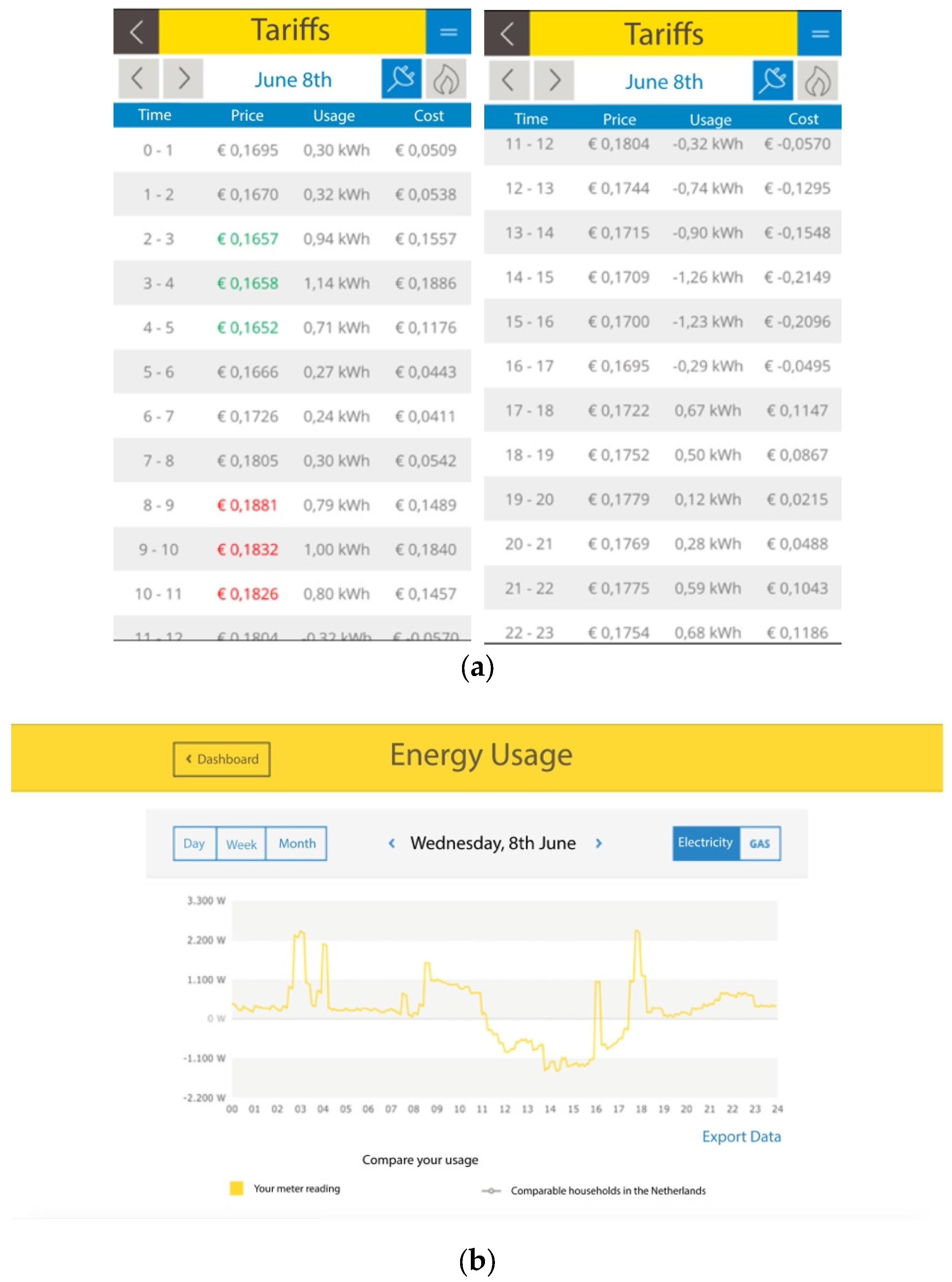
The Real-Time Prices offered in the experiment are electricity retail prices based upon the Dutch spot wholesale electricity market, APX [36] and are forwarded to the participating households on a day-ahead basis. The TOU prices vary between a peak period and an off-peak period, depending on the month-ahead forward price for electricity and a risk premium according peak and off-peak. Both tariffs are supplemented with a fixed number for surcharges, namely balancing, sustainability guarantees and energy taxes. Prior to the start of the experiment, electricity home energy management devices are installed in all households. As such, households gained access to real-time energy consumption and electricity prices through a web-based dashboard for Notebooks, Smartphones and Tablets. This home energy management system thus allows customers to get a better, real-time understanding of their energy-related activities. A tariff overview allows for the proper review of past household electricity usage behavior, electricity prices and final cost of electricity usage throughout the day. The web application displays usage to the users as the net electricity consumption of a household. Negative usage values indicate that the user generates more electricity than consumed. The respective negative values in the cost column indicate the discount granted to the household for the next electricity bill. A visualization of the web application can be found in Figure 2.
The home energy management system allows households to get a better overview of past usage behavior and future outlook in the form of next day prices by a dashboard visualizing consumption and production next to general functions, such as profile, metering, messages and a financial overview. The users can examine the respective load profiles for electricity and gas for any given point in the past on daily, weekly or monthly levels. Additionally, users can compare their load profile with the load profile of comparable households in the Netherlands. The households have the option of exporting their usage data from the dashboard for a more in-depth analysis. The hourly electricity tariffs are communicated on a day-ahead basis via the home energy management system.
At the beginning of the experimental period, the RTP group receives the hourly real-time electricity prices of the following day, while the TOU group continues to receive the standard time-of-use electricity prices of the energy provider. We selected data from households post experiment, when no privacy concerns were indicated by the individual households. In total, our dataset consists of 78 households in the RTP group, and 150 households for the TOU group. Both groups had access to the home energy management system of the energy provider, and were able to observe their energy consumption in real-time. Next to measuring the energy demand, the selected households answered a survey post experiment about specific attributes and characteristics of their households. Specifically, the survey asked the households about the number of occupants, the type of house, the insulation of the house, the location, the size, the type of heating, and the use of solar panels. An extensive descriptive overview of nomenclature and all measured variables can be found in Appendix A.
Table 2 presents the descriptive statistics of our sample. The average number of household occupants is 2.63 for the RTP group and 2.97 in the TOU group. The average building age of the sample, average building size, building type, heating type and roof insulation experienced similar levels for control and treatment group. No significant differences in terms of our main variables could be found; however, in order to account for the fact that there may be unobserved differences between our households, we have used household fixed effects in our analysis.
3. Results
3.1. Panel Data Analysis of Dynamic Pricing Schemes
We analyze how the RTP and TOU treatment perform in terms of demand variation, in order to validate both schemes and their difference in behavior. Assuming that each household has his very own price sensitivity and energy usage patterns, a panel data regression is capable of assessing the statistical significance of the individual variables within each separate panel. It also accounts for individual-level heterogeneity, making it possible to control for variables that are not measurable, per se, across households or across time. We apply a panel data regression to measure the behavior of entities as households across time [37], allowing double-subscripts on the variables, taking cross-sections into account as well as time-dimensions. We denote:
where the is the dependent variable, representing a form of the demand of household i during the hour t of the day, with error . In order to study how the behavior depending on treatment throughout the day, we take an hourly approach. Coefficient reflects household-fixed effects that record potential time-invariant, household-level heterogeneity related to the net electricity usage. represents the vector of coefficient estimates of dimension N of explanatory variables . More information on the explanatory variables can be found in Appendix Table A2.
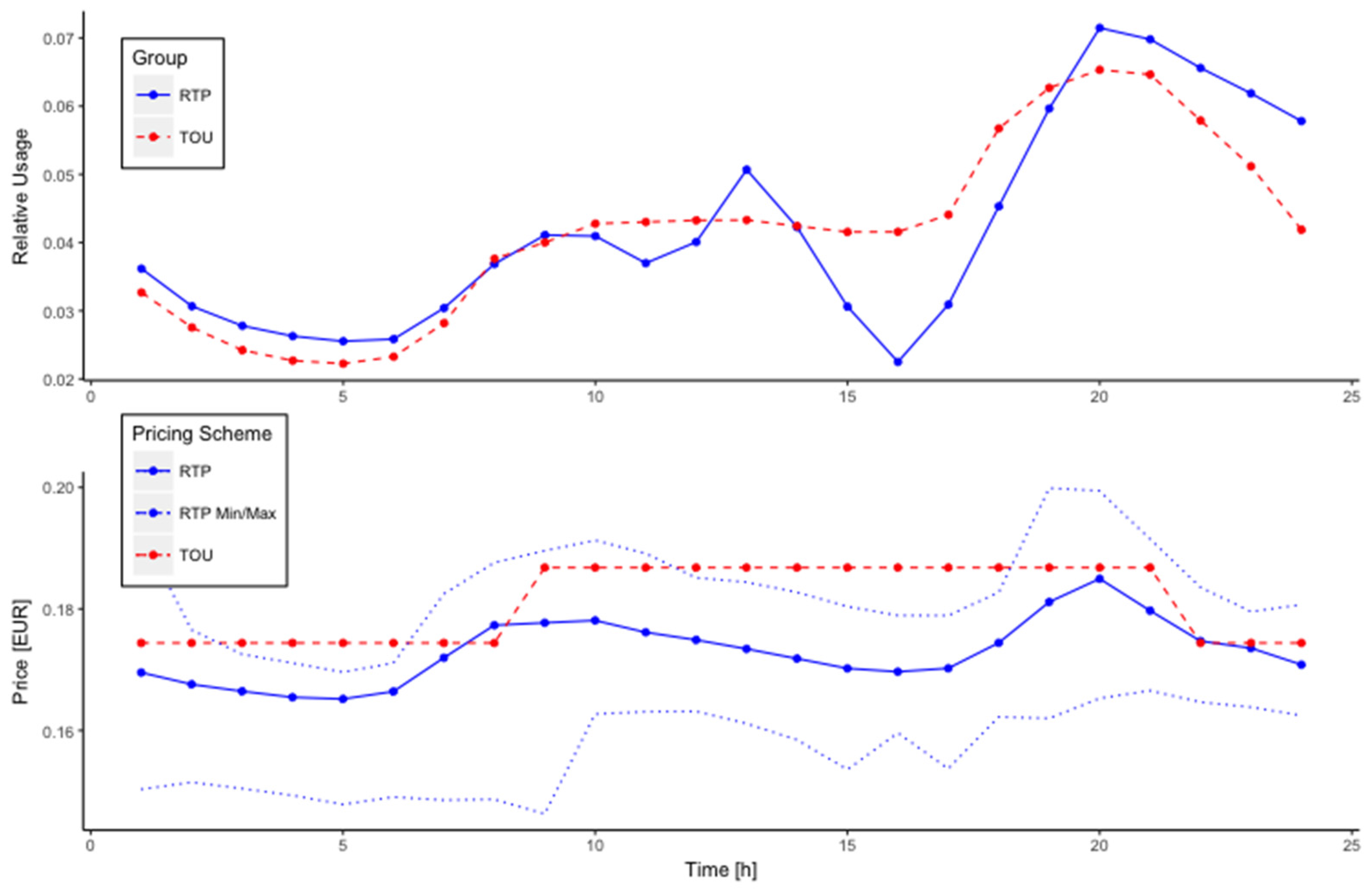
We verify different behavior between the tariff schemes in two steps. First, we verify demand shifting behavior for both treatments analyzing relative electricity usage throughout the day. We set the dependent variable in (1) to electricity usage relative to total daily usage , comparing daily usage across treatments. The updated coefficient estimate is two-dimensional, consisting of the main effect for price and control effect for solar influx. Figure 3 visualizes the relative electricity usage and the average daily electricity price for both tariff schemes. Load shifting behavior occurs more dominantly in the RTP treatment as expected, occurring between 3 p.m. and 9 p.m., corresponding to higher prices for electricity usage. This is compensated for by relatively higher demand from late evening until late morning.
Table 3 gives the differences in regression coefficients between the control and treatment groups. The results show that both dynamic electricity price schemes have a positive significant relationship with relative electricity usage. When we control for interaction effects in the single model, we find a significant negative difference in slopes for the price variable for both treatments (). We thus find that the price difference effect is smaller for RTP treatment than it is for the TOU treatment. Although counterintuitive at first, we argue that this comes from the fact that RTP behavior is less reactive to price differences around peak times, as indicated by Figure 3, finding evidence for differing load shifting behavior between both dynamic price settings.
Next, we analyze what effect household attributes have on demand patterns throughout the day. We verify whether these effects are significantly tariff dependent by regressing on the willingness to use energy, and set the dependent variable in (1) to price sensitivity . We test for multicollinearity by observing correlations between household variables, but find that the predictor variables correlate enough to bias results. We perform a Hausman test, to select random effects or fixed effects for the panel data regression [38]. This approach ensures the sufficient measurement of the interrelatedness of the variables of this study, while accounting for individual differences across households and time. Controlling for fixed effects obliges us to explore the relationship between the proposed individual and outcome variables within a household. A random effect model assumes that entity error terms are not correlated with the household level attributes. As the Hausman test was insignificant for all 24 data sets, we make use of random effects. Results can be found in Table A3 and Table A4 in Appendix B and Appendix C.
When examining the 24 different panel data regression coefficients between the RTP and TOU treatment groups, it becomes evident that the household attributes have a very different influence on both groups. The observed differences are either time-differentiated or show an opposite relationship with the willingness to use electrical energy. We find that some variables, such as the building size, have a distinct time gap in which the influence of the variable is not relevant. Moreover, the variables of building type and roof insulation are shown to be insignificant in the overall panel data regression, but have specific times during the day in which they indeed are significant.
Lastly, we test for significant differences between treatment coefficients. We introduce RTP as a dummy variable for the Real-Time Price treatment, and connect it with all the coefficients of interest. As the above regression indicated error terms to be independent for both treatments, we form the combined model. With representing the difference in slope between both coefficients, allowing for testing the difference in slopes between regression coefficients. Results are given in Table 4.
We find that the willingness to use electricity is negatively correlated with building age, building size and building type. The analysis indicates that households in the RTP group have a significantly lower willingness to use electricity according to the mentioned household attributes. However, we find a significant positive correlation for the number of household occupants. We argue that this may be the case for larger families, where the utility of shifting demand is lower due to a more inelastic demand curve.
The panel regression analysis shows a clear influence of household attributes on the effect of energy demand by home energy systems operating under dynamic pricing contracts. Home energy management systems with different tariff structures lead to different types of behavior from the customer, depending on their household attributes. Home energy management systems should learn from their customers, via a smart home device or intelligent agent, recommending optimal tariffs to both customer and utility, based upon the individual’s preferences and beliefs. The next section makes use of machine learning techniques to achieve this goal.
3.2. Reduced Dimension Clustering to Identify Demand Patterns
The development of sensor technologies and network communication technologies, via smart home energy management systems, for example, have had an explosive impact on customer behavior data accumulation. Extracting useful information from the resulting high-frequent multivariate data, machine learning have enormous potential for efficient targeting and steering end-customer behavior [29]. Earlier work has applied various machine learning techniques for customer load curve typification, which can be divided into 5 method groups; partitioning, hierarchical, density-based, grid-based and model-based [39]. Although no single clustering method is always superior to the other, as they are used for specific applications, most commonly used are partitioning models such as k-means, fuzzy c-means clustering and hierarchical. Non-hierarchical clustering methods [40,41] are preferred over hierarchical in order to prioritize the minimization of internal cluster variance and cluster similarity. Fuzzy c-means and probability neural networks have proven to be useful methods for identifying load customer patterns [42]; however for distinct cluster identification, k-means is often preferred for achieving efficient and scalable results [43]. Lastly, in the above context of increasingly large datasets, efficiency can be improved by combining machine learning methods via hybrid approaches [44].
We conduct such a hybrid approach, via a form of spectral relaxation clustering [45], with a kernel Principal Component Analysis (kPCA) combined with k-means, in order to find distinct groups of households for demand targeting by home energy management systems. This section gives a descriptive overview of the reasoning, for a more comprehensive description we refer to earlier work [46]. The analysis shows how applying machine learning techniques should ideally play a role in smart home EMS in order to target individual customers along the individual attributes and send tariff recommendations to the utility.
Spectral relaxation clustering finds the eigenvectors of the data set, which are orthogonal, and aims at explaining the variability of the data in lower dimensionality. The first step involves building a similarity matrix and computing the first k eigenvectors. We apply kernel PCA to ensure an interior solution, in that this method renders the eigenvectors of the covariance matrix. As the principal components are the continuous solution of the cluster membership, the analysis allows for identifying groups in terms of their components, while the groups can be used in terms of regression clustering for optimal targeting purposes. In a second step the algorithm builds a new data matrix, where the column represents the eigenvectors. We interpret the rows of this matrix as our new data points and apply k-means clustering.
The principal component analysis is conducted to identify the most powerful variables for the cluster analysis of our households. The analysis aims to find a set of new variables in order to extract the most important information from the data set and analyze the structure of the observations and variables. The results can be seen in Table 5. The analysis gives the following variables as most important factors for clustering households; number of household occupants, building size, building type and terrain type.
We evaluate the appropriate cluster solution, by examining the absolute differences between the original and random sum of squared errors (SSE) against the chosen cluster solutions. The appropriate cluster solution is given by the solution where the actual SSE differs the most from the mean of the random SSE. This process is shown in Figure 4, giving evidence for selecting 5 as the appropriate number of clusters. We thus proceed with the five strongest variables, of which the first two components explain more than 80% of the point variability of the entire data set.
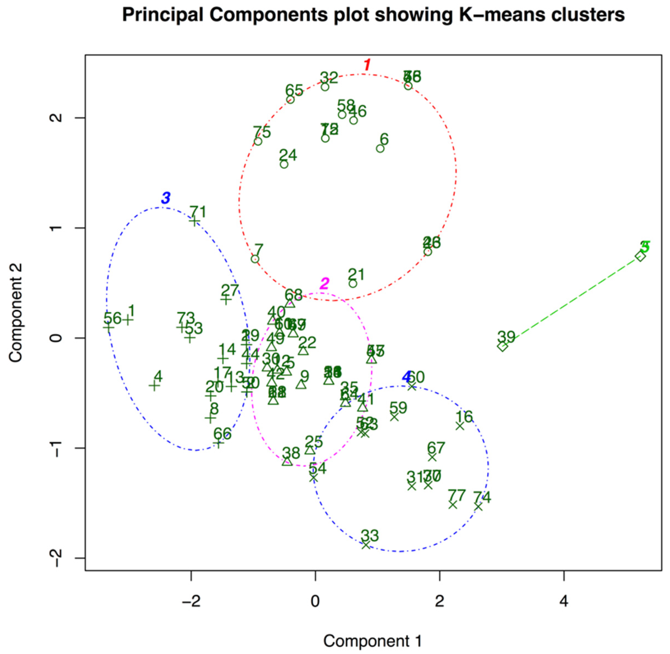
The visualization of the k-means clustering is given in Figure 5 against the two strongest principal components, segmenting the data set into clearly distinguishable clusters. The k-means clustering analysis resulted in a cluster sum-of-squares of 84.31. The two strongest principal components explain 78.17% of the point variability within our sample. Each of the five identified clusters of this study should be seen as an archetype that categorizes the households across our sample, with the respective individual within-cluster variance given within brackets:
- ‘Cluster 1’ (18.09) represents 17% of the participating households. The group of households consists of large groups of people, that are only residing in urban or suburban areas. The majority of this group resides in semi-detached and row-houses. The group represents higher-end urban workers with families.
- ‘Cluster 2’ (15.75) represents the largest group of households with 36%. This group represents households living in urban areas, in row or semi-detached houses. The group represents lower-end urban workers.
- ‘Cluster 3’ (14.07) represents 21% of the participating households. The cluster primarily contains three-person households, which live mostly in detached houses, in the city or rural areas. We identify young starters to be present in this group.
- ‘Cluster 4’ (4.59) is characterized by a small group composition of 2 persons on average. They are represented in all classes of building type and terrain, but with a relatively large size of building. We find this group to consist of mainly seniors.
- ‘Cluster 5’ (31.81) is only comprised of 2 households, relatively small in number of occupants, living in detached houses. As the cluster is not found to be significant, it will be ignored for the following elaborations.
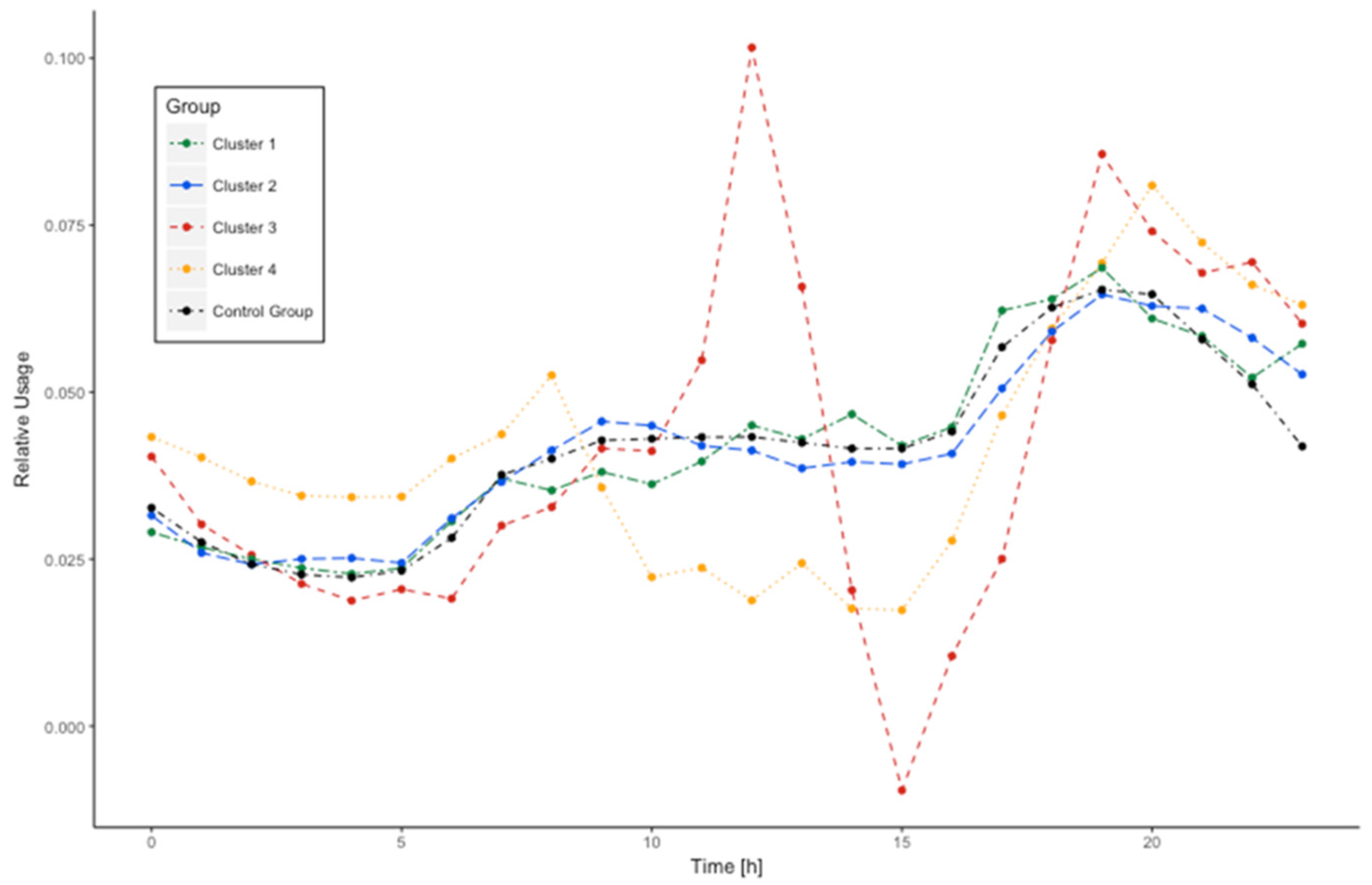
The relative electricity usage across clusters and TOU (control) group is visualized in Figure 6. Cluster 3 is showing extreme behavioral deviations in their relative electricity usage. Comparing it to the relative electricity usage of our control group, it becomes evident that Cluster 3 exchanges part of its daily energy consumption to early noon hours, and saves high amounts during afternoon hours, when the electricity prices are starting to rise again. In addition, Cluster 4 is shows a similarly favorable relative load profile for the Real-Time Prices. More specific, Cluster 4 has an above average relative electricity usage during early morning and late evening times, which are usually the times in which the prices are comparably low. Lastly, Cluster 1 and 2 have very similar relative load profiles compared to the control group.
The results indicate how spectral clustering can help in identifying distinct groups of residential household behavior in relation to their smart home energy management systems. Depending on certain household attributes, we find that specific households are more energy aware and a smart energy management system can beneficially operate the household’s appliances according to market developments. Other households are not as price sensitive, rendering a suboptimal situation when RTP is applied. In this case, energy management systems should recommend a TOU or fixed tariff in order to prevent high peak prices. The analysis indicates the potential of smart home energy management systems, with transparent communication between both parties essential in order to optimally engage residential load in dynamic pricing schemes.
4. Conclusions
Home energy management systems are believed to play a crucial role in efficiently capturing the benefits of DR programs to ensure demand flexibility and peak load reduction. The effectiveness of such programs are, however, largely affected by the willingness of end-users to be involved in such programs. Based upon the individual preferences and beliefs of the customer, not every dynamic pricing program will be as effective for the overall welfare of customer and utility company. This paper, therefore, aims to identify demand patterns of households with the two most-widely used dynamic pricing settings, TOU and RTP pricing. As such, it allows to study a better fit between customer and electricity tariff, allowing for a more optimal use of demand flexibility by the energy management system. Our setting is a natural experiment, involving real-world customers of a national utility company participating via dynamic pricing contracts.
In a first step, we find a significant impact of the dynamic pricing scheme on the relative electricity usage of the individual households and find evidence for different demand behavior based upon the individual household attributes. This indicates the need for individual customer tariff targeting, as static building characteristics, such as building age, building size and building type, and demographic characteristics, such as the number of household occupants, make end-consumers act significantly different in the two dynamic pricing schemes. Secondly, we identify distinct groups of customer demand patterns by conducting a spectral clustering analysis. Our results show clusters with clearly distinguishable behavioral electricity usage patterns. Using machine learning in non-convex data-sets such as household electricity demand data, will allow energy management systems to more optimally target customers based upon individual preferences.
The study presents several conclusions and implications for exploiting smart home energy management systems. By segmenting households based on their household attributes, we are able to isolate groups that differ in their level of engagement with the respective dynamic pricing scheme. This indicates that home energy management systems do not perform equally over a varying set of households, with respect to reducing and shifting load. Our study provides an initial better understanding of households their willingness to engage with dynamic pricing schemes, indicating that successful implementation of home energy management systems will not only be based upon the respective DR program, but also on the individual household preferences and beliefs.
Acknowledgment
Special thanks go to Mark van Loon, Business Development Manager at the Dutch utility company Qurrent Energie, for his guidance and assistance in the experiment.
Author Contributions
Derck Koolen, Navid Sadat-Razavi and Wolfgang Ketter jointly contributed to the research model and implementation, data analysis and writing of the paper.
Conflicts of Interest
The authors declare no conflict of interest.
Appendix A

Table A1.
Nomenclature.
| Term | Abreviation | Description |
|---|---|---|
| APX Energy Market | APX | The Dutch spot wholesale electricity market. |
| Real-Time Price | RTP | Type of dynamic pricing tariff, in which customers are informed about, mostly hourly changing, varying electricity prices on a day-ahead or hour-ahead basis [11]. |
| Time-of-Use Price | TOU | Type of Dynamic Pricing, in which prices are changing during specific time periods at a fixed rate. |
| Energy Management System | EMS | Hardware system in households that enables monitoring of energy usage and communication between utility providers and households. |
| Demand-Side Management | DSM | Demand side management strategies, such as demand response, aim to engage consumers of electrical energy, in order to enhance demand flexibility. |
| Demand Response | DR | Demand Response (DR) programs offer financial incentives to take actions to reduce or shift load in correspondence to market price behavior. |
| Incentive-Based Program | IBP | In IBP programs, consumers are offered non-monetary incentives to alter their electricity consumption behavior. |
| Price-Based Program | PBP | In PBP programs, consumers are offered dynamic pricing rates over time, typically with prices significantly higher during peak-periods than during off-peak periods. |
Table A2.
Descriptive Overview of variables and Symbols.
| Variable | Symbol | Description |
|---|---|---|
| Number of Household Occupants | The number of persons permanently occupying a household. | |
| Building Size | The size of a households’ building in square meters. | |
| Building Age | The building age is taken into consideration as a categorical variable with four general categories: 27 years or younger Between 40 and 28 years Between 50 and 41 years 51 years or older | |
| Building Type | The building type a household is residing in, partitioned into five categories. The values of this categorical variable range from one to five. Apartment (‘Appartement’) Row House (‘Tussenwoning’) Detached House (‘Vrijstaand’) Corner House (‘Hoekwoning’) Semi-detached House (‘Twee onder een kap’) | |
| Terrain Type | Terrain Type is a categorical variable that indicates whether a household is located in an ‘Urban’, ‘Suburban’, or ‘Rural’ area. The categorization benchmark was set as follows: Rural—less than 1000 inhabitants per km2 at household location Suburban—between 1000 and 3000 inhabitants per km2 at household location Urban—more than 3000 inhabitants per km2 at household location | |
| PV Panel Ownership | PV panel ownership is included as a dummy variable, indicating 1 as ownership and 0 as non-ownership. | |
| Ventilation Type | Attributed for by a categorical variable. Houses in our study either have ‘Natural’ or ‘Mechanical’ Ventilation. | |
| Roof Insulation | Availability of roof insulation is included as a dummy variable, indicating 1 as available and 0 as not available. | |
| Solar Heating | Availability of solar heating is included as a dummy variable, indicating 1 as available and 0 as not available. | |
| Solar Influx | Potential PV production amount and sunshine intensity measured as the Solar influx in J/cm2. Solar influx was measured as hourly data from the Ministry of Climatology of the Netherlands (KNMI). Moreover, solar influx information was taken from 20 different weather stations. Each household received the solar influx information from the weather station closest to the household. | |
| Time-of-Use Price (TOU) | The TOU electricity prices are composed of a marginal fee of the electricity provider that reflects the forward price and a risk premium. The TOU electricity price changes between peak- and off-peak times. | |
| Real-Time Price (RTP) | The real-time electricity prices are the APX electricity market prices plus any additional surcharges that are generally applicable to electricity end-users. | |
| Price Sensitivity | Price Sensitivity, calculated as: electricity usage/electricity price. | |
| Relative Electricity Usage | Relative Daily Electricity Usage. |
Appendix B
Table A3.
The 24 h regression coefficient (standard errors) results of household attributes on price sensitivity—Real-Time Price group.
Table A3.
The 24 h regression coefficient (standard errors) results of household attributes on price sensitivity—Real-Time Price group.
| Price Sensitivity | ||||||||||||||||||||||||
|---|---|---|---|---|---|---|---|---|---|---|---|---|---|---|---|---|---|---|---|---|---|---|---|---|
| (1) | (2) | (3) | (4) | (5) | (6) | (7) | (8) | (9) | (10) | (11) | (12) | (13) | (14) | (15) | (16) | (17) | (18) | (19) | (20) | (21) | (22) | (23) | (24) | |
| Persons | 0.33 *** | 0.19 *** | 0.16 *** | 0.14 *** | 0.16 *** | 0.28 *** | 0.56 *** | 0.27 *** | 0.16 ** | 0.21 *** | 0.39 *** | 0.57 *** | 0.63 *** | 0.79 *** | 0.70 *** | 0.69 *** | 0.76 *** | 0.81 *** | 0.81 *** | 0.82 *** | 0.71 *** | 0.66 *** | 0.61 *** | 0.39 *** |
| (0.05) | (0.04) | (0.04) | (0.03) | (0.03) | (0.04) | (0.05) | (0.05) | (0.07) | (0.08) | (0.09) | (0.10) | (0.10) | (0.09) | (0.08) | (0.07) | (0.07) | (0.06) | (0.07) | (0.06) | (0.06) | (0.06) | (0.06) | (0.05) | |
| B. Age | −0.15 *** | −0.10 ** | −0.09** | −0.15 *** | −0.15 *** | −0.07 * | 0.14 *** | −0.12 ** | −0.48 *** | −0.59 *** | −0.76 *** | −0.92 *** | −0.94 *** | −0.86 *** | −0.69 *** | −0.54 *** | −0.27 *** | −0.05 | 0.10 | 0.18 *** | 0.15** | 0.08 | 0.01 | −0.03 |
| (0.05) | (0.04) | (0.04) | (0.03) | (0.03) | (0.04) | (0.05) | (0.05) | (0.07) | (0.08) | (0.09) | (0.10) | (0.10) | (0.09) | (0.08) | (0.07) | (0.07) | (0.07) | (0.07) | (0.06) | (0.06) | (0.06) | (0.06) | (0.05) | |
| B. Size | 0.01 *** | 0.01 *** | 0.002 *** | 0.003 *** | 0.003 *** | 0.003 *** | 0.002 *** | 0.001 | 0.001 | −0.001 | −0.001 | −0.003 * | −0.003 * | 0.0001 | 0.002 | 0.003 ** | 0.004 *** | 0.01 *** | 0.01 *** | 0.01 *** | 0.01 *** | 0.01 *** | 0.01 *** | 0.01 *** |
| (0.001) | (0.001) | (0.001) | (0.001) | (0.0005) | (0.001) | (0.001) | (0.001) | (0.001) | (0.001) | (0.002) | (0.002) | (0.002) | (0.002) | (0.001) | (0.001) | (0.001) | (0.001) | (0.001) | (0.001) | (0.001) | (0.001) | (0.001) | (0.001) | |
| B. Type | −0.06 | −0.06 | −0.14 *** | −0.20 *** | −0.16 *** | −0.15 *** | −0.04 | −0.005 | 0.02 | 0.01 | 0.04 | −0.05 | −0.02 | −0.19** | −0.25 *** | −0.31 *** | −0.07 | −0.03 | −0.07 | −0.08 | −0.09 | −0.02 | 0.09 | −0.002 |
| (0.05) | (0.04) | (0.04) | (0.03) | (0.03) | (0.04) | (0.05) | (0.05) | (0.07) | (0.08) | (0.09) | (0.10) | (0.10) | (0.09) | (0.08) | (0.07) | (0.07) | (0.07) | (0.07) | (0.07) | (0.06) | (0.06) | (0.06) | (0.05) | |
| Roof Insul. | −0.18 | −0.13 | 0.01 | 0.16 | 0.19** | 0.24 * | −0.09 | −0.38 ** | −0.53 ** | −0.79 *** | −1.23 *** | −1.20 *** | −1.47 *** | −0.99 *** | −0.95 *** | −0.38 * | 0.16 | 0.40 * | 0.42 * | 0.42 ** | 0.55 *** | 0.27 | −0.31 * | −0.25 |
| (0.16) | (0.14) | (0.12) | (0.10) | (0.09) | (0.13) | (0.17) | (0.17) | (0.23) | (0.26) | (0.30) | (0.32) | (0.32) | (0.30) | (0.25) | (0.22) | (0.22) | (0.21) | (0.22) | (0.21) | (0.20) | (0.20) | (0.19) | (0.16) | |
| SolarInflux | −0.01 ** | −0.01 *** | −0.02 *** | −0.02 *** | −0.02 *** | −0.02 *** | −0.02 *** | −0.02 *** | −0.02 *** | −0.02 *** | −0.05 ** | 0.36 | ||||||||||||
| (0.003) | (0.002) | (0.002) | (0.002) | (0.002) | (0.002) | (0.002) | (0.002) | (0.003) | (0.005) | (0.02) | (0.52) | |||||||||||||
| Constant | 0.44 | 0.53 | 1.51 *** | 1.39 *** | 0.75** | 0.68 | −0.001 | 3.10 *** | 5.38 *** | 7.39 *** | 7.51 *** | 7.89 *** | 8.65 *** | 6.49 *** | 6.06 *** | 3.52 *** | 2.08** | 0.32 | −0.15 | −0.72 | −0.02 | 0.51 | −0.12 | 0.18 |
| (0.51) | (0.46) | (0.39) | (0.34) | (0.31) | (0.42) | (0.58) | (0.60) | (0.81) | (0.94) | (1.04) | (1.09) | (1.13) | (1.08) | (0.92) | (0.79) | (0.81) | (0.84) | (0.73) | (0.69) | (0.65) | (0.65) | (0.60) | (0.56) | |
| Observations | 1990 | 1923 | 1987 | 1991 | 1991 | 1991 | 1990 | 1991 | 1991 | 1991 | 1991 | 1991 | 1991 | 1991 | 1991 | 1991 | 1991 | 1991 | 1991 | 1991 | 1991 | 1991 | 1999 | 2100 |
| R2 | 0.12 | 0.07 | 0.02 | 0.05 | 0.06 | 0.04 | 0.07 | 0.03 | 0.05 | 0.07 | 0.08 | 0.09 | 0.09 | 0.10 | 0.10 | 0.09 | 0.08 | 0.10 | 0.10 | 0.13 | 0.11 | 0.10 | 0.15 | 0.13 |
| Adjusted R2 | 0.12 | 0.07 | 0.02 | 0.05 | 0.06 | 0.04 | 0.07 | 0.03 | 0.05 | 0.06 | 0.08 | 0.09 | 0.09 | 0.10 | 0.10 | 0.09 | 0.08 | 0.10 | 0.10 | 0.13 | 0.11 | 0.10 | 0.15 | 0.13 |
| F Statistic | 44.94 *** (df = 6; 1983) | 23.63 *** (df = 6; 1916) | 7.86 *** (df = 6; 1980) | 17.64 *** (df = 6; 1984) | 21.00 *** (df = 6; 1984) | 15.22 *** (df = 6; 1984) | 25.33 *** (df = 6; 1983) | 7.96 *** (df = 7; 1983) | 14.13 *** (df = 7; 1983) | 19.76 *** (df = 7; 1983) | 25.28 *** (df = 7; 1983) | 27.88 *** (df = 7; 1983) | 28.67 *** (df = 7; 1983) | 29.98 *** (df = 7; 1983) | 31.26 *** (df = 7; 1983) | 29.59 *** (df = 7; 1983) | 25.23 *** (df = 7; 1983) | 32.48 *** (df = 7; 1983) | 30.67 *** (df = 7; 1983) | 49.79 *** (df = 6; 1984) | 42.30 *** (df = 6; 1984) | 35.68 *** (df = 6; 1984) | 60.02 *** (df = 6; 1992) | 51.44 *** (df = 6; 2093) |
Note: * p < 0.1; ** p < 0.05; *** p < 0.01.
Appendix C
Table A4.
24 h Regression coefficient (standard errors) results of household attributes on price sensitivity—Time-of-Use Group.
Table A4.
24 h Regression coefficient (standard errors) results of household attributes on price sensitivity—Time-of-Use Group.
| Price Sensitivity | ||||||||||||||||||||||||
|---|---|---|---|---|---|---|---|---|---|---|---|---|---|---|---|---|---|---|---|---|---|---|---|---|
| (1) | (2) | (3) | (4) | (5) | (6) | (7) | (8) | (9) | (10) | (11) | (12) | (13) | (14) | (15) | (16) | (17) | (18) | (19) | (20) | (21) | (22) | (23) | (24) | |
| Persons | −0.15 | −0.08 | −0.14 | −0.19* | −0.15 | −0.10 | 0.14 ** | 0.13 | 0.21 ** | 0.23 * | 0.41 *** | 0.37 *** | 0.39 *** | 0.26 ** | 0.20 | 0.41 *** | 0.54 *** | 0.52 *** | 0.54 *** | 0.59 *** | 0.27 ** | 0.15 | −0.09 | −0.19 |
| (0.11) | (0.09) | (0.10) | (0.11) | (0.10) | (0.07) | (0.07) | (0.08) | (0.10) | (0.12) | (0.11) | (0.11) | (0.11) | (0.12) | (0.12) | (0.11) | (0.12) | (0.11) | (0.15) | (0.15) | (0.11) | (0.09) | (0.12) | (0.13) | |
| B. Age | 0.13 | 0.01 | 0.01 | 0.06 | 0.06 | 0.05 | −0.09 | −0.08 | −0.10 | −0.06 | −0.17 | −0.10 | −0.11 | 0.04 | 0.02 | −0.02 | −0.22* | −0.36 *** | −0.15 | −0.06 | −0.15 | −0.22 ** | −0.03 | 0.14 |
| (0.10) | (0.08) | (0.09) | (0.10) | (0.09) | (0.07) | (0.06) | (0.08) | (0.10) | (0.11) | (0.11) | (0.10) | (0.10) | (0.11) | (0.11) | (0.10) | (0.11) | (0.10) | (0.14) | (0.14) | (0.11) | (0.09) | (0.11) | (0.12) | |
| B. Size | 0.02 *** | 0.02 *** | 0.02 *** | 0.02 *** | 0.02 *** | 0.02 *** | 0.02 *** | 0.02 *** | 0.02 *** | 0.03 *** | 0.02 *** | 0.02 *** | 0.02 *** | 0.02 *** | 0.02 *** | 0.02 *** | 0.02 *** | 0.02 *** | 0.01 *** | 0.02 *** | 0.02 *** | 0.02 *** | 0.02 *** | 0.02 *** |
| (0.001) | (0.001) | (0.001) | (0.001) | (0.001) | (0.001) | (0.001) | (0.001) | (0.001) | (0.001) | (0.001) | (0.001) | (0.001) | (0.001) | (0.001) | (0.001) | (0.001) | (0.001) | (0.002) | (0.002) | (0.001) | (0.001) | (0.001) | (0.001) | |
| B. Type | 0.18 ** | 0.07 | 0.08 | 0.11 | 0.16 ** | 0.12 ** | 0.14 ** | 0.23 *** | 0.16* | 0.17* | 0.19** | 0.15* | 0.19** | 0.27 *** | 0.24** | 0.23 *** | 0.17* | 0.28 *** | 0.44 *** | 0.38 *** | 0.33 *** | 0.18 ** | 0.22 ** | 0.22 ** |
| (0.09) | (0.07) | (0.08) | (0.09) | (0.08) | (0.06) | (0.05) | (0.07) | (0.09) | (0.09) | (0.09) | (0.09) | (0.09) | (0.10) | (0.10) | (0.09) | (0.10) | (0.09) | (0.12) | (0.12) | (0.09) | (0.08) | (0.10) | (0.10) | |
| Roof Insul. | −0.16 | −0.18 | −0.16 | −0.14 | −0.35 | −0.60 *** | −0.45 ** | −0.75 *** | −0.98 *** | −1.02 *** | −1.09 *** | −0.96 *** | −0.99 *** | −1.22 *** | −1.15 *** | −1.32 *** | −0.29 | 0.28 | 0.12 | 0.22 | 0.06 | 0.19 | −0.08 | −0.12 |
| (0.29) | (0.24) | (0.26) | (0.30) | (0.26) | (0.19) | (0.18) | (0.23) | (0.28) | (0.32) | (0.31) | (0.29) | (0.30) | (0.33) | (0.33) | (0.30) | (0.32) | (0.30) | (0.40) | (0.39) | (0.31) | (0.25) | (0.32) | (0.34) | |
| SolarInflux | −0.001 | −0.001 | −0.001 | −0.002 | −0.002 | −0.001 | −0.002 | 0.0000 | −0.003 | −0.01 | −0.03 | 0.09 | ||||||||||||
| (0.004) | (0.002) | (0.002) | (0.002) | (0.001) | (0.002) | (0.002) | (0.003) | (0.004) | (0.01) | (0.02) | (0.34) | |||||||||||||
| Constant | −1.16 | −1.33 * | −1.71 ** | −2.08 ** | −1.40 ** | −0.96 * | −0.70 | −0.46 | 1.04 | 0.58 | 0.74 | 1.11 | 1.15 | 1.93 | 1.91 | 1.01 | 0.13 | −1.06 | −2.82 *** | −2.55 ** | 0.66 | 0.31 | −0.43 | −0.85 |
| (0.87) | (0.76) | (0.79) | (0.90) | (0.71) | (0.55) | (0.64) | (0.75) | (0.87) | (0.90) | (0.93) | (0.86) | (0.95) | (1.19) | (1.24) | (1.09) | (1.00) | (1.08) | (1.04) | (1.10) | (0.97) | (0.84) | (1.06) | (1.03) | |
| Observations | 1020 | 986 | 1020 | 1020 | 1020 | 1020 | 1020 | 1020 | 1020 | 1020 | 1020 | 1020 | 1020 | 1020 | 1020 | 1020 | 1020 | 1020 | 1020 | 1020 | 1020 | 1020 | 1020 | 1020 |
| R2 | 0.18 | 0.26 | 0.24 | 0.19 | 0.20 | 0.37 | 0.46 | 0.41 | 0.32 | 0.31 | 0.31 | 0.30 | 0.33 | 0.28 | 0.26 | 0.27 | 0.25 | 0.22 | 0.14 | 0.16 | 0.20 | 0.22 | 0.16 | 0.14 |
| Adjusted R2 | 0.18 | 0.25 | 0.24 | 0.19 | 0.20 | 0.37 | 0.46 | 0.41 | 0.32 | 0.31 | 0.31 | 0.30 | 0.33 | 0.28 | 0.26 | 0.26 | 0.25 | 0.22 | 0.13 | 0.16 | 0.19 | 0.21 | 0.16 | 0.14 |
| F Statistic | 38.18 *** (df = 6; 1013) | 56.04 *** (df = 6; 979) | 53.64 *** (df = 6; 1013) | 39.62 *** (df = 6; 1013) | 42.25 *** (df = 6; 1013) | 99.79 *** (df = 6; 1013) | 143.90 *** (df = 6; 1013) | 99.79 *** (df = 7; 1012) | 69.06 *** (df = 7; 1012) | 64.72 *** (df = 7; 1012) | 65.55 *** (df = 7; 1012) | 61.76 *** (df = 7; 1012) | 70.83 *** (df = 7; 1012) | 55.69 *** (df = 7; 1012) | 51.40 *** (df = 7; 1012) | 52.34 *** (df = 7; 1012) | 49.13 *** (df = 7; 1012) | 41.90 *** (df = 7; 1012) | 22.66 *** (df = 7; 1012) | 31.83 *** (df = 6; 1013) | 41.12 *** (df = 6; 1013) | 46.45 *** (df = 6; 1013) | 32.78 *** (df = 6; 1013) | 28.13 *** (df = 6; 1013) |
Note: * p < 0.1; ** p < 0.05; *** p < 0.01.
References
- Ketter, W.; Peters, M.; Collins, J.; Gupta, A. A Multiagent Competitive Gaming Platform to Address Societal Challenges. MIS Q. 2016, 40, 447–460. [Google Scholar] [CrossRef]
- Osório, G.J.; Gonçalves, J.N.; Lujano-Rojas, J.M.; Catalão, J.P. Enhanced forecasting approach for electricity market prices and wind power data series in the short-term. Energies 2016, 9, 693. [Google Scholar] [CrossRef]
- Bichler, M.; Gupta, A.; Ketter, W. Designing smart markets. Inf. Syst. Res. 2010, 21, 688–699. [Google Scholar] [CrossRef] [Green Version]
- Conejo, A.J.; Morales, J.M.; Baringo, L. Real-time demand response model. IEEE Trans. Smart Grid 2010, 1, 236–242. [Google Scholar] [CrossRef]
- Yener, B.; Taşcıkaraoğlu, A.; Erdinç, O.; Baysal, M.; Catalão, J.P. Design and Implementation of an Interactive Interface for Demand Response and Home Energy Management Applications. Appl. Sci. 2017, 7, 641. [Google Scholar] [CrossRef]
- Vahedipour-Dahraie, M.; Najafi, H.R.; Anvari-Moghaddam, A.; Guerrero, J.M. Study of the Effect of Time-Based Rate Demand Response Programs on Stochastic Day-Ahead Energy and Reserve Scheduling in Islanded Residential Microgrids. Appl. Sci. 2017, 7, 378. [Google Scholar] [CrossRef]
- Pina, A.; Silva, C.; Ferrao, P. The impact of demand side management strategies in the penetration of renewable electricity. Energy 2012, 41, 128–137. [Google Scholar] [CrossRef]
- Torriti, J.; Hassen, M.; Leach, M. Demand response experience in Europe: Policies, prgrammes and implementation. Energy 2010, 35, 1575–1583. [Google Scholar] [CrossRef]
- Albadi, M.; El-Saadany, E. Demand Response in Electricity Markets: An Overview. Power Eng. Soc. Gen. Meet. 2007, 1–5. [Google Scholar] [CrossRef]
- Palensky, P.; Dietrich, D. Demand Side Management: Demand Response, Intelligent Energy Systems, and Smart Loads. IEEE Trans. Ind. Inf. 2011, 7, 381–388. [Google Scholar] [CrossRef]
- Contreras, J.; Asensio, M.; Meneses de Quevedo, P.; Munoz-Delgado, G.; Montaya-Bueno, S. Joint RES and Distribution Network Expansion Planning under A Demand Response Framework, 1st ed.; Academic Press: London, UK, 2016; ISBN 9780128053225. [Google Scholar]
- Fischer, C. Feedback on Household Electricity Consumption: A Tool for Saving Energy? Energy Effic. 2008, 1, 79–104. [Google Scholar] [CrossRef]
- Borenstein, S.; Jaske, M.; Ros, A. Dynamic Pricing, Advanced Metering, and Demand Response in Electricity Markets. J. Am. Chem. Soc. 2002, 128, 4136–4145. [Google Scholar]
- Ketter, W.; Collins, J.; Reddy, P. Power TAC: A competitive economic simulation of the smart grid. Energy Econ. 2013, 39, 262–270. [Google Scholar] [CrossRef]
- Alcott, H. Rethinking real-time electricity pricing. Resour. Energy Econ. 2011, 33, 820–842. [Google Scholar] [CrossRef]
- Bartush, C.; Wallin, F.; Odlare, M. Introducing a demand-based electricity distribution tariff in the residential sector: Demand response and customer perception. Energy Policy 2011, 39, 5008–5025. [Google Scholar] [CrossRef]
- Gottwalt, S.; Ketter, W.; Block, C.; Collins, J.; Weinhardt, C. Demand side management—A simulation of household behavior under variable prices. Energy Policy 2011, 39, 8163–8174. [Google Scholar] [CrossRef]
- Nababan, T. Analysis of Household Characteristics Affecting the Demand of PLN’s Electricity. An Observation on Small Households in City of Medan, Indonesia. Acad. J. Econ. Stud. 2015, 1, 79–92. [Google Scholar]
- Di Cosmo, V.; Lyons, S.; Nolan, A. Estimating the impact of time-of-use pricing on Irish electricity demand. Energy J. 2014, 35, 1–26. [Google Scholar] [CrossRef] [Green Version]
- Wilhite, H.; Ling, R. Measured Energy Savings from a More Informative Energy Bill. Energy Build. 1995, 22, 145–155. [Google Scholar] [CrossRef]
- Vine, D.; Buys, L. The Effectiveness of Energy Feedback for Conservation and Peak Demand: A Literature Review. Open J. Energy Effic. 2013, 2, 7–15. [Google Scholar] [CrossRef]
- Brandon, G.; Lewis, A. Reducing Household Energy Consumption: A Qualitative and Quantitative Field Study. J. Environ. Psychol. 1999, 19, 75–85. [Google Scholar] [CrossRef]
- Schleich, J.; Klobasa, M. How much shift in demand? Findings from a field experiment in Germany. In Proceedings of the ECEEE 2013 Summer Study–Rethink, Renew, Restart, Saint-Raphaël, France, 2–7 June 2013; Volume 1, pp. 1919–1925. [Google Scholar]
- Yohannis, Y.; Mondol, J.; Wright, A.; Norton, B. Real-Life energy use in the UK: How occupancy and dwelling characteristics affect domestic electricity use. Energy Build. 2008, 40, 1053–1059. [Google Scholar] [CrossRef]
- McLoughlin, F.; Duffy, A.; Conlon, M. Characterising Domestic electricity consumption patterns by dwelling and occupant socio-economic variables: An Irish case study. Energy Build. 2012, 48, 240–248. [Google Scholar] [CrossRef]
- Kavousian, A.; Rajagopal, R.; Fischer, M. Determinants of residential electricity consumption: Using smart meter data to examine the effect of climate, building characteristics, appliance stock, and occupants’ behavior. Energy 2013, 55, 184–194. [Google Scholar] [CrossRef]
- Filippini, M. Short-and long-run time-of-use price elasticities in Swiss residential electricity demand. Energy Policy 2011, 39, 5811–5817. [Google Scholar] [CrossRef]
- Alberini, A.; Gans, W.; Velez-Lopez, D. Residential consumption of gas and electricity in the US: The role of prices and income. Energy Econ. 2011, 33, 870–881. [Google Scholar] [CrossRef]
- Zhou, K.; Fu, C.; Yang, S. Big data driven smart energy management: From big data to big insights. Renew. Sustain. Energy Rev. 2016, 56, 215–225. [Google Scholar] [CrossRef]
- Ding, C.; Li, T. Adaptive dimension reduction using discriminant analysis and k-means clustering. In Proceedings of the 24th International Conference on Machine Learning, New York, NY, USA, 20–24 June 2007; pp. 521–528. [Google Scholar]
- Ye, J.; Zhao, Z.; Wu, M. Discriminative k-means for clustering. In Proceedings of the 20th International Conference on Neural Information Processing Systems (NIPS 2007), Vancouver, BC, Canada, 3–6 December 2007; Curran Associates Inc.: Red Hook, NY, USA, 2007; pp. 1649–1656. [Google Scholar]
- Alzate, C.; Sinn, M. Improved electricity load forecasting via kernel spectral clustering of smart meters. In Proceedings of the 2013 IEEE 13th International Conference on Data Mining (ICDM), Dallas, TX, USA, 4–7 December 2013; pp. 943–948. [Google Scholar]
- Abreu, J.M.; Pereira, F.C.; Ferrão, P. Using pattern recognition to identify habitual behavior in residential electricity consumption. Energy Build. 2012, 49, 479–487. [Google Scholar] [CrossRef]
- Eurelectric. Dynamic pricing in electricity supply. In Eurelectric Position Paper; Eurelectric: Brussels, Belgium, 2017. [Google Scholar]
- Koolen, D.; Ketter, W.; Qiu, L.; Alok, G. The sustainability tipping point in electricity markets. In Proceedings of the 2017 International Conference on Information Systems, Seoul, Korea, 10–13 December 2017. in press. [Google Scholar]
- The APX Power Spot Exchange. Available online: http://www.apxgroup.com/apx-power-nl/ (accessed on 8 July 2016).
- Baltagi, B. Econometric Analysis of Panel Data, 5th ed.; John Wiley & Sons: Hoboken, NJ, USA, 2013; ISBN 978-1118672327. [Google Scholar]
- Greene, W. Econometric Analysis, 5th ed.; New Pearson Education: Hoboken, NJ, USA, 2008; ISBN 978-0130661890. [Google Scholar]
- Yang, S.L.; Shen, C. A review of electric load classification in smart grid environment. Renew. Sustain. Energy Rev. 2013, 24, 103–110. [Google Scholar]
- Ferreira, A.M.; Cavalcante, C.A.; Fontes, C.H.; Marambio, J.E. A new method for pattern recognition in load profiles to support decision-making in the management of the electric sector. Int. J. Electr. Power Energy Syst. 2013, 53, 824–831. [Google Scholar] [CrossRef]
- Räsänen, T.; Voukantsis, D.; Niska, H.; Karatzas, K.; Kolehmainen, M. Data-based method for creating electricity use load profiles using large amount of customer-specific hourly measured electricity use data. Appl. Energy 2010, 87, 3538–3545. [Google Scholar] [CrossRef]
- Zhou, K.L.; Yang, S.L. An improved fuzzy C-means algorithm for power load characteristics classification. Power Syst. Prot. Control 2012, 40, 58–63. [Google Scholar]
- Liu, L.; Wang, G.; Zhai, D.H. Application of k-means clustering algorithm in load curve classification. Power Syst. Prot. Control 2011, 39, 65–68. [Google Scholar]
- Mahmoudi-Kohan, N.; Moghaddam, M.P.; Sheikh-El-Eslami, M.K. An annual framework for clustering-based pricing for an electricity retailer. Electr. Power Syst. Res. 2010, 80, 1042–1048. [Google Scholar] [CrossRef]
- Zha, H.; He, X.; Ding, C.; Gu, M.; Simon, H.D. Spectral relaxation for k-means clustering. In Advances in Neural Information Processing Systems; The MIT Press: Cambridge, MA, USA, 2002; pp. 1057–1064. [Google Scholar]
- Napoleon, D.; Pavalakodi, S. A new method for dimensionality reduction using k-means clustering algorithm for high dimensional data set. Int. J. Comput. Appl. 2011, 13, 41–46. [Google Scholar]
Figure 1.
Information stream overview with respect to Home Energy Management Systems and communication with the central utility server in relation with electricity market landscape.
Figure 1.
Information stream overview with respect to Home Energy Management Systems and communication with the central utility server in relation with electricity market landscape.

Figure 2.
Visualization of Home Energy Management System in natural experiment—Translated from Dutch. (a) displays an electricity tariff overview on mobile devices and (b) a household electricity usage dashboard.
Figure 2.
Visualization of Home Energy Management System in natural experiment—Translated from Dutch. (a) displays an electricity tariff overview on mobile devices and (b) a household electricity usage dashboard.

Figure 3.
Average relative daily load profile and tariff price for Real-Time Pricing (RTP) (with Min and Max) and Time-Of-Use (TOU) pricing.
Figure 3.
Average relative daily load profile and tariff price for Real-Time Pricing (RTP) (with Min and Max) and Time-Of-Use (TOU) pricing.

Figure 4.
Difference of within group sum of squared error (SSE) and 250 random sets per cluster solution.
Figure 4.
Difference of within group sum of squared error (SSE) and 250 random sets per cluster solution.

Figure 5.
Visualization of Five-Cluster Solution of K-Means Analysis Along the Two Strongest Principal Components.
Figure 5.
Visualization of Five-Cluster Solution of K-Means Analysis Along the Two Strongest Principal Components.

Figure 6.
Differences in the Relative Electricity Usage (kw/h) across the Identified Clusters.

Table 1.
Overview of related literature with respect to household attribute’s influence on individual energy demand behavior.
Table 1.
Overview of related literature with respect to household attribute’s influence on individual energy demand behavior.
| Author | Number of Household Occupants | Building Size | Building Age | Building Type | Other Attributes | |
|---|---|---|---|---|---|---|
| Schleich and Klobasa (2013) | + | + | No. Appliances | |||
| Yohannis et al. (2008) | + | + | + | + | No. Bedrooms | |
| McLoughlin et al. (2012) | + | + | + | + | Composition | |
| Kavousian et al. (2013) | + | + | insignificant | insignificant | ||
| Filippini (2011) | insignificant | + | Income | |||
| Alberini et al. (2011) | insignificant | + |
Note: ‘+’ positive relationship, ‘insignificant’ insignificant relationship.
Table 2.
Sample descriptors of household attributes.
| Attributes | Mean | Median | Min | Max | ||||
|---|---|---|---|---|---|---|---|---|
| Solar Influx | 37.74 | 1 | 0 | 259 | ||||
| RTP | TOU | |||||||
| Mean | Median | Min | Max | Mean | Median | Min | Max | |
| Persons | 2.63 | 2 | 1 | 6 | 2.967 | 3 | 1 | 8 |
| Building Age | 2.739 | 3 | 1 | 4 | 2.239 | 2 | 1 | 4 |
| Building Size | 158.2 | 140 | 58 | 550 | 153.5 | 123 | 50 | 600 |
| Building Type | 3.416 | 3 | 1 | 5 | 3.02 | 3 | 1 | 5 |
| Heating Type | 1.185 | 2 | 1 | 2 | 1.219 | 2 | 1 | 2 |
| Roof Insulation | 1.853 | 2 | 1 | 2 | 1.76 | 2 | 1 | 2 |
Table 3.
Panel regression coefficient (standard errors sum of squared errors (SSE)) results for both tariff treatments.
Table 3.
Panel regression coefficient (standard errors sum of squared errors (SSE)) results for both tariff treatments.
| Relative Electricity Usage | ||
|---|---|---|
| Treatment | RTP | TOU |
| 0.78 *** | ||
| (0.28) | ||
| 0.95 *** | ||
| (0.04) | ||
| Solar Influx | −0.0002 *** | −0.0000 *** |
| (0.0000) | (0.0000) | |
| Constant | −0.10 ** | −0.13 *** |
| (0.05) | (0.01) | |
| Observations N R2 | 47,275 73 0.34 | 103,515 150 0.48 |
| Adjusted R2 | 0.34 | 0.48 |
Note: * p < 0.1; ** p < 0.05; *** p < 0.01.
Table 4.
Regression coefficient (standard errors SSE) results of complete model with interaction on price sensitivity.
Table 4.
Regression coefficient (standard errors SSE) results of complete model with interaction on price sensitivity.
| Price Sensitivity | |
|---|---|
| Number of Household Occupants | 0.18 *** |
| (0.02) | |
| Building Age | 0.06 *** |
| (0.02) | |
| Building Size | 0.02 *** |
| (0.0003) | |
| Building Type | 0.20 *** |
| (0.02) | |
| Roof Insulation | −0.47 |
| (0.06) | |
| RTP * Number of Household Occupants | 0.33 *** |
| (0.03) | |
| RTP * Building Age | −0.22 *** |
| (0.03) | |
| RTP * Building Size | −0.02 *** |
| (0.0004) | |
| RTP * Building Type | −0.25 *** |
| (0.02) | |
| RTP * Roof Insulation | 0.29 |
| (0.08) | |
| Solar Influx | −0.01 *** |
| (0.0002) | |
| Constant | 2.08 *** |
| (0.25) | |
| Observations | 72,273 |
| N R2 | 108 0.13 |
| Adjusted R2 | 0.13 |
| F Statistic | 803.61 *** (df = 12; 72,259) |
Note: * p < 0.1; ** p < 0.05; *** p < 0.01.
Table 5.
Principal component analysis of all available household variables.
| PC1 | PC2 | PC3 | PC4 | PC5 | PC6 | PC7 | PC8 | PC9 | |
|---|---|---|---|---|---|---|---|---|---|
| Standard deviation | 1.74 | 1.22 | 1.10 | 1.00 | 0.96 | 0.84 | 0.63 | 0.51 | 0.00 |
| Proportion of Variance | 0.33 | 0.17 | 0.13 | 0.11 | 0.10 | 0.08 | 0.04 | 0.03 | 0.00 |
| Cumulative Proportion | 0.33 | 0.50 | 0.64 | 0.75 | 0.85 | 0.93 | 0.97 | 1.00 | 1.00 |
| Building Age | 0.29 | −0.19 | −0.43 | −0.17 | −0.47 | −0.53 | 0.27 | −0.04 | 0.29 |
| Building Size | −0.56 | 0.15 | 0.05 | 0.09 | −0.07 | 0.01 | −0.12 | −0.06 | 0.79 |
| Building Type | 0.28 | −0.53 | 0.11 | 0.25 | 0.43 | 0.23 | 0.39 | −0.21 | 0.38 |
| Solar Panels | −0.03 | −0.24 | 0.37 | −0.80 | 0.25 | −0.24 | −0.18 | −0.09 | 0.10 |
| Terrain Type | 0.45 | −0.04 | −0.04 | 0.29 | 0.16 | −0.22 | −0.77 | −0.04 | 0.20 |
| Persons | 0.42 | 0.39 | 0.04 | −0.22 | 0.15 | 0.19 | −0.22 | −0.68 | 0.24 |
| Solar Heating | −0.04 | −0.05 | −0.73 | −0.35 | 0.17 | 0.49 | −0.21 | −0.14 | 0.05 |
| Ventilation Type | 0.27 | 0.15 | 0.09 | −0.06 | 0.08 | −0.01 | 0.12 | −0.67 | 0.14 |
| Roof Insulation | 0.25 | −0.16 | 0.33 | −0.11 | −0.67 | 0.54 | −0.18 | −0.10 | 0.11 |
© 2017 by the authors. Licensee MDPI, Basel, Switzerland. This article is an open access article distributed under the terms and conditions of the Creative Commons Attribution (CC BY) license (http://creativecommons.org/licenses/by/4.0/).
Share and Cite
MDPI and ACS Style
Koolen, D.; Sadat-Razavi, N.; Ketter, W. Machine Learning for Identifying Demand Patterns of Home Energy Management Systems with Dynamic Electricity Pricing. Appl. Sci. 2017, 7, 1160. https://doi.org/10.3390/app7111160
AMA Style
Koolen D, Sadat-Razavi N, Ketter W. Machine Learning for Identifying Demand Patterns of Home Energy Management Systems with Dynamic Electricity Pricing. Applied Sciences. 2017; 7(11):1160. https://doi.org/10.3390/app7111160
Chicago/Turabian StyleKoolen, Derck, Navid Sadat-Razavi, and Wolfgang Ketter. 2017. "Machine Learning for Identifying Demand Patterns of Home Energy Management Systems with Dynamic Electricity Pricing" Applied Sciences 7, no. 11: 1160. https://doi.org/10.3390/app7111160
Note that from the first issue of 2016, this journal uses article numbers instead of page numbers. See further details here.