Simulation of Magnetically-Actuated Functional Gradient Nanocomposites


1
Department of Physics, University of Science and Technology Beijing, Beijing 100083, China
2
Department of Engineering Mechanics, School of Civil Engineering, Wuhan University, Wuhan 430072, China
*
Authors to whom correspondence should be addressed.
Appl. Sci. 2017, 7(11), 1171; https://doi.org/10.3390/app7111171
Submission received: 14 September 2017
/
Revised: 13 November 2017
/
Accepted: 10 November 2017
/
Published: 14 November 2017
(This article belongs to the Section Nanotechnology and Applied Nanosciences)
Abstract
:Magnetically-actuated functional gradient nanocomposites can be locally modulated to generate unprecedented mechanical gradients that can be applied to various interfaces and surfaces through following the design principles of natural biological materials. However, a key question is how to modulate the concentration of magnetic particles using an external magnetic field. Here, we propose a model to obtain the gradient concentration distribution of magnetic particles and mechanical gradients. The results show that three states exist when the magnetic force changes in the z direction, including the unchanging state, the stable gradient state, and the over-accumulation state, which are consistent with experiment results. If both radial and axial magnetic forces are present, the inhomogeneity of magnetic–particle distribution in two dimensions was found to break the functional gradient. Furthermore, the size effects of a functional gradient sample were studied, which indicated that adjusting the magnetic force and diffusion constant would enable larger nanocomposites samples to generate functional gradients.
1. Introduction
Biological materials with functional gradient designs within interfacial and surface regions are finding increasing use in bioapplications [1,2,3,4,5,6,7,8,9]. These can be inspired by many biomaterials in nature that are reported to be mechanically gradient, such as tree frog toe pads, squid beaks, sandworm jaws [10,11,12,13], etc. Meanwhile, interface/surface failures for synthetic materials are ubiquitous in various fields, including the coating industry [14,15], biomedical implants and restorations [16,17], flexible and wearable electronics [13,18], additive manufacturing, bioinspired adhesion [19,20], etc. Most of these failures come from mechanical/thermal mismatches in integrated systems containing dissimilar materials or structures. However, it remains a challenging scientific and technological task to transplant these concepts of functional gradients into the design of synthetic interfaces/surfaces for extreme performance. It was found that a variety of biomedical applications can be achieved in systems with magnetic particles [5]. Recently, Wang et al. developed a new manufacturing technique for controllable functional gradient nanocomposites (FGNCs) via use of combined magnetic and mechanical actuations; the results show that a near one order of magnitude smooth change of the local elastic moduli (~2.2 GPa to ~9 GPa) can be enabled within regions as narrow as 10 microns [21]. These results indicate that precise control over the spatial distribution of magnetic particles in a monomeric fluid is important, and further understanding is required.
The evolution of magnetic particles in an applied field can be affected by several factors, including magnetic field, viscous drag, gravity, Brownian dynamics, particle/fluid interactions, and particle–particle interactions (dipole–dipole interactions) [22,23,24]. Two different approaches (Eulerian approach and Lagrangian approach) are used to model magnetic–particle transport in fluid, based on whether the Brownian motion has a significant impact on particle dynamics. In the Eulerian approach, particle evolution is characterized by particle concentration, and it is governed by a diffusion equation that accounts for both magnetic force-induced drift and Brownian diffusion [25,26,27]. In the Lagrangian approach, particles are treated as discrete entities, as in molecular dynamics, and the Newtonian equation of each particle is solved independently at every time step [28]. Generally, the effects of Brownian motion are negligible in the Lagrangian approach. Based on the Eulerian approach, the transport and accumulation of magnetic nanoparticles in a passive magnetophoretic system are studied [29], which is commonly used to discover the accumulation based on the assumption of ultra-low concentrations.
However, precise control of time-dependent spatially varying particle concentrations is needed in an experiment to acquire good, functional gradient materials, especially when the concentration is not low enough. To acquire tunable mechanical gradients in FGNCs, a permanent magnet was used to drive the magnetic-responsive nanofillers in a monomeric fluid until a steady-state concentration gradient was formed. In order to understand and design experiments, a more precise theoretical prediction is needed. Here, the drift-diffusion model, with a high concentration, was proposed to simulate functional gradient nanocomposites in polymers, in order to control the accumulation of magnetic particles in space at different times. Different magnetic forces will influence not only the accumulation of particles, as proposed in previous research, but also particle distribution in different times or spaces. At the same time, particle motion will be affected by a demagnetization field, which is induced by magnetic particle accumulation. In this paper, we completed a series of simulations in order to obtain the gradient concentration of nanoparticles at different scales and with different force distributions.
2. Theoretical Methods
Magnetic particle transport can be treated as a drift diffusion process, supposing that a magnetic particle is extremely small with a diameter less than 100 nm in simulations and experiments. According to Fick’s second law of diffusion, magnetic particle volume concentration n can be described by:
where J is the total flux vector of the particles; t is time; and S is the source term, which includes exchanges that occur at material interfaces or other chemical reactions. The total flux is the sum of chemical term JD and drift term JF. is the result of chemical concentration diffusion, and JF = vn is the result of the action of magnetic forces on the particles, where D = μkBT is the diffusion coefficient and v is particle drift velocity. Here, kB is the Boltzmann’s constant; η is the fluid viscosity (Stokes’ approximation); and μ is the mobility of a particle, which can be calculated by , where RP is the effective hydrodynamic radius. Drift velocity v can be written as , where vf is the fluid velocity. Fm and Fg are the external magnetic and fluidic forces on particles, respectively. It should be noted that the gravitational force is usually negligible compared with the magnetic force.
When the particle concentration is high, it needs to be taken into account in the drift-diffusion process that particle motion actually takes place on spatial sites occupied by the atoms of materials. Hence, the governing equation should be described as:
where f(n) is the factor that can be assumed to be (1 − n).
The magnetic force is calculated using the “effective” dipole moment method, in which the particle is modeled as an “equivalent” point dipole with an effective moment mp,eff. The magnetic force Fm on the dipole is given by:
where μf is the permeability of the fluid and Ha is the externally applied magnetic field at the center of the particle. Moment mp,eff can be determined using a magnetization model that takes into account self-demagnetization and the magnetic saturation of the particles. The dipole moment is mp,eff = VpMp, where Vp is the volume of the particle, and:
where Mp is the magnetization of the particle; is the susceptibility of the particle; and μp is permeability. Hin is the internal magnetic field, which can be calculated by applied magnetic field Ha minus demagnetization field Hdemag. Hdemag is the self-demagnetization field that accounts for the magnetization of the particle. Here, Hdemag = M/3 is used for a uniformly magnetized spherical particle with magnetization M in free space. Thus:
where f(Ha) is a function of magnetic susceptibilities, and can be expressed by [24]:
where χp and χf are the magnetic susceptibilities of the particle and fluid, and Msp is the saturation magnetization of the particle. Thus, the magnetic force on the magnetic particle can be written as:
For example, the magnetic field distribution (Haz) and magnetic force (Fmz) along the axial of a cylindrical rare-earth magnet can be calculated using [30]:
where z is the distance from the sample to the magnet, and Lm and Rm are the length and radius of the magnet, respectively. If we need to estimate the radial force, the method in Appendix A can be used to calculate both radial and axial force.
Assuming that the scale of the sample is relatively small (~20 μm), the strength of the magnetic force can be seen as a uniform distribution due to the fact that distance Z0 is constant.
Substituting Equation (11) to Equation (3), the drift-diffusion equation can be simplified as:
Since the particle concentration is high, the drift-diffusion transport equation should be modified, compared with the dilute case. First, the mobility coefficient should be modified due to particle accumulation. According to the literature [31], in a polymer liquid, the mobility of nanoparticles can be affected by several factors, including particle size, solvent viscosity, and solute concentration. The mobility of particles decreases with solution volume fraction with the power relation D(n) ~ n−α, where α is the parameter to be determined under different experimental conditions.
During the accumulation of magnetic particles in space, there will be a long-range interaction coming from the magnetic charge interaction. Here, we consider the magnetic charge interaction as a demagnetization field (Hmd) in the whole matrix. Then, the magnetic force on the dipole is:
The dipole moment of the magnetic particle should be modified, and:
The magnetic force on a magnetic particle can be written as:
where H is the total magnetic field and .
In order to calculate demagnetization field Hmd in the matrix, Gauss’s law was introduced to solve the magnetic scalar potential and demagnetization field:
where M(r,H) is the spatially, position-dependent, local magnetization; Ha is the applied magnetic field; is relative permeability; and δ is the Dirac delta function. Here, the magnetic scalar potential is introduced to solve for demagnetization field .
In this paper, the diffusion equation is solved numerically using the finite volume method (FVM). Details of the FVM scheme have been described previously [29]. Briefly, for one-dimensional analyses, the computational domain is discretized at an interior node, as shown in the following equation:
where dx is the length of a computational cell; Nzdx is the length of the sample; and Nz is the number of computational nodes. Fi+1/2 is a discretized version of the flux at the edges of the computational cell. Due to the convection term in the diffusion equation, the upwind numerical scheme is used, which can be described as:
3. Results and Discussion
In our previous experimental work [21], prepared core-shell nanoparticles (Fe3O4@SiO2, ~20 nm in diameter) could be well dispersed in polymer matrices at a volume fraction as high as 36 vol %. An initial particle concentration of 18 vol % and a specimen thickness of ~10 μm was used to produce function gradient nanocomposites under a magnetic field from a magnet. Two states of concentration distribution were obtained for a low and medium magnetic field (50 mT and 150 mT), respectively, corresponding to an almost-unchanged and smooth gradient filler distribution. However, when the field was further increased to, for example, 300 mT, the computed concentration gradient became notably steeper; almost all of the particles would accumulate on one side of the sample.
In this work, the FVM method was employed to complete the simulation of one-dimensional and two-dimensional models. The grid sizes are 100 dx and 100 dx × 100 dx, respectively. The parameters are shown in Table 1, which were obtained from the experiments [21]. Here, the magnets were made from neodymium–iron–boron (NdFeB), and the nanoparticles (NPs) were Fe3O4 with an initial concentration of 0.1. We should note that the fluid viscosity of the monomeric fluid used here was much higher than that of the liquid. The concentration-dependent diffusion coefficient can be assumed as , where D0 is the diffusion coefficient in pure solvent, is the crossover concentration, and α, β are coefficients to be determined from experiments. Here in our simulation, α = 0.53, , and β = 1.52 were assumed to take into account the concentration-dependent mobility [31]. To solve Equation (16), we assumed that the magnetic charge could be evaluated as . We firstly completed a one-dimensional simulation that considered a 20 μm width sample; then, a two-dimensional model with 20 × 20 μm was used. The size effects were studied, with dx that varied from 2 × 10⁻⁷ m to 2 × 10⁻⁵ m, and, consequently, the total sample sizes were from 20 μm to 2 mm.
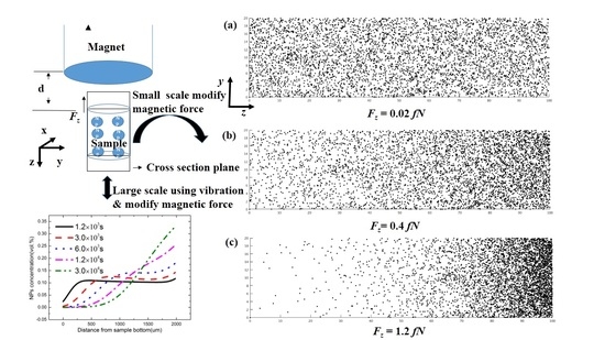
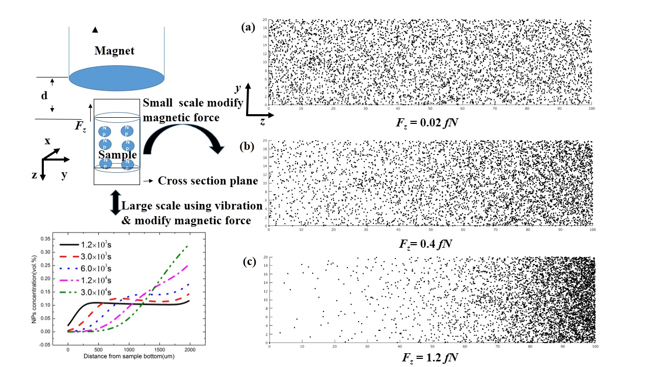
As shown in Figure 1a, we can see that with the distance changing from 1 mm to 5 mm causes the magnetic field strength under the magnet to drop markedly, and the magnetic force on the nanoparticle (NP) decreases sharply, from 1.2 fN to 0.01 fN. Figure 1b,c shows the axial force and radial force distributions at different positions under the magnet. It can be seen that the radial force is very small compared with the axial force in the center region. The force will decrease in the axial direction, but will increase in the radial direction. Therefore, the magnetic force is determined by both the external magnetic field and the distance from the sample to the magnet. We completed three simulations of both one dimension and two dimensions using three different magnetic forces: 0.02 fN, 0.4 fN, and 1.2 fN. According to the magnetic force calculation of Equation (9), a magnetic force of 1.2 fN is the point at 1 mm under magnet. As shown in Figure 1d, the magnetic force is so large that the particle can almost be assembled in the right half of the sample. If the magnetic force is smaller (0.4 fN), due to the diffusion effect, the stable particle concentration gradually grows, from left to right. If the magnetic force is smaller than 0.02 fN, there is almost no change in the particle concentration in the sample. To compare the results with the experiment, we changed the particle concentration to the numbers of particles existing in the domain (Figure 2). The distribution of particles in Figure 2a–c comes from the assumption that the magnetic force only exists in the z direction; thus, the distribution of the cross-section of the sample (the plane perpendicular to the x direction) can be simplified to a one-dimensional model, which corresponds with the distribution in Figure 1d. It is easy to see the difference among the three states, and the results of the three different concentration distributions were consistent with experiments.
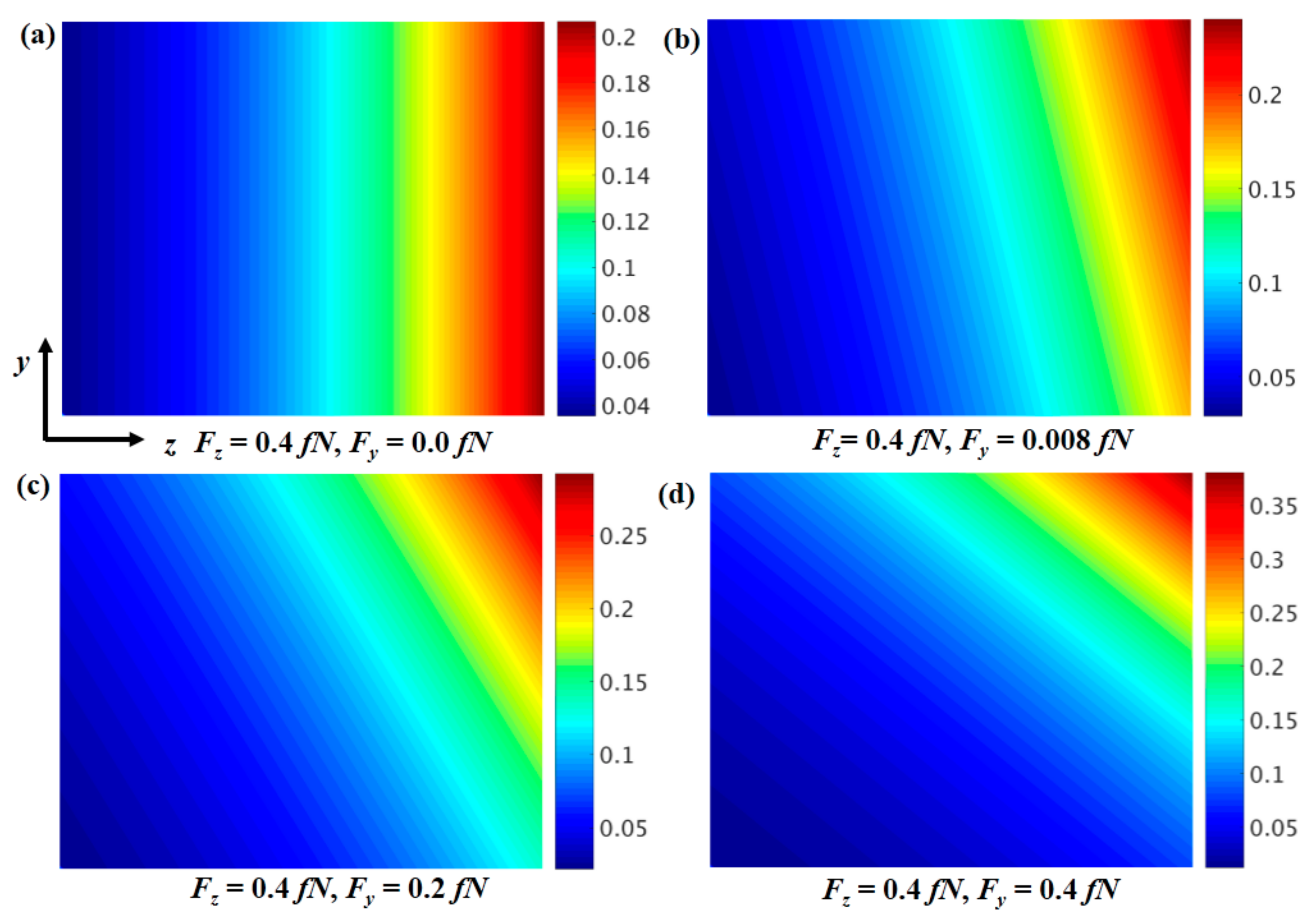
It is obvious that if the sample under the magnet is not at the center point, there will be a radial force, as seen in Figure 1c. Here, we consider the sample close to the magnet as having both the radial and axial force components. For simplicity, we assume that the magnetic force is constant in the y and z directions to study magnetic particle accumulation evolution. In Figure 3, the particle concentration shows high inhomogeneity when the force exists in both the z and y directions. If the force component in the y direction is zero, the accumulation will only exist in the z direction. If the force in the y direction is small (Figure 3b), accumulation in the y direction will exist. Due to the drift in the z and y directions, most magnetic particles will accumulate in the upper right corner. When the force in the y direction increases, the accumulation in the upper right corner will be larger, until it is sufficient to destroy the concentration gradient and mechanics gradient. This is the reason why in experiments, a larger cylindrical magnet is needed to make the magnetic force homogeneous in the sample in the y direction (radial direction) [21]. However, it is interesting that by adjusting the magnetic force in the z and y directions, one can precisely control the highly inhomogeneous or particular magnetic particle concentration distributions, and thus the high mechanics inhomogeneity in a more complex design.
As the sample scale increases, the diffusion process will not be the dominant process, and the magnetic force will change at different positions of the sample. Therefore, the force will gradually decrease when the distance from the magnet increases. Here, we consider the distance between the sample and the bottom of magnet as 2 mm. The scales of the samples are changed from 200 μm to 2 mm; other parameters used are the same as those listed in Table 1.
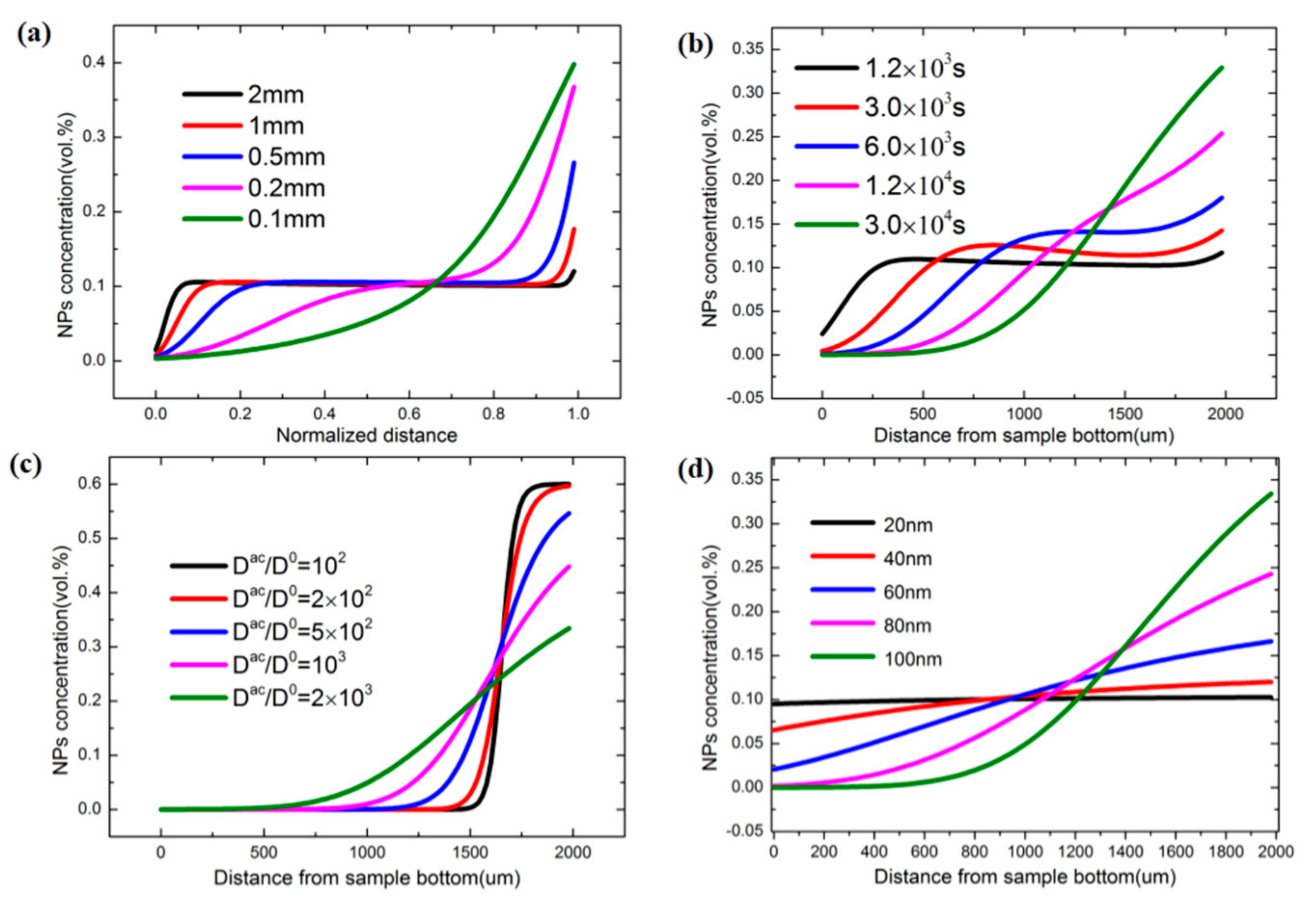
As shown in Figure 4, when the scale is small, a gradient distribution of concentration will be formed due to the diffusion process. However, when the size scale increases (e.g., 2 mm), the magnetic force will be the dominant driving force. A particle will be driven to the left side, where the magnetic force is larger than that on the other side of the sample. Another important problem is that particle accumulation is much slower than in a small-scale case. As seen from Figure 4a (2 mm case), the gradient distribution of the whole scale is difficult to obtain.
We derived the gradient concentration distribution in large-scale sample, and several points should be noted. First, the diffusion process should be accelerated, which is the reason why, in an experiment, the mechanical vibrations that can accelerate the diffusion process are needed. Second, the force should be increased to accelerate the accumulation process, and it can be described as:
Increasing the radius or magnetic field gradient can increase the magnetic force. For verification, we increased the diffusion process speed 2000 times, and increased the radius of the magnetic particle to 100 nm. For the 2-mm size scale, the result can be seen in Figure 4b; the gradient distribution of nanoparticles will be obtained at 3 × 10⁴ s. For comparison, we fixed the particle radius and accelerated the diffusion process using different times (in Figure 4c). The drift process dominates the evolution, and most particles will be driven to the right side of the sample. As the diffusion constant is gradually increased, the diffusion process competed with the drift process. A gradient concentration will be formed when the acceleration is sufficiently large. Similarly, the radius of the nanoparticles was increased, from 20 nm to 100 nm, and the diffusion constant was fixed. As shown in Figure 4d, the force was small due to the smaller particle size, and the diffusion process was the dominant process. As a nanoparticle increases in size, the driving force also increases, and the stable gradient state forms in some specific cases.
Theoretical predictions indicated that, for the material compositions adopted in this study, the FGNCs should be able to be scaled up to ~200 μm using a realistic magnetic field and processing duration. For larger length scales, such as millimeters to even centimeters, the concept of FGNCs still works; however, the material parameters (e.g., particle size, viscosity of resin matrix, etc.) and the processing conditions (e.g., magnetic field intensity, processing duration, etc.) need to be adjusted in order to achieve an optimal concentration gradient. Additionally, the method of layer-by-layer deposition, as presented by Libanori et al. [32], may be combined with FGNCs to create large objects with continuous and significant mechanical gradients.
4. Conclusions
A drift-diffusion model with a high particle concentration was proposed to study the concentration evolution of the magnetic nanoparticles under magnetic force, and the three stable states obtained from the simulations were consistent with experiments. In addition, the size effect of the sample was also studied, and it was found that large-scale gradient distribution of magnetic particles can be obtained by precisely adjusting the diffusion process and the drift process. Increasing the magnetic force and diffusion constant will enable gradient distribution in large-scale samples. The two-dimensional model also demonstrated that the nanoparticle concentrations can be highly inhomogeneous. The results showed that drift-diffusion can be an effective model to predict and design functional gradient concentrations of magnetic-responsive nanoparticles.
Acknowledgments
This work is supported by the National Natural Science Foundation of China (11504020, 11174030, 11602177), the Fundamental Research Funds for the Central Universities (FRF-TP-16-064A1).
Author Contributions
Xingqiao Ma and Houbing Huang conceived and designed the research; Xiaoming Shi completed the simulation and analysis; Zhengzhi Wang provided the experiments result and data; Xiaoming Shi wrote the paper; All contributed the discussion and revision of manuscript.
Conflicts of Interest
The authors declare no conflict of interest. The founding sponsors had no role in the design of the study; in the collection, analyses, or interpretation of data; in the writing of the manuscript, and in the decision to publish the results.
Appendix A
In two-dimensional calculations, both the radial and axial force components are computed by [30]:
The magnet is modeled as an equivalent current source, and the field distribution can be obtained via superposition (Furlani [29]). If the magnet is magnetized to saturation Ms, and centered on the z axis with its top surface at z = 0, its field is given by:
where
where K(k) and E(k) are the complete elliptic integrals of the first and second kind, respectively.
where
The field components are computed using numerical integration. The gradient of the field needs to be calculated to acquire the force, which is given by:
The magnetic force is computed by substituting Equation (A6) into Equation (A1).
References
- Barthelat, F.; Yin, Z.; Buehler, M.J. Structure and mechanics of interfaces in biological materials. Nat. Rev. Mater. 2016, 1, 16007. [Google Scholar] [CrossRef]
- Dunlop, J.W.; Weinkamer, R.; Fratzl, P. Artful interfaces within biological materials. Mater. Today 2011, 14, 70–78. [Google Scholar] [CrossRef]
- Ruiz-Molina, D.; Novio, F.; Roscini, C. Bio-and Bioinspired Nanomaterials; John Wiley & Sons: Hoboken, NJ, USA, 2014. [Google Scholar]
- Seidi, A.; Ramalingam, M.; Elloumi-Hannachi, I.; Ostrovidov, S.; Khademhosseini, A. Gradient biomaterials for soft-to-hard interface tissue engineering. Acta Biomater. 2011, 7, 1441–1451. [Google Scholar] [CrossRef] [PubMed]
- Plouffe, B.D.; Murthy, S.K.; Lewis, L.H. Fundamentals and application of magnetic particles in cell isolation and enrichment: A review. Rep. Prog. Phys. 2014, 78, 016601. [Google Scholar] [CrossRef] [PubMed]
- Ariga, K. Interfaces working for biology: Solving biological mysteries and opening up future nanoarchitectonics. ChemNanoMat 2016, 2, 333–343. [Google Scholar] [CrossRef]
- Osaki, T.; Takeuchi, S. Artificial cell membrane systems for biosensing applications. Anal. Chem. 2016, 89, 216–231. [Google Scholar] [CrossRef] [PubMed]
- Komiyama, M.; Yoshimoto, K.; Sisido, M.; Ariga, K. Chemistry can make strict and fuzzy controls for bio-systems: DNA nanoarchitectonics and cell-macromolecular nanoarchitectonics. Bull. Chem. Soc. Jpn. 2017. [Google Scholar] [CrossRef]
- Pandian, G.N.; Sugiyama, H. Nature-inspired design of smart biomaterials using the chemical biology of nucleic acids. Bull. Chem. Soc. Jpn. 2016, 89, 843–868. [Google Scholar] [CrossRef]
- Barnes, W.J.P.; Goodwyn, P.J.P.; Nokhbatolfoghahai, M.; Gorb, S.N. Elastic modulus of tree frog adhesive toe pads. J. Comp. Physiol. A Neuroethol. Sens. Neural Behav. Physiol. 2011, 197, 969–978. [Google Scholar] [CrossRef] [PubMed]
- Bar-On, B.; Barth, F.G.; Fratzl, P.; Politi, Y. Multiscale structural gradients enhance the biomechanical functionality of the spider fang. Nat. Commun. 2014, 5. [Google Scholar] [CrossRef] [PubMed]
- Lichtenegger, H.C.; Schöberl, T.; Ruokolainen, J.T.; Cross, J.O.; Heald, S.M.; Birkedal, H.; Waite, J.H.; Stucky, G.D. Zinc and mechanical prowess in the jaws of nereis, a marine worm. Proc. Natl. Acad. Sci. USA 2003, 100, 9144–9149. [Google Scholar] [CrossRef] [PubMed]
- Rogers, J.A.; Someya, T.; Huang, Y. Materials and mechanics for stretchable electronics. Science 2010, 327, 1603–1607. [Google Scholar] [CrossRef] [PubMed]
- Mei, H.; Landis, C.M.; Huang, R. Concomitant wrinkling and buckle-delamination of elastic thin films on compliant substrates. Mech. Mater. 2011, 43, 627–642. [Google Scholar] [CrossRef]
- Zhang, S.; Sun, D.; Fu, Y.; Du, H. Recent advances of superhard nanocomposite coatings: A review. Surf. Coat. Technol. 2003, 167, 113–119. [Google Scholar] [CrossRef]
- Carvalho, R.M.; Manso, A.P.; Geraldeli, S.; Tay, F.R.; Pashley, D.H. Durability of bonds and clinical success of adhesive restorations. Dent. Mater. 2012, 28, 72–86. [Google Scholar] [CrossRef] [PubMed]
- De Munck, J.D.; Van Landuyt, K.; Peumans, M.; Poitevin, A.; Lambrechts, P.; Braem, M.; Van Meerbeek, B. A critical review of the durability of adhesion to tooth tissue: Methods and results. J. Dent. Res. 2005, 84, 118–132. [Google Scholar] [CrossRef] [PubMed]
- Zeng, W.; Shu, L.; Li, Q.; Chen, S.; Wang, F.; Tao, X.M. Fiber-based wearable electronics: A review of materials, fabrication, devices, and applications. Adv. Mater. 2014, 26, 5310–5336. [Google Scholar] [CrossRef] [PubMed]
- Autumn, K.; Liang, Y.A.; Hsieh, S.T.; Zesch, W.; Chan, W.P.; Kenny, T.W.; Fearing, R.; Full, R.J. Adhesive force of a single gecko foot-hair. Nature 2000, 405, 681–685. [Google Scholar] [PubMed]
- Imbeni, V.; Kruzic, J.; Marshall, G.; Marshall, S.; Ritchie, R. The dentin–enamel junction and the fracture of human teeth. Nat. Mater. 2005, 4, 229–232. [Google Scholar] [CrossRef] [PubMed]
- Wang, Z.; Shi, X.; Huang, H.; Yao, C.; Xie, W.; Huang, C.; Gu, P.; Ma, X.; Zhang, Z.; Chen, L.-Q. Magnetically actuated functional gradient nanocomposites for strong and ultra-durable biomimetic interfaces/surfaces. Mater. Horiz. 2017. [Google Scholar] [CrossRef]
- Fletcher, D. Fine particle high gradient magnetic entrapment. IEEE Trans. Magn. 1991, 27, 3655–3677. [Google Scholar] [CrossRef]
- Furlani, E.P. Particle transport in magnetophoretic microsystems. In Microfluidic Devices in Nanotechnology: Fundamental Concepts; Wiley: New York, NY, USA, 2010; pp. 215–262. [Google Scholar]
- Furlani, E.P. Magnetic biotransport: Analysis and applications. Materials 2010, 3, 2412–2446. [Google Scholar] [CrossRef]
- Khashan, S.A.; Elnajjar, E.; Haik, Y. Numerical simulation of the continuous biomagnetic separation in a two-dimensional channel. Int. J. Multiph. Flow 2011, 37, 947–955. [Google Scholar] [CrossRef]
- Khashan, S.A.; Haik, Y. Numerical simulation of biomagnetic fluid downstream an eccentric stenotic orifice. Phys. Fluids 2006, 18, 113601. [Google Scholar] [CrossRef]
- Khashan, S.A.; Elnajjar, E.; Haik, Y. Cfd simulation of the magnetophoretic separation in a microchannel. J. Magn. Magn. Mater. 2011, 323, 2960–2967. [Google Scholar] [CrossRef]
- Furlani, E.; Ng, K. Nanoscale magnetic biotransport with application to magnetofection. Phys. Rev. E 2008, 77, 061914. [Google Scholar] [CrossRef] [PubMed]
- Furlani, E.P.; Xue, X. Field, force and transport analysis for magnetic particle-based gene delivery. Microfluid. Nanofluid. 2012, 13, 589–602. [Google Scholar] [CrossRef]
- Furlani, E.P. Permanent Magnet and Electromechanical Devices: Materials, Analysis, and Applications; Academic Press: Cambridge, MA, USA, 2001. [Google Scholar]
- Cai, L.-H.; Panyukov, S.; Rubinstein, M. Mobility of nonsticky nanoparticles in polymer liquids. Macromolecules 2011, 44, 7853–7863. [Google Scholar] [CrossRef] [PubMed]
- Libanori, R.; Erb, R.M.; Reiser, A.; Le Ferrand, H.; Süess, M.J.; Spolenak, R.; Studart, A.R. Stretchable heterogeneous composites with extreme mechanical gradients. Nat. Commun. 2012, 3, 1265. [Google Scholar] [CrossRef] [PubMed]
Figure 1.
(a) Magnetic field and force distribution in the z direction of magnet; (b,c) magnetic force in the axial and radial directions in different locations; (d) concentration distribution after 1.2 × 10³ s with different applied forces.
Figure 1.
(a) Magnetic field and force distribution in the z direction of magnet; (b,c) magnetic force in the axial and radial directions in different locations; (d) concentration distribution after 1.2 × 10³ s with different applied forces.
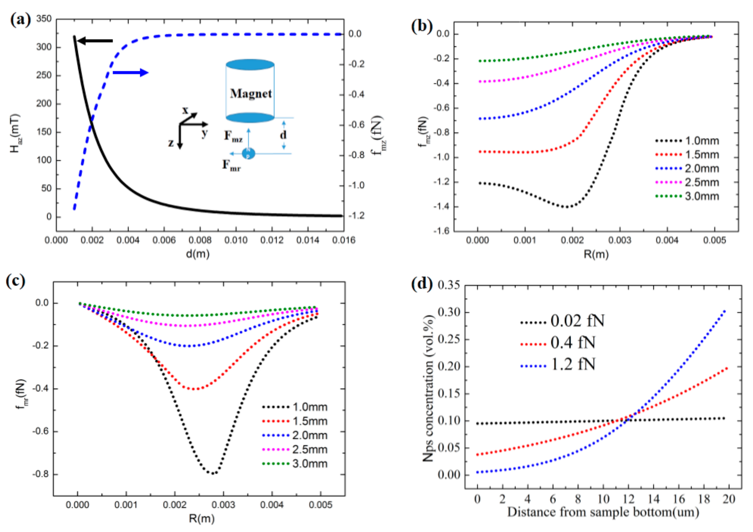
Figure 2.
(a) Cross section of the nanoparticles (NPs) distribution in the sample after 1.2 × 10³ s evolution when the magnetic force is 0.02 fN; (b) the gradient concentration distribution under the force of 0.4 fN after 1.2 × 10³ s evolution; (c) the over-accumulation state when the magnetic force is 1.2 fN after 1.2 × 10³ s evolution.
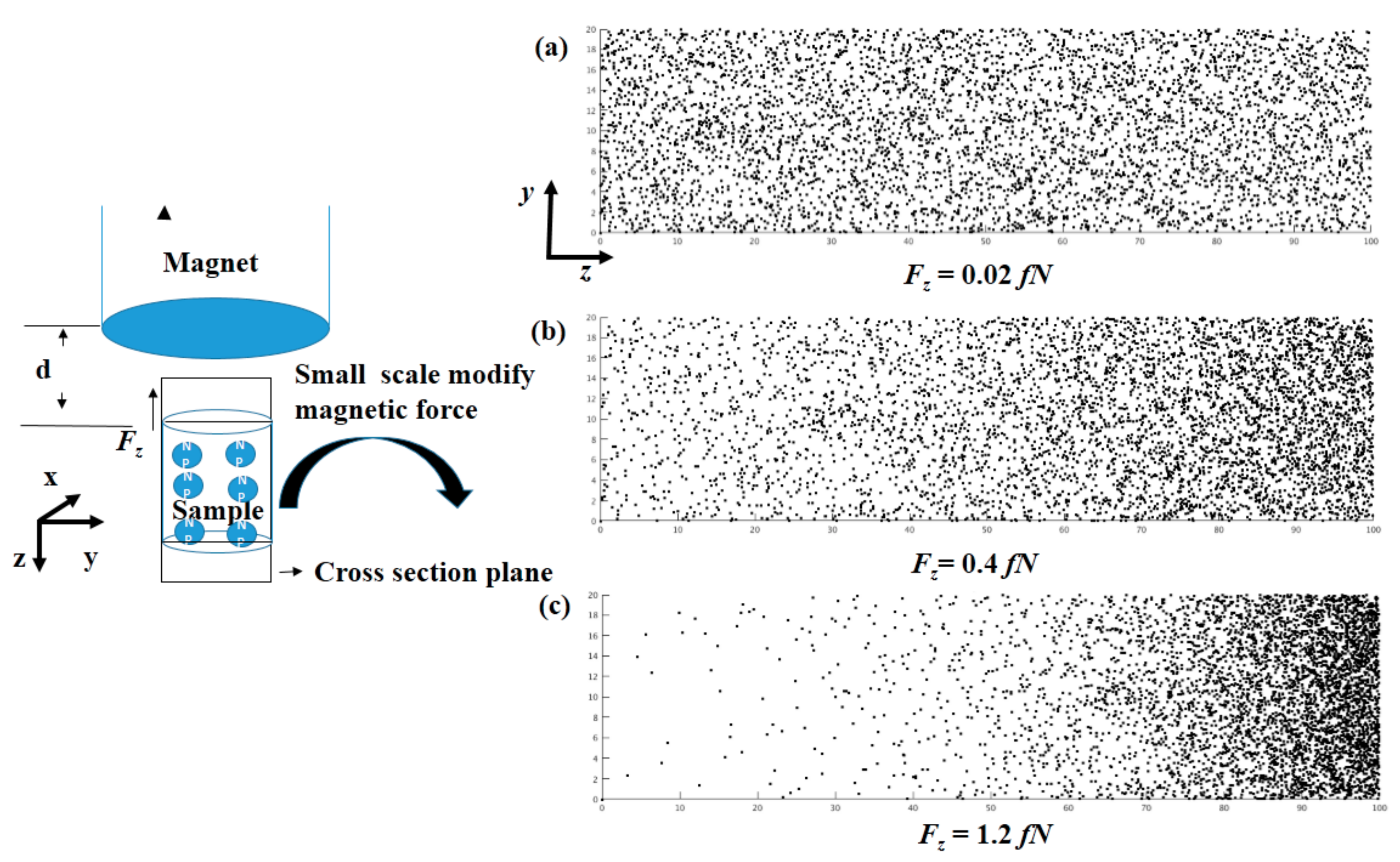
Figure 3.
Two-dimensional nanoparticle concentration distributions after 1.2 × 10³ s when the force in the z direction is fixed with 0.4 fN and the force in the y direction is selected as (a) 0, (b) 0.008 fN, (c) 0.2 fN, and (d) 0.4 fN.
Figure 3.
Two-dimensional nanoparticle concentration distributions after 1.2 × 10³ s when the force in the z direction is fixed with 0.4 fN and the force in the y direction is selected as (a) 0, (b) 0.008 fN, (c) 0.2 fN, and (d) 0.4 fN.

Figure 4.
(a) Nanoparticle concentration along the normalized distance (e.g., distance from sample bottom divided by sample thickness) for sample thicknesses ranging between 0.1 and 2.0 mm at a sufficiently long processing duration of 1.2 × 10⁴ s; (b) real-time evolution of the particle concentrations for a 2.0-mm (2000 μm) thick sample when the diffusion constant is 2000 times larger, and the magnetic particle radius is 100 nm; (c) nanoparticle concentration evolution after 1.2 × 10⁴ s when particle size is fixed, and the diffusion constant is changed; (d) nanoparticle concentration evolution after 1.2 × 10⁴ s when the diffusion constant is fixed, and the nanoparticle radius is changed.

Table 1.
Simulation parameters.
| Temperature T (K) | Magnet Length Lm (mm) | Magnet Radius Rm (mm) | Time Step dt (s) | Grid Size dx (m) |
|---|---|---|---|---|
| 300.0 | 5.0 | 3.0 | 6 × 10⁻⁴ | 2 × 10⁻⁷–2 × 10⁻⁵ |
| Fluid Viscosity η (Ns/m2) | Magnet Saturation Magnetization Ms (A/m) | Particle Saturation Magnetization Msp (A/m) | Particle Radius Rp (nm) | |
| 0.225 | 9.55 × 10⁵ | 4.78 × 10⁵ | 15.0 | |
© 2017 by the authors. Licensee MDPI, Basel, Switzerland. This article is an open access article distributed under the terms and conditions of the Creative Commons Attribution (CC BY) license (http://creativecommons.org/licenses/by/4.0/).
Share and Cite
MDPI and ACS Style
Shi, X.; Huang, H.; Wang, Z.; Ma, X. Simulation of Magnetically-Actuated Functional Gradient Nanocomposites. Appl. Sci. 2017, 7, 1171. https://doi.org/10.3390/app7111171
AMA Style
Shi X, Huang H, Wang Z, Ma X. Simulation of Magnetically-Actuated Functional Gradient Nanocomposites. Applied Sciences. 2017; 7(11):1171. https://doi.org/10.3390/app7111171
Chicago/Turabian StyleShi, Xiaoming, Houbing Huang, Zhengzhi Wang, and Xingqiao Ma. 2017. "Simulation of Magnetically-Actuated Functional Gradient Nanocomposites" Applied Sciences 7, no. 11: 1171. https://doi.org/10.3390/app7111171
Note that from the first issue of 2016, this journal uses article numbers instead of page numbers. See further details here.