Input–Output Finite Time Stabilization of Time-Varying Impulsive Positive Hybrid Systems under MDADT

1
School of mathematics and statistics, Xidian University, Xi’an 710126, China
2
School of Science, Xi’an Polytechnic University, Xi’an 710048, China
*
Author to whom correspondence should be addressed.
†
These authors contributed equally to this work.
Appl. Sci. 2017, 7(11), 1187; https://doi.org/10.3390/app7111187
Submission received: 31 August 2017
/
Revised: 23 October 2017
/
Accepted: 7 November 2017
/
Published: 17 November 2017
(This article belongs to the Special Issue Modeling, Simulation, Operation and Control of Discrete Event Systems)
Abstract
:Time-varying impulsive positive hybrid systems based on finite state machines (FSMs) are considered in this paper, and the concept of input–output finite time stability (IO-FTS) is extended for this type of hybrid system. The IO-FTS analysis of the single linear time-varying system is given first. Then, the sufficient conditions of IO-FTS for hybrid systems are proposed via the mode-dependent average dwell time (MDADT) technique. Moreover, the output feedback controller which can stabilize the non-autonomous hybrid systems is derived, and the obtained results are presented in a linear programming form. Finally, a numerical example is provided to show the theoretical results.
1. Introduction
Hybrid systems play an important role in practical applications, such as intelligent transportation systems and manufacturing systems. In fact, hybrid systems are formed by the discrete event dynamical subsystem and the continuous variable dynamical subsystem that interact and intermix with each other [1,2]. Generally, the former can be modeled as a Petri net [3,4], or a finite state machine (FSM) [5,6]. Some basic research results on FSMs have been obtained [6,7,8], concerning its structure, stability, observability, and liveliness.
If hybrid systems consist of a family of dynamical subsystems and a switching signal which determines the switching manner between the subsystems, they are called switched systems [9,10,11]. A system is positive if for any nonnegative initial condition its state variables and outputs naturally take non-negative values for all nonnegative times. Generally, positive systems have many special and interesting properties [12,13,14,15]. Moreover, positive switched systems switch between several positive subsystems [16]. The importance of positive switched systems has received much attention due to their broad applications in communication systems [17], formation flying [18], systems theory [19], and so on. Actually, the study of positive switched systems is more challenging than that of general switched systems because the features of positive systems and the features of switched systems have to be combined to obtain elegant results [20]. It should be pointed out that many previous results on positive switched systems focus mainly on stability analysis and controller synthesis [21,22,23,24,25,26,27,28,29], such as exponential stability [21,22,23,24,25], asymptotic stability [26], finite time stability (FTS) [27,28], and input–output finite time stability (IO-FTS) [30].
If the state of a system does not exceed a prescribed threshold during a fixed finite-time interval, then the system is said to have FTS [31]. This is different from Lyapunov asymptotic stability. Obviously, a finite-time stable system may not have Lyapunov stability, and a Lyapunov stable system may not be finite-time stable. The study of FTS is useful for dealing with the behavior of a system within a finite time interval. Much work on FTS has been done [27,28,31,32,33]. Furthermore, input-to-state FTS [34], robust-FTS [35] and IO-FTS [29,30,36,37,38] have also been investigated. In particular, in [27,28], the FTS is investigated with respect to positive switched linear systems by designing average dwell time (ADT) as the switching strategy.
The ADT approach is proposed and used to investigate the stability and stabilization problems for time-dependent hybrid systems [39,40]. Recently, a new switching strategy called the mode-dependent average dwell time (MDADT) technique was proposed [41]. It allows each mode in the underlying systems to have its own ADT, therefore, it is more applicable in practice than the ADT technique. Based on the MDADT technique, the periodic switching law was designed for periodic switching systems in order to achieve optimal switching control [42]. This technique is also used to deal with the stability and stabilization problems of positive switched systems [23].
The concept of IO-FTS was proposed for a linear time-varying system in [37]. Roughly speaking, a system is said to have IO-FTS if, given a class of norm bounded input signals over a specified time interval , the outputs of the system do not exceed an assigned threshold during . The author of [37] points out that IO-FTS is dependent on IO stability, because it involves signals defined over a finite-time interval, does not require the inputs and outputs to belong to the same class, and quantitative bounds on both inputs and outputs must be specified. Based on [37], some research results were derived. In [38], the IO-FTS was studied for a class of impulsive dynamical linear systems, and both static output and state feedback controllers were designed to stabilize the impulsive systems. In [43], using coupled differential linear matrix inequality, a pair of necessary and sufficient conditions for the IO-FTS of impulsive linear systems were proposed. By applying the MDADT technique, the IO-FTS was considered for a class of discrete-time positive switched systems with delays [30] and a class of continuous-time positive switched systems with delays [29] respectively, and the sufficient conditions were presented to guarantee the systems had IO-FTS. However, the IO-FTS of positive hybrid systems based on FSM was not mentioned.
Compared with some positive hybrid systems, time-varying impulsive positive hybrid systems are more general, and the existence of impulse makes it more practical. In addition, the concept of IO-FTS is defined with the finite-time interval, and the transient performance of the system can be obtained with this interval. In practical systems, the system performance is usually only concerned with the finite-time, for example, multiple guided missiles transmission, and so on. Therefore, the research on the IO-FTS of the time-varying impulsive positive hybrid systems has certain practical value and theoretical significance.
Motivated by the above backgrounds, we consider a class of hybrid systems whose discrete event subsystem is modeled as an FSM, and the continuous variable subsystem consists of several continuous time-varying impulsive positive systems. Such systems are called hybrid systems based on FSM. In fact, they are event-driven systems. The main contributions of this paper are given as follows: firstly, the concept of IO-FTS is extended for such hybrid systems. Secondly, under two different classes of exogenous input signals, the sufficient conditions of IO-FTS of a single linear system are deduced by co-positive Lyapunov function. Furthermore, by combining the multiple co-positive Lyapunov functions and MDADT technique, the sufficient conditions of IO-FTS of hybrid systems are derived, and they have good flexibility and weak conservatism. Next, the output feedback controller for stabilization problem is also deduced, and the obtained results are presented under linear programming form. Finally, a numerical example is given to ensure the accuracy of the results.
Our work is organized as follows: in Section 2, some definitions and FSM are introduced, and the problems which will be dealt with are stated. In Section 3, four theorems of IO-FTS for time-varying positive linear systems are derived and the corresponding proofs are given. In Section 4, four theorems of IO-FTS for time-varying positive hybrid systems are derived and the corresponding proofs are given. In Section 5, an example is given to show the effectiveness of the theorem. Some conclusions are given in Section 6.
Notation: Throughout our paper, denotes the set of nonnegative real numbers, represents the vector of n-tuples of real numbers, is the space of matrices with real entries, and denotes an identity matrix. For a given matrix , stands for the element in ith row and jth column of A, and () means all elements of A are positive (nonnegative), i.e., (). () means all elements of A are negative (non-positive), i.e., (). A matrix A is called a Metzler matrix if its off-diagonal elements are all nonnegative real numbers. The symbol denotes the space of vector-valued signals whose p-th power is absolutely integrable over . The restriction of to is denoted by . Given a set , a vector-valued function and a vector-valued signal , the weighted norm is denoted by .
2. Problem Formulation and Preliminaries
2.1. FSM
In this section, the FSM and the related definitions will be introduced.
Consider the FSM described by
where , , and are, respectively, the discrete state, the input event and the output of FSM at time , and is the jumping instant. , and are the finite sets of states, input events and outputs, respectively. is the FSM transition function, is the function specifying the possible events, and is the output function. is the continuous system state, , and is the current node of FSM.
Remark 1.
Note that the state transitions of the hybrid systems depend on the current node evolution of FSM, and the current node specifies the corresponding subsystem of continuous dynamics being active. means there is no jumping, and means the object will jump from the current node to another.
Remark 2.
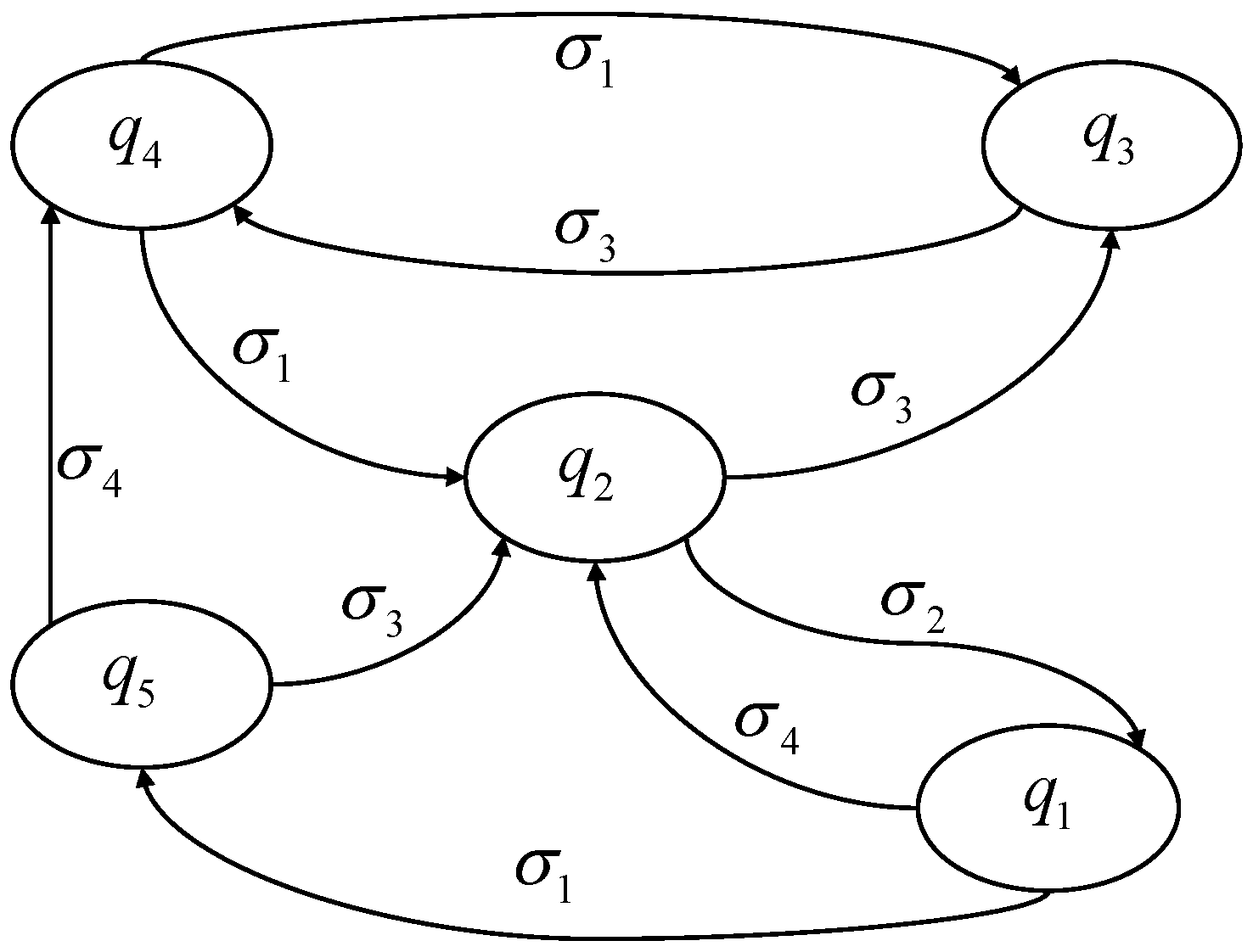
From (1), it can be seen that the state transition may be not unique when a deterministic input event occurs. This type of FSM is the non-deterministic FSM, which can be described by a state transition graph. For example, Figure 1 shows an FSM with five nodes, where the set of node is , and the set of the input event is . The jumping rule of FSM is that the current node jumps from one node to another when a particular input event occurs. However, there may be more than one node that the current node could jump to, thus, except the jump which is needed, all other jumps should be limited via controlling. After the jump, the limitation should be released to maintain the liveliness of FSM. For the FSM shown in Figure 1, the current node is , and when the input event occurs, the current node jumps from node to , then the current node is . At this time, if the input event occurs, the current node can jump from to or to . The jump from to can be limited, and then the current node jumps from to . After that, the limitation will be released.
Definition 1.
Given FSM (1) and any , if there is an input event sequence resulting in the current node jumping along the node sequence , where , and , then the node sequence is called the path from to . The jumping number ℓ is the length of the path from to . Let denote the set of all paths from node to . If the path has the least number of nodes, then it is called the shortest path from to . Furthermore, the length of the shortest path from to is called the distance from to , and it can be denoted by . In the case that there is no path from to , the distance is denoted by , .
Remark 3.
Since the directionality property of FSM is considered in the distance from to , generally, .
Next, let us introduce the distance from one node to a subset which denotes a specified subset of . We call subset E the desired set of FSM.
Definition 2.
Given FSM (1) and a desired set E, the value is called the distance from to E, and the corresponding path is called the shortest path from to E, . If , then . If there is no path from to E, then .
Definition 3.
Given FSM (1), a desired set E, and node , if
- (1)
- there is a shortest path from to E, and the current node jumps along this path; and
- (2)
- there is a positive integer , for any , ;
then the FSM is stable with regard to (w.r.t.) .
2.2. IO-FTS
Consider the following impulsive hybrid systems:
where is the system state, is the particular exogenous input, and is the system output. , , , and are continuous matrix-valued functions. is an FSM which is introduced in Section 2.1, and is the current node.
Definition 4
Lemma 1
Lemma 2
([23]). A matrix is a Metzler matrix if and only if there exists a positive constant δ such that .
Let us extend the definition of IO-FTS given in [37] to the impulsive hybrid systems previously introduced.
Definition 5.
Given a positive scalar T, a positive integer , the initial node , the desired set E, and a vector-valued function , the positive hybrid systems (2) are said to be IO-FTS w.r.t. if
- (1)
- the FSM is stable w.r.t. , , and
- (2)
- ,
where ω are a class of particular exogenous input signals defined over , and .
In this paper, two different classes of exogenous input signals are considered (as has been done in [37]), and the vector-valued function always satisfies for .
- (1)
- The set coincides with the set of norm-bounded integrable signals over , defined as follows:.
- (2)
- The set coincides with the set of uniformly bounded signals over , defined as follows:.
The definitions of and depend on the choice of , T, and , but these arguments will be omitted for brevity in the rest of the paper.
Consider a class of impulsive hybrid systems:
where is the control input, and is continuous matrix-valued function.
Given a positive scalar T and a class of particular exogenous input signals defined over , the objective of the paper is to find a output feedback control law , where is the control gain, such that the closed-loop system
is positive and there is IO-FTS w.r.t. , where , E is a desired set of FSM (1), , and .
Definition 6
([44]). For an FSM and any , let denote the number of node in the switched sequence over the interval , and let denote the total activated time of node over the interval , . We say that FSM has an MDADT , if there exist positive numbers (we call is the mode-dependent chatter bounds) and such that
3. Single Linear System
Before dealing with the IO-FTS of hybrid systems, let us first consider a single linear time-varying system which is described as follows:
where is the system state, is the particular exogenous input, is the control input, and is the output. , , , and are continuous matrix-valued functions.
The problem which will be solved is the design a state feedback control law for system (6), such that the closed-loop system
is positive and there is IO-FTS w.r.t. , where , is the control gain, and T is a positive scalar.
3.1. Stability of Autonomous System
When is a zero matrix, and the system (6) is autonomous, , then the following theorems are obtained.
Theorem 1.
The constants are with , and vector-value function . If there exist vector-valued functions and such that
- (1)
- ,
- (2)
- ,
- (3)
- ,
- (4)
- , and
- (5)
- ,
hold, then the system (6) is positive and there is IO-FTS w.r.t. , where is a Metzler matrix-valued function, , , , , and .
Proof.
When is a Metzler matrix-valued function, and , system (6) is positive by Lemma 1. Choosing co-positive Lyapunov function
according to conditions (1) and (2) of Theorem 1, we get
Due to , ,
therefore,
From condition (5) of Theorem 1,
Then the system (6) is positive and there is IO-FTS w.r.t. in the sense of Definition 4 and Definition 5. ☐
Remark 4.
Compared with Lemma 2 in [42], there are more adjustable parameters in the conditions of Theorem 1, and therefore, the conditions of Theorem 1 are more flexible.
When the parameter in Theorem 1 , the following corollary can be easily obtained.
Corollary 1.
The constants are , with , and vector-value function . If there exists a vector-valued function such that
- (1)
- ,
- (2)
- , and
- (3)
- ,
hold, then system (6) is positive and there is IO-FTS w.r.t. , where is a Metzler matrix-valued function, , , , , and .
Theorem 2.
The constants are with , and vector-value function . If there exist vector-valued functions and , such that
- (1)
- ,
- (2)
- ,
- (3)
- ,
- (4)
- , and
- (5)
- ,
hold, then system (6) is positive and there is IO-FTS w.r.t. , where is a Metzler matrix-valued function, , , , , , and .
Proof.
When is a Metzler matrix-valued function and , system (6) is positive by Lemma 1. Choose
According to the proof process of Theorem 1, for any , , and , we can obtain
From condition (5) of Theorem 2,
then
Thus system (6) is positive and there is IO-FTS w.r.t. in the sense of Definitions 4 and 5. ☐
3.2. Stabilization of Non-Autonomous Systems
When is a non-zero matrix, and system (6) is non-autonomous, the following theorems are obtained.
Theorem 3.
The constants are , with , and vector-value function . If there exist vector-valued functions and such that
- (1)
- ,
- (2)
- ,
- (3)
- ,
- (4)
- ,
- (5)
- , and
- (6)
- ,
Proof.
From Lemma 2 and condition (1) of Theorem 3, we know is a Metzler matrix, , , and , which means system (7) is positive. Then, under the control law , replacing in Theorem 1 with , we can get condition (2) of Theorem 3. Therefore, system (7) is positive, there is IO-FTS w.r.t. , and system (6) is positive and stabilizable. ☐
Theorem 4.
The constants are with , and the vector-value function . If there exist vector-valued functions and such that
- (1)
- ,
- (2)
- ,
- (3)
- ,
- (4)
- ,
- (5)
- , and
- (6)
- ,
By similar analysis of Theorem 3, we can obtain the desired results.
4. Hybrid Systems
The results of IO-FTS for single linear system are obtained in Section 3. However, if the system is not a single linear system, but is an impulsive positive hybrid system based on FSM, the research on IO-FTS of such systems is as follows in this section.
Assume that the following assumption is always satisfied in the subsequent discussion.
Assumption 1.
Given an FSM and the desired set E, for initial node , the path from to E always exists, i.e., .
For an FSM, define , , and , where is the number of the node jumping in desired set E over . For example, desired set , if the node jumping sequence is , then .
4.1. Stability of Autonomous Hybrid Systems
Firstly, consider the case where the impulsive positive hybrid systems (2) based on FSM are autonomous.
Theorem 5.
The constants are , with , and suppose E is the desired set. If there exists a vector-valued function such that
- (1)
- is strictly monotonically decreasing w.r.t. k,
- (2)
- ,
- (3)
- ,
- (4)
- , and
- (5)
- ,
hold, then system (2) is positive and there is IO-FTS w.r.t. under MDADT
where is a Metzler matrix-valued function, , , , , , , and .
Proof.
Firstly, we shall prove the stability of FSM. From Assumption 1, we know that the shortest path from to E exists. Meanwhile, , and . According to condition (1) of Theorem 5, is strictly monotonically decreasing w.r.t. k, i.e., is strictly monotonically increasing w.r.t. k. Therefore, the condition (2) of Definition 3 is satisfied. Meanwhile, , and . Because is an integer, the integer must exist, and . When the , condition (1) of Theorem 5 implies that is strictly monotonically decreasing w.r.t. k, so condition (1) of Definition 3 is satisfied. When , the condition (1) of Theorem 5 implies that is strictly monotonically decreasing w.r.t. k, i.e., is strictly monotonically increasing w.r.t. k, so the condition (2) of Definition 3 is satisfied. Thus, the FSM is stable w.r.t. , and condition (1) of Definition 5 is satisfied.
Now, we shall prove the stability of continuous dynamics. Since is a Metzler matrix-valued function, , , and . System (2) is positive by Lemma 1. Choose a co-positive type Lyapunov function . According to conditions (2) and (3) of Theorem 5, for any , we have , and
Noticing that condition (4) of Theorem 5 and integrating (14) between and t, we obtain
According to the MDADT (13), Definition 6, and ,
From condition (5) of Theorem 5, we know
and then the condition (2) of Definition 5 is satisfied.
Thus, the system (2) is positive and there is IO-FTS in the sense of Definitions 4 and 5. ☐
Remark 5.
We note that the MDADT (13) depends on the parameter . When , obviously, . This can prevent the hybrid systems from exhibiting Zeno behavior ([41]). If , then , that is to say, the jump can be arbitrary.
Theorem 6.
The constants are , with , and suppose E is the desired set. If there exists a vector-valued function such that
- (1)
- is strictly monotonically decreasing w.r.t. k,
- (2)
- ,
- (3)
- ,
- (4)
- , and
- (5)
- ,
hold, then system (2) is positive and there is IO-FTS w.r.t. under MDADT
where is a Metzler matrix-valued function, , , , , , , and .
Proof.
The proof of the stability for FSM is the same as that of Theorem 5, thus, condition (1) of the Definition 5 is satisfied.
Now, let us discuss the stability of the continuous dynamics. From the proof process of Theorem 5, we know the system (2) is positive, and
Because of and MDADT (17), we can get
From condition (5) of Theorem 6, we know
and then the condition (2) of Definition 5 is satisfied.
Thus, the system (2) is positive and there is IO-FTS in the sense of the Definitions 4 and 5. ☐
4.2. Stabilization of Non-Autonomous Hybrid Systems
Next, consider the case where impulsive positive hybrid systems (3) based on FSM are non-autonomous. Designing the output feedback controller and taking it into systems (3), then the closed-loop systems (4) can be obtained.
Theorem 7.
The constants are , with , and suppose E is the desired set. If there exists a vector-valued function such that
- (1)
- is strictly monotonically decreasing w.r.t. k,
- (2)
- ,
- (3)
- ,
- (4)
- ,
- (5)
- , and
- (6)
- ,
Proof.
From Lemma 2 and condition (2) of Theorem 7, we know is a Metzler matrix, , , , and for each . According to Lemma 1, system (4) is positive. Then, under the output feedback controller , replacing in Theorem 5 with , condition (3) of Theorem 7 can be obtained. By Theorem 5, we can easily find that system (4) is positive and there is IO-FTS w.r.t. under MDADT (13). Therefore, system (3) is positive and stabilizable. ☐
Theorem 8.
The constants are , with , and suppose E is the desired set. If there exists a vector-valued function such that
- (1)
- is strictly monotonically decreasing w.r.t. k,
- (2)
- ,
- (3)
- ,
- (4)
- ,
- (5)
- , and
- (6)
- ,
By similar analysis of Theorem 7, Theorem 8 can be easily proved.
Remark 6.
Compared with the literature [28], the MDADT technique is used for Theorems 5–8 in this paper. It allows every node of FSM to have its own ADT, therefore, the sufficient conditions of IO-FTS have good flexibility and weak conservatism.
5. Numerical Example
In this section, a numerical example is presented via MATLAB to verify the effectiveness of the theoretical results in Section 4.
Consider the time-varying impulsive positive hybrid systems based on FSM in form (3), where FSM is reported in Figure 1, , and . The system matrices are , , , , , , , , , , , , , .
The desired set is and particular exogenous input . Let , , , , , , , , and . From condition (1) of Theorem 7, the evolution path of current node of FSM can be obtained as . According to the conditions of Theorem 7 and MDADT (13), applying the linear matrix inequality (LMI) Control Toolbox and the linear programming toolbox in MATLAB, the following results can be obtained: , , , , , , , and .
The node and node are not in the evolution path. That is to say, the continuous subsystems at node and node are not activated, so they are not mentioned.
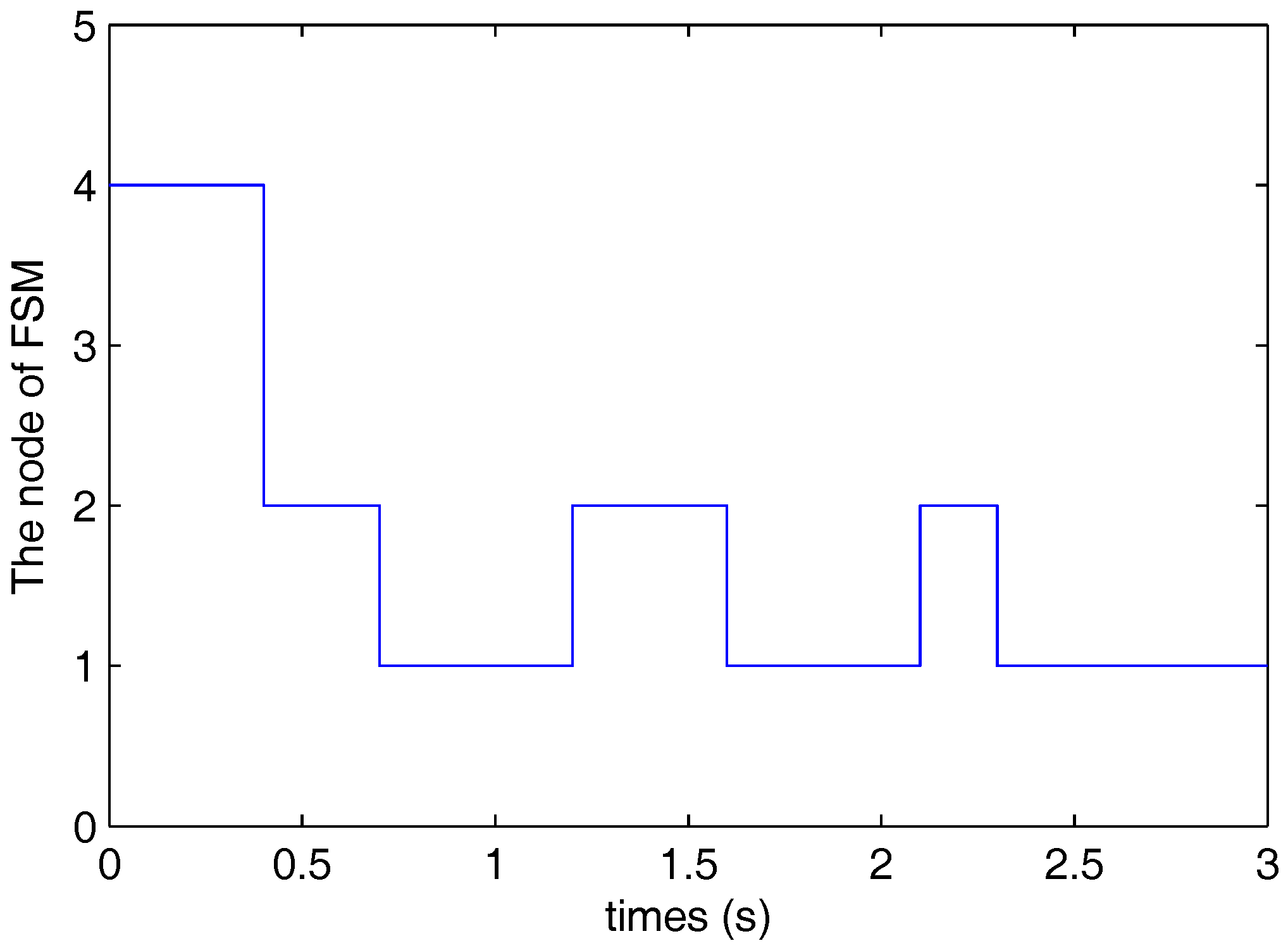
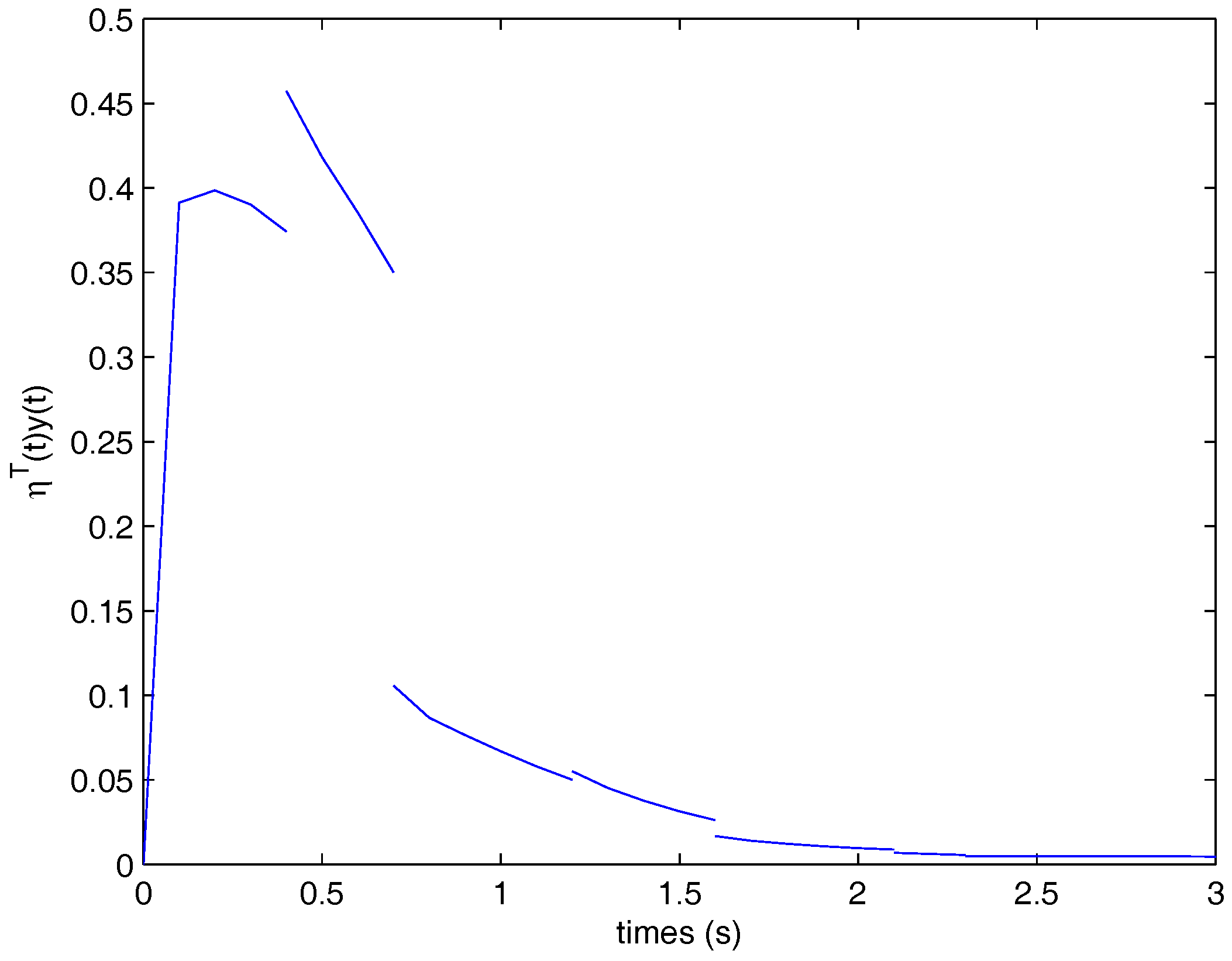
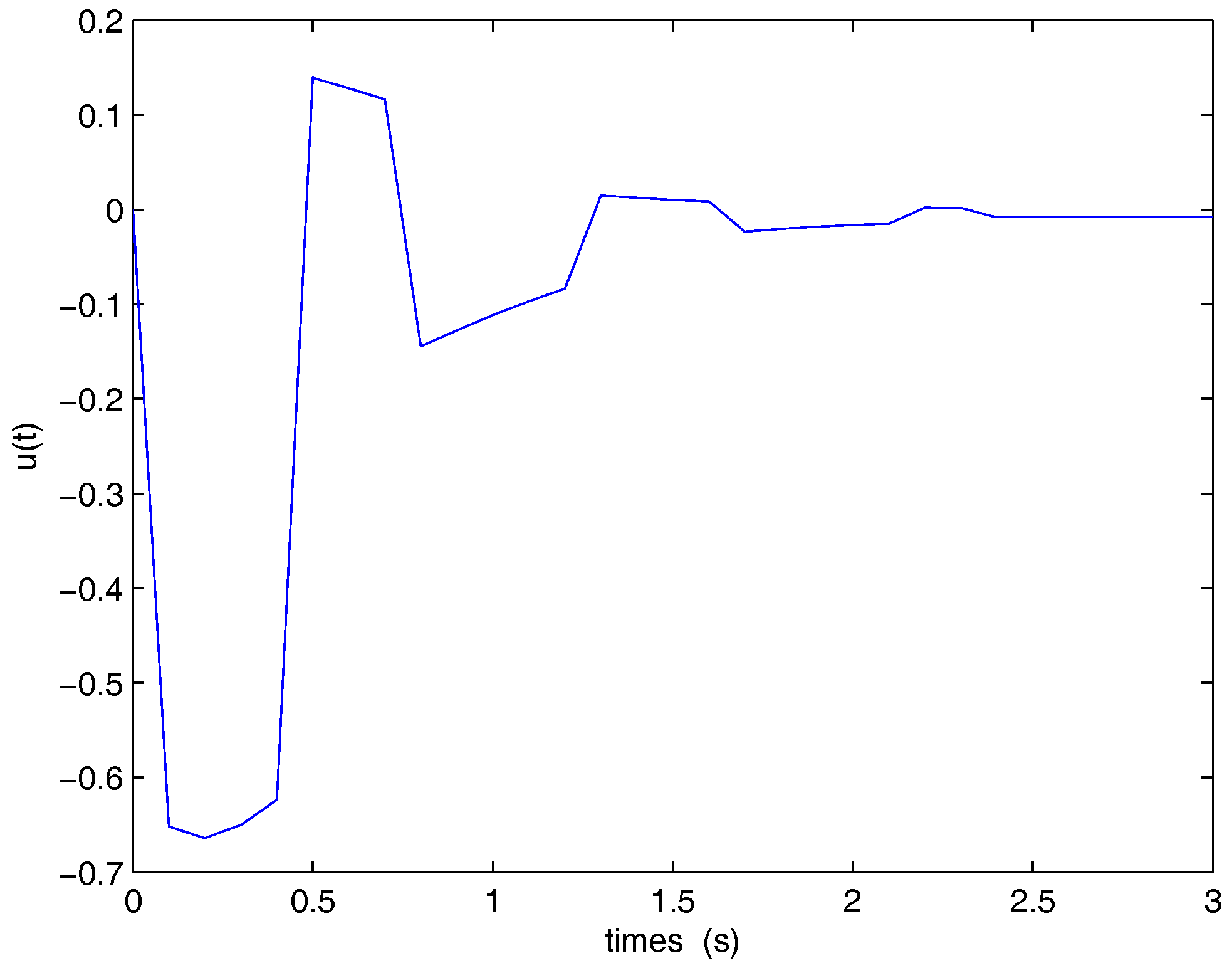
The simulation results are obtained by MATLAB. The current node evolution of FSM is shown in Figure 2, where of the y-axis represent the nodes , respectively. Obviously, the average dwell time of every node is different and satisfies MDADT (13), and the FSM is stable w.r.t. . The trajectory of output and the trajectory of the system state are shown in Figure 3 and Figure 4. Because the systems are impulsive positive hybrid systems, these trajectories are positive and have impulses. Moreover, the trajectory of output and , therefore, the given hybrid systems are positive and there is IO-FTS w.r.t. () in the sense of Definition 5. In Figure 5, the evolution of the control input is shown, and it is not always positive. Thus, the Theorem 7 is effective.
6. Conclusions
In this paper, the stability and stabilization of time-varying impulsive positive hybrid systems based on FSM have been studied. First we consider the case where there is only one time-varying positive linear system, and the stability and the state feedback controller are easily obtained. Then, we extend it to the case with time-varying impulsive positive hybrid systems based on FSM, and the stability is also obtained and proved. Furthermore, the output feedback controller is derived to stabilize the systems. The simulation results show the feasibility and effectiveness of the proposed results.
As Cyber-Social-Physical Spaces (CSPS) [45] is essentially a hybrid system, the proposed method in the paper may be applied in the CSPS or the Cyber Physical System (CPS). This will be an interesting direction in the future.
Acknowledgments
This work is supported by the National Natural Science Foundation of China (No. 61573013) and by the Doctoral Scientific Research Foundation of Xi’an Polytechnic University(BS15027).
Author Contributions
Junmin Li: Contributed to the conception of the study, the data collection and analysis, the technical guidance and technical review, and modify and finalize the final version. Lihong Yao: Contributed to the literature search, the data collection and analysis, the study program design, the technique problems, the manuscript preparation and revision, and the simulation experiment design.
Conflicts of Interest
The authors declare no conflict of interest.
Abbreviations
The following abbreviations are used in this manuscript:
| FSM | finite state machine |
| FTS | finite time stability |
| IO-FTS | input-output finite time stability |
| MDADT | mode-dependent average dwell time |
| LMI | linear matrix inequality |
References
- Branicky, M.S. Multiple Lyapunov fuctions and other analysis tools for switched and hybrid systems. IEEE Trans. Autom. Control 1998, 43, 475–482. [Google Scholar] [CrossRef]
- Chen, G.P.; Yang, Y.; Li, J.M. Finite time stability of a class of hybrid dynamical systems. IET Control Theory Appl. 2012, 6, 8–13. [Google Scholar] [CrossRef]
- Lu, X.; Zhou, M.; Ammari, A.C.; Ji, J. Hybrid Petri Nets for Modeling and Analysis of Microgrid Systems. IEEE CAA J. Autom. Sin. 2016, 3, 347–354. [Google Scholar]
- Wu, N.Q.; Zhou, M.C.; Li, Z.W. Short-Term Scheduling of Crude-Oil Operations: Enhancement of Crude-Oil Operations Scheduling Using a Petri Net-Based Control-Theoretic Approach. IEEE Robot. Autom. Mag. 2015, 22, 64–76. [Google Scholar] [CrossRef]
- Kobayashi, K.; Imura, J.; Hiraishi, K. Stabilization of finite automata with application to hybrid systems control. Discret. Event Dyn. Syst. Theory Appl. 2011, 21, 519–545. [Google Scholar] [CrossRef]
- Ozveren, C.M.; Willsky, A.S.; Antsaklis, P.J. Stability and stabilizability of discrete event dynamic systems. J. Assoc. Comput. Mach. 1991, 38, 730–752. [Google Scholar] [CrossRef]
- Ozveren, C.M.; Willsky, A.S. Observability of discrete event dynamic systems. IEEE Trans. Autom. Control 1990, 35, 797–806. [Google Scholar] [CrossRef]
- Balluchi, A.; Benvenuti, L.; Benedetto, M.D.; Sangiovanni-Vincentelli, A. Design of observers for hybrid systems. In Hybrid Systems: Computation and Control (HSCC 02), LNCS. 2289; Tomlin, C.J., Greenstreet, M.R., Eds.; Springer: Berlin, Germany, 2002; pp. 76–89. [Google Scholar]
- Yang, Y.; Chen, G.P. Finite-time stability of fractional order impulsive switched systems. Int. J. Robust Nonlinear Control 2015, 25, 2207–2222. [Google Scholar] [CrossRef]
- Gao, R.; Liu, X.Z.; Yang, J.L. On optimal control problems of a class of impulsive switching systems with terminal states constraints. Nonlinear Anal. 2010, 73, 1940–1951. [Google Scholar] [CrossRef]
- Zhao, X.D.; Shi, P.; Yin, Y.F. New Results on Stability of Slowly Switched Systems: A Multiple Discontinuous Lyapunov Function Approach. IEEE Trans. Autom. Control 2017, 62, 3502–3509. [Google Scholar] [CrossRef]
- Farina, L.; Rinaldi, S. Positive Linear Systems; Wiley: New York, NY, USA, 2000. [Google Scholar]
- Benzaouia, A.; Oubah, R. Stability and stabilization by output feedback control of positive Takagi-Sugeno fuzzy discrete-time systems with multiple delays. Nonlinear Anal. Hybrid Syst. 2014, 11, 154–170. [Google Scholar] [CrossRef]
- Wang, C.H.; Huang, T.M. Static output feedback control for positive linear continuous-time systems. Int. J. Robust Nonlinear Control 2013, 23, 1537–1544. [Google Scholar] [CrossRef]
- Haddad, W.M.; Chellaboina, V. Stability theory for nonnegative and compartmental dynamical systems with time delay. Syst. Control Lett. 2004, 51, 355–361. [Google Scholar] [CrossRef]
- Wang, J.; Zhao, J. Stabilisation of switched positive systems with actuator saturation. IET Control Theory Appl. 2016, 10, 717–723. [Google Scholar] [CrossRef]
- Shorten, R.; Leith, D.; Foy, J.; Kilduff, R. Towards an analysis and design framework for congestion control in communication networks. In 12th Yale Workshop on Adaptive & Learning Systems; Yale University: New Haven, CT, USA, 2003. [Google Scholar]
- Jadbabaie, A.; Lin, J.; Morse, A.S. Coordination of groups of mobile autonomous agents using nearest neighbor rules. IEEE Trans. Autom. Control 2003, 48, 988–1001. [Google Scholar] [CrossRef]
- Kaczorek, T. The choice of the forms of Lyapunov functions for a positive 2D Roesser model. Int. J. Appl. Math. Comput. Sci. 2007, 17, 471–475. [Google Scholar] [CrossRef]
- Margaliot, M.; Branicky, M.S. Nice reachability for planar bilinear control systems with applications to planar linear switched systems. IEEE Trans. Autom. Control 2009, 54, 1430–1435. [Google Scholar] [CrossRef]
- Xiang, M.; Xiang, Z.R. Stability, L1-gain and control synthesis for positive switched systems with time-varying delay. Nonlinear Anal. Hybrid Syst. 2013, 9, 9–17. [Google Scholar] [CrossRef]
- Zhao, X.D.; Zhang, L.X.; Shi, P.; Liu, M. Stability of switched positive linear systmes with average dwell time switching. Automatica 2012, 48, 1132–1137. [Google Scholar] [CrossRef]
- Zhang, J.; Han, Z.; Zhu, F.; Huang, J. Stability and stabilization of positive switched systems with mode-dependent average dwell time. Nonlinear Anal. Hybrid Syst. 2013, 9, 42–55. [Google Scholar] [CrossRef]
- Zhao, X.D.; Zhang, L.X.; Shi, P. Stability of a class of switched positive linear time-delay systems. Int. J. Robust Nonlinear Control 2013, 23, 578–589. [Google Scholar] [CrossRef]
- Liu, S.L.; Xiang, Z.R. Exponential L1 output tracking control for positive switched linear systems with time-varying delays. Nonlinear Anal. Hybrid Syst. 2014, 11, 118–128. [Google Scholar] [CrossRef]
- Liu, X.W.; Dang, C.Y. Stability analysis of positive switched linear systems with delays. IEEE Trans. Autom. Control 2011, 56, 1684–1690. [Google Scholar] [CrossRef]
- Xiang, M.; Xiang, Z.R. Finite-time L1 control for positive switched linear systems with time-varying delay. Commun. Nonlinear Sci. Numer. Simul. 2013, 18, 3158–3166. [Google Scholar] [CrossRef]
- Chen, G.P.; Yang, Y. Finite-time stability of switched positive linear systems. Int. J. Robust Nonlinear Control 2014, 24, 179–190. [Google Scholar] [CrossRef]
- Liu, L.; Cao, X.; Fu, Z.; Song, S. Input-Output Finite-Time Control of Positive Switched Systems with Time-Varying and Distributed Delays. J. Control Sci. Eng. 2017, 2017. [Google Scholar] [CrossRef]
- Huang, S.P.; Karimi, H.R.; Xiang, Z.R. Input-output finite-time stability of positive switched linear systems with state delays. In Proceedings of the 2013 9th Asian Control Conference (ASCC), Istanbul, Turkey, 23–26 June 2013. [Google Scholar]
- Amato, F.; Ambrosino, R.; Cosentino, C.; Tommasi, G.D. Finite-time stabilization of impulsive dynamical linear systems. Nonlinear Anal. Hybrid Syst. 2011, 5, 89–101. [Google Scholar] [CrossRef]
- Xiang, W.M.; Xiao, J.; Xiao, C.Y. Finite-time stability analysis for switched linear systems. In Proceedings of the 23rd Chinese Control and Decision Conference, Mainyang, China, 23–25 May 2011; pp. 3115–3120. [Google Scholar]
- Shen, Y.J. Finite-time control of linear parameter-varying systems with normbounded exogenous disturbance. Control Theory Appl. 2008, 6, 184–188. [Google Scholar] [CrossRef]
- Hong, Y.G.; Jiang, Z.P.; Feng, G. Finite-time input-to-state stability and application to finite-time control design. SIAM J. Control Optim. 2010, 48, 4395–4418. [Google Scholar] [CrossRef]
- Amato, F.; Ambrosino, R.; Ariola, M.; Tommasi, G.D. Robust finite-time stability of impulsive dynamical linear systems subject to norm-bounded uncertainties. Int. J. Robust Nonlinear Control 2011, 21, 1082–1092. [Google Scholar] [CrossRef]
- Huang, S.P.; Xiang, Z.R.; Karimi, H.R. Input-Output Finite-Time Stability of Discrete-Time Impulsive Switched Linear Systems with State Delays. Circuits Syst. Signal Process. 2014, 33, 141–158. [Google Scholar] [CrossRef] [Green Version]
- Amato, F.; Ambrosino, R.; Cosentino, C.; Tommasi, G.D. Input-output finite time stabilization of linear systems. Automatica 2010, 46, 1558–1562. [Google Scholar] [CrossRef]
- Amato, F.; Carannante, G.; Tommasi, G.D. Input-output finite-time stability of a class of hybrid systems via static output feedback. Int. J. Control 2011, 84, 1056–1066. [Google Scholar] [CrossRef]
- Zhang, L.; Gao, H. Asynchronously switched control of switched linear systems with acerage dwell time. Automatica 2010, 46, 953–958. [Google Scholar] [CrossRef]
- Niu, B.; Zhao, J. Stabilization and L2-gain analysis for a class of cascade switched nonlinear systems: An average dwell-time method. Nonlinear Anal. Hybrid Syst. 2011, 5, 671–680. [Google Scholar] [CrossRef]
- Ames, A.D.; Zheng, H.; Gregg, R.; Sastry, S. Is there life after Zero? Taking executions past the breaking (Zeno) point. In Proceedings of the 2006 American Control Conference, Minneapolis, MN, USA, 14–16 June 2006. [Google Scholar]
- Wang, T.; Zhang, Q.; Niu, M.Z. Optimal switching law design of periodic switching systems based on mode-dependent average dwell time. In Proceedings of the 35th Chinese Control Conference, Chengdu, China, 27–29 July 2016. [Google Scholar]
- Amato, F.; Tommasi, G.D.; Pironti, A. Input-output finite-time stabilization of impulsive linear systems: Necessary and sufficient conditions. Nonlinear Anal. Hybrid Syst. 2016, 19, 93–106. [Google Scholar] [CrossRef]
- Zhao, X.; Zhang, L.; Shi, P.; Liu, M. Stability and Stabilization of switched linear systems with mode-dependent average dwell time. IEEE Trans. Autom. Control 2012, 57, 1809–1815. [Google Scholar] [CrossRef]
- Wang, F.Y. Control 5.0: From Newton to Merton in Popper’s Cyber-Social-Physical Spaces. IEEE/CAA J. Autom. Sin. 2016, 3, 233–234. [Google Scholar]
Figure 1.
A simple example of the finite state machine (FSM).

Figure 2.
The current node evolution.

Figure 3.
The output .

Figure 4.
The trajectory of the system state.
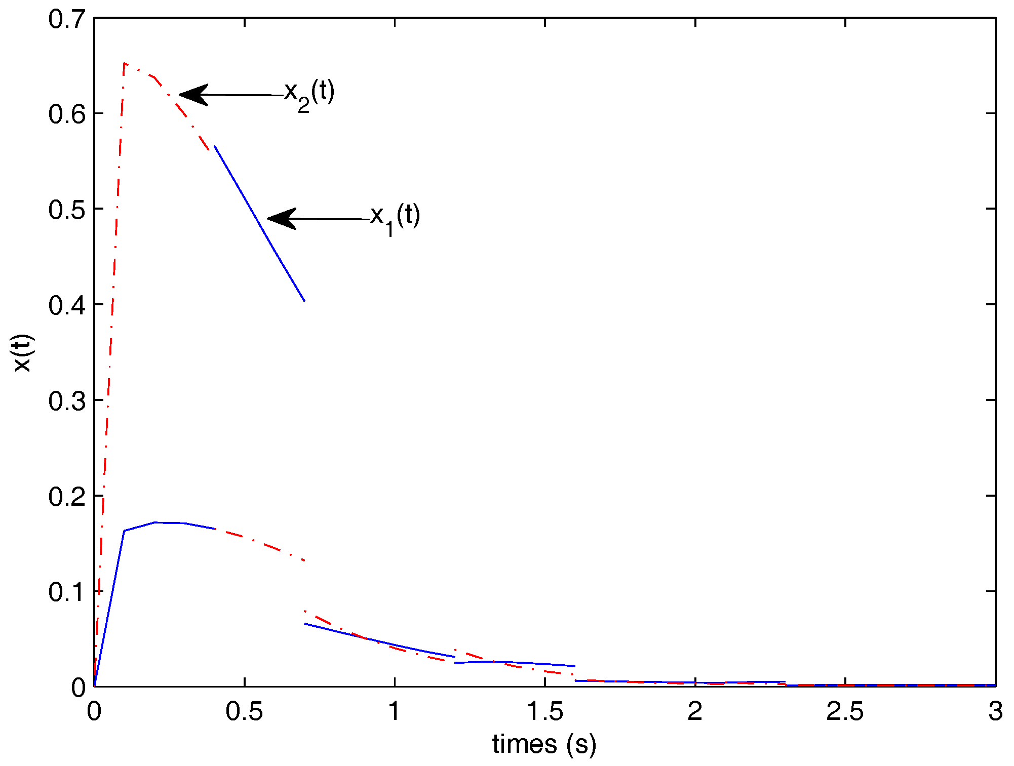
Figure 5.
The control input.

© 2017 by the authors. Licensee MDPI, Basel, Switzerland. This article is an open access article distributed under the terms and conditions of the Creative Commons Attribution (CC BY) license (http://creativecommons.org/licenses/by/4.0/).
Share and Cite
MDPI and ACS Style
Yao, L.; Li, J. Input–Output Finite Time Stabilization of Time-Varying Impulsive Positive Hybrid Systems under MDADT. Appl. Sci. 2017, 7, 1187. https://doi.org/10.3390/app7111187
AMA Style
Yao L, Li J. Input–Output Finite Time Stabilization of Time-Varying Impulsive Positive Hybrid Systems under MDADT. Applied Sciences. 2017; 7(11):1187. https://doi.org/10.3390/app7111187
Chicago/Turabian StyleYao, Lihong, and Junmin Li. 2017. "Input–Output Finite Time Stabilization of Time-Varying Impulsive Positive Hybrid Systems under MDADT" Applied Sciences 7, no. 11: 1187. https://doi.org/10.3390/app7111187
Note that from the first issue of 2016, this journal uses article numbers instead of page numbers. See further details here.