Adaptive LOS Path Following for a Podded Propulsion Unmanned Surface Vehicle with Uncertainty of Model and Actuator Saturation

Abstract

This paper addresses three related issues concerning the path following control of a podded propulsion unmanned surface vehicle (USV), namely modeling, guidance and control. The pod is different from the general propeller-rudder propulsion device, and its essence is a vector thruster. Therefore, first, through various assumptions and simplification, the three-degree of freedom (DOFs) planar motion model of the podded propulsion USV is established. Then, the classical line-of-sight (LOS) guidance strategy is improved by adaptive sideslip angle and a time-varying lookahead distance. Based on the guidance system, the corresponding controllers for yaw rate and surge speed are presented, which are combined by backstepping technology, the neural network minimum parameter learning method and the neural shunting model. Specifically, the neural network minimum parameter learning method is proposed to compensate the uncertainty of the model and the immeasurability of external disturbances, and the neural shunting model is employed to cope with the “explosion of complexity” problem of backstepping. Meanwhile, an auxiliary dynamic system is introduced to prevent actuator saturation (input saturation). All error signals of the system are proven to be uniformly ultimately bounded (UUB) by employing Lyapunov stability theory. Finally, two numerical simulations are given to prove the correctness of the proposed scheme.

1. Introduction

USV is a kind of intelligent offshore platform equipment, which has the characteristics of small volume and fast speed. It can perform tasks in harsh or dangerous environments, which can reduce unnecessary casualties [1]. Travel speed is one of the most important factors to describe the performance level of ships. Many literature works have proven that the propulsion efficiency of the pod is higher than the ordinary propeller-rudder, which can significantly improve the maneuverability and the speed of ships [2,3]. The research object of this paper is a podded propulsion USV, and based on the analysis, the thrust of the pod and the force acting on the ship hull, the three-DOF planar motion model is established by hypothesis and simplification.

The biggest advantage of USV comes from its ability for independent, autonomous travel. Meanwhile, path following is the most basic function of autonomous navigation [4]. For now, the most popular navigation algorithm to implement path following is look-ahead LOS [5,6]. The main principle of the LOS guidance algorithm is to imitate the behavior of a helmsman, which steers the vehicle towards a lookahead distance ($\Delta$) ahead of the projection point of the vehicle along the path. The characteristics of the LOS algorithm lie in that it is light in computation and easy to implement. However, the traditional LOS guidance algorithm has two shortcomings: in the path-following process, the sideslip angle will be generated due to the effects of ocean disturbances; the value of $\Delta$ is a constant, which cannot be adjusted adaptively.

To compensate for the adverse effects of sideslip angle, many efforts have been made by scholars from all over the world. Generally speaking, the simplest way is to measure the sideslip angle directly. In [7], the sideslip angle was calculated by measuring the surge and sway velocities. However, not only are the corresponding measuring instruments (sensors, etc.) expensive, but also the measured data are noisy. Another way is that an integral term was added into the classic LOS guidance algorithm, proposing integral LOS (ILOS) to alleviate the effect of sideslip angle [8]. Lekkas et al. proved that the $\kappa$-exponentially stable ILOS guidance algorithm was derived for curved paths [9]. In addition, Fossen et al. treated the sideslip angle as an unknown constant and identified its value with an online adaptive approach [10]. Meanwhile, a novel predictor-based LOS (PLOS) guidance law for the path following of the underactuated marine surface vehicle was proposed [11]. The proposed navigation strategy not only inherited the simplicity of the traditional LOS, but also ensured the fast convergence of the marine surface vehicle sideslip angle. For the issue of time-varying $\Delta$, Pavlov et al. presented a nonlinear model predictive control (MPC) approach, which can adjust its value online to achieve smaller overshoot and faster convergence speed compared with the constant $\Delta$ [12]. A function to adjust $\Delta$ according to the cross-track error was given in [13]. In [10], only the cross-track was considered, but in this note, both cross-track error and along-track error are taken into account, which is more universal. Besides, the fuzzy algorithm is adopted to optimize the value of $\Delta$. Due to its small size and high speed, USV is more susceptible to external disturbances. Therefore, both cross-track error and the differential of cross-track error are taken into account when tuning $\Delta$. The role of the differential of cross-track error is to provide an early judgment, which can enhance the robustness of the system.

Modeling, guidance and motion control are three essential elements of path following. There is very much literature investigating the design of the path following controller, and different algorithms are introduced into it, such as classic and variant PID control [13,14], fuzzy control [15], sliding mode control [16], backstepping control [17], and so on. According to engineering practice, the ship model has the characteristics of nonlinearity and uncertainty due to the continuous change of operating conditions. To deal with the uncertainty of the model problem, neural network (back propagation (BP) neural network and radial basis function (RBF) neural network) [18,19] or fuzzy logic [20,21], which have the ability of universal approximation, are usually introduced into the control system. However, fuzzy logic requires more expert prior knowledge, so the neural network is used more widely in the field of universal approximation. In [22], a new novel neural network adaptive controller was developed for cooperative path following of marine vessels. Although the neural network can solve the problem of the unknown dynamic model, as a multi-layer neural network, it will undoubtedly increase the amount of computation of the control system. Besides, in practical engineering, there is a very important factor that needs to be taken into consideration, that is the input saturation of the actuator. Input saturation is easy to ignore for the path following design since the commanded control inputs calculated by the path-following control laws are possibly constrained by the maximum outputs that the actuator can produce. If input saturation is not taken into consideration, it is very likely to reduce system performance and even lead to instability of the entire path following. In [23], an auxiliary design system was introduced to analyze the effect of input constraints, and its states were used for adaptive tracking control design. In the presence of unknown time-varying disturbances and input saturation, an auxiliary dynamic system, a disturbance observer and a dynamic surface control (DSC) technique were used to design a robust nonlinear control law for a fully-driven supply ship [24]. In [25], a path-following controller for USV was developed by combining the neural network and DSC technique subject to input saturation.

Motivated by the above-mentioned observations, the goal of this article is that based on the establishment of the podded propulsion USV model, the ALOS algorithm with a time-varying $\Delta$ is proposed to provide guidance. Besides, a path-following controller, which is proposed by using the backstepping method, the neural shunting model, the neural network minimum parameter learning method and the auxiliary dynamic system, is developed for USV without knowing the exact information of the model structure and the time-varying external disturbances. The main contributions of this note can be summarized as follows:

(1)

Based on force analysis and MMG (Ship Manoeuvring Mathematical Model Group)separation modeling theory, the podded propulsion USV is proven to be an underactuated system.

(2)

An improved LOS algorithm is employed as a navigation strategy for USV, which means that it not only ensures the expected compensation effect, but also avoids the use of expensive sensor equipment.

(3)

A novel neural shunting model is adopted to deal with the “explosion of complexity”, which can reduce the computational complexity of the control system.

(4)

Model uncertainties and time-varying external disturbances are estimated by the neural network minimum parameter learning method. Compared with RBF and BP, the neural network minimum parameter learning method has a smaller amount of computation.

(5)

The auxiliary dynamic system is introduced to prevent the input saturation problem, which is closer to practical engineering.

The rest of the paper is organized as follows. Section 2 describes the process of modeling. In Section 3, ALOS with a time-varying $\Delta$ guidance algorithm is proposed. In Section 4, the path following controller is designed. The stability of the closed-loop system is demonstrated in Section 5. In Section 6, numerical simulations are given to prove the correctness of the strategy proposed in this note. Finally, Section 7 summarizes the full text.

2. Modeling of USV

2.1. Kinematics Equation

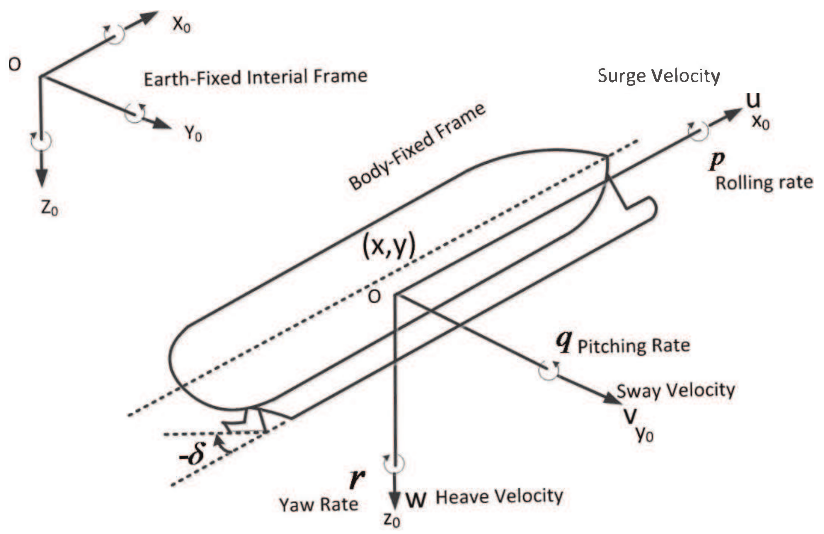
The corresponding relationship between the body-fixed frame and the Earth-fixed inertial frame is shown in Figure 1; where $o-x_0{y}_0{z}_0$ is the body-fixed frame and $O-X_0{Y}_0{Z}_0$ is the Earth-fixed inertial frame.

In practice, USV has six DOFs, including: surge velocity u, sway velocity v, yaw rate r, heave velocity w, rolling rate p and pitching rate q. Since path following is a planar motion task, only w, p and q need to be taken into account. $(x,y)$ represents the position of the USV, and $\delta$ is the propulsion angle. The kinematics equation transformation between the body-fixed frame and the Earth-fixed inertial frame can be expressed as:

$$\begin{array}{c}\hfill \dot{\zeta }=J(\psi )\upsilon \end{array}$$

(1)

where $\psi$ is the heading angle, $\zeta ={[x,y,\psi ]}^T$, $\upsilon ={[u,v,r]}^T$ and $J(\psi )$ is the transition matrix.

$$\begin{array}{c}\hfill J(\psi )=\left[\begin{array}{ccc}cos(\psi )& -sin(\psi )& 0\\ sin(\psi )& cos(\psi )& 0\\ 0& 0& 1\end{array}\right]\end{array}$$

(2)

Then, we can get the kinematics equation of USV [26].

$$\begin{array}{c}\hfill \left\{\begin{array}{c}\dot{x}=ucos\psi -vsin\psi \hfill \\ \dot{y}=usin\psi +vcos\psi \hfill \\ \dot{\psi }=r\hfill \end{array}\right.\end{array}$$

(3)

2.2. Kinetic Equation

To study the planar kinetic equation, the following standards are used: m is vehicle’s mass, $x_g$ is the distance from the barycenter of USV to the body-fixed frame, $I_z$ is the vehicle’s moment of inertia about the z-axis, $X_u$, $Y_v$, $Y_r$, $N_v$ and $N_r$ are the linear damping terms, $X_{\dot{u}}$, $Y_{\dot{v}}$, $Y_{\dot{r}}$, $N_{\dot{v}}$ and $N_{\dot{r}}$ are the hydrodynamic added mass terms. The planar kinetic equation of three DOFs is established by Lagrange mechanics theory.

$$\begin{array}{c}\hfill M\dot{\upsilon }+C(\upsilon )\upsilon +D(\upsilon )\upsilon =\tau +{\tau }_b\end{array}$$

(4)

where $\tau ={[{\tau }_u,{\tau }_v,{\tau }_r]}^T$, ${\tau }_u$, ${\tau }_v$ and ${\tau }_r$ represent the control forces and moment in all directions, ${\tau }_b={[b_u,b_v,b_r]}^T$, $b_u$, $b_v$, $b_r$ denote the external disturbances caused by wind, wave and currents, M is the inertia matrix, $C(\upsilon )$ is the Coriolis and centripetal matrix and $D(\upsilon )$ is hydrodynamic damping matrix.

$$\begin{array}{c}\hfill M=\left[\begin{array}{ccc}m-X_{\dot{u}}& 0& 0\\ 0& m-Y_{\dot{v}}& m{x}_g-Y_{\dot{r}}\\ 0& m{x}_g-Y_{\dot{r}}& I_z-N_{\dot{r}}\end{array}\right]\end{array}$$

(5)

$$\begin{array}{c}\hfill C(\upsilon )=\left[\begin{array}{ccc}0& 0& a_{13}\\ 0& 0& a_{23}\\ a_{31}& a_{32}& 0\end{array}\right]\end{array}$$

(6)

where $a_{13}=-(m-Y_{\dot{v}})v-(m{x}_g-Y_{\dot{r}})r$, $a_{23}=(m-X_{\dot{u}})u$, $a_{31}=(m-Y_{\dot{v}})v+(m{x}_g-Y_{\dot{r}})r$ and $a_{32}=-(m-X_{\dot{u}})u$.

$$\begin{array}{c}\hfill D(\upsilon )=\left[\begin{array}{ccc}-X_u& 0& 0\\ 0& -Y_v& -Y_r\\ 0& -N_v& -N_r\end{array}\right]\end{array}$$

(7)

When the propulsion angle is $\delta$, the vector thrusts in different directions are:

$$\begin{array}{c}\hfill \left\{\begin{array}{c}{\tau }_u=Tcos\delta \hfill \\ {\tau }_v=T\sin \delta \hfill \\ {\tau }_r=LT\sin \delta \hfill \end{array}\right.\end{array}$$

(8)

T is the thrust of the thruster, which is a function related to the rotating speed of the propeller. L is the length from the center of rotation to the fulcrum of the propulsor. The effective attack angle of the pod ${\alpha }_R$ is a small value with the unit “rad”. Therefore, we can draw $sin{\alpha }_R={\alpha }_R=\delta$, where the propulsion angle $\delta =$ [−0.5236 rad, 0.5236 rad] [27]. Hence, if $\delta$ is a small value and $L>1$, then ${\tau }_v\approx 0$.

Assumption 1.

For a typical pod, it can be rotated $360{}^{\circ }$. However, in order to reduce the difficulty of manipulating USV, its rotatable angle is often limited to a certain range, such as $\pm 30{}^{\circ }$.

Define $m_{11}=m-X_{\dot{u}}$, $m_{22}=m-Y_{\dot{v}}$, $m_{23}=m{x}_g-Y_{\dot{r}}$, $m_{32}=m{x}_g-N_{\dot{v}}$, $m_{33}=I_z-N_{\dot{r}}$, $d_{11}=-X_u$, $d_{22}=-Y_v$, $d_{23}=-Y_r$, $d_{32}=-N_v$, $d_{33}=-N_r$, $X_p={\tau }_u$ and $N_p={\tau }_r$. Assuming that USV is symmetrical and the barycenter of it coincides with the center of the body-fixed frame, that is to say, $x_g=0$, $Y_{\dot{r}}=0$, $N_{\dot{v}}=0$, $Y_r=0$ and $N_v=0$, then (4) can be simplified as (9).

$$\begin{array}{c}\hfill \left\{\begin{array}{c}\dot{u}=f_u+\frac{1}{m_{11}}{\tau }_u+\frac{1}{m_{11}}{b}_u\hfill \\ \dot{v}=f_v+\frac{1}{m_{22}}{b}_v\hfill \\ \dot{r}=f_r+\frac{1}{m_{33}}{\tau }_r+\frac{1}{m_{33}}{b}_r\hfill \end{array}\right.\end{array}$$

(9)

where:

$$\begin{array}{c}\hfill \left\{\begin{array}{c}{f}_u=\frac{m_{22}}{m_{11}}vr-\frac{d_{11}}{m_{11}}u\hfill \\ f_v=-\frac{m_{11}}{m_{22}}ur-\frac{d_{22}}{m_{22}}v\hfill \\ f_r=\frac{m_{11}-m_{22}}{m_{33}}uv-\frac{d_{33}}{m_{33}}r\hfill \end{array}\right.\end{array}$$

(10)

Remark 1.

From the modeling principle, many assumptions and simplifications are used; from the actual navigation, the operating conditions are constantly changing. Therefore, in essence, $f_u$, $f_v$ and $f_r$ are uncertain dynamic functions:

Remark 2.

The sway v has been proven in [28] to be passive-bounded stable.

Assumption 2.

The external disturbances accord with the following assumptions: $\left|b_u\right|\le b_{u max}$, $\left|b_v\right|\le b_{v max}$ and $\left|b_r\right|\le b_{r max}$, where $b_{u max}$, $b_{v max}$ and $b_{r max}$ are unknown positive constants.

Assumption 3.

There exist constraints on the control inputs and velocities as ${\tau }_{u min}\le {\tau }_u\le {\tau }_{u max}$, ${\tau }_{r min}\le {\tau }_r\le {\tau }_{r max}$, $u\le u_{max}$, $v\le v_{max}$ and $r\le r_{max}$ with positive constants ${\tau }_{u max}$, ${\tau }_{r max}$, $u_{max}$, $v_{max}$, $r_{max}$ and negative constants ${\tau }_{u min}$, ${\tau }_{r min}$.

3. LOS Guidance Algorithms

The LOS algorithm is used to convert the desired path to reference heading angle. Meanwhile, in order to be more universal, we assume that the sideslip angle cannot be measured directly, so the adaptive method is employed to estimate sideslip angle to compensate the difference between heading angle and course angle. Finally, the fuzzy algorithm is used to adjust the value of lookahead distance $\Delta (t)>0$ to realize a better control effect.

3.1. Problem Formulation

From Figure 2, $(x,y)$ stands for the coordinates of USV in the Earth-fixed inertial frame. In this article, we consider the path-following task at the kinematic level and assume that the speed can be manually or automatically controlled. The resultant speed of the USV is the vector sum of u and v, $U=\sqrt{u^2+v^2}$ and $U_{min}\le U\le U_{max}$, $U_{min}>0$. Consider a geometric path $(x_p(\theta ),y_p(\theta ))$ as the reference path, where $\theta$ is an independent variable. The along-track error and the cross-track error are computed as the orthogonal distance to the path-tangential reference frame defined by the point $(x_p(\theta ),y_p(\theta ))$. Hence:

$$\begin{array}{c}\hfill \left[\begin{array}{c}{x}_e\hfill \\ y_e\hfill \end{array}\right]=R^T({\gamma }_p)\left[\begin{array}{c}x-x_p(\theta )\hfill \\ y-y_p(\theta )\hfill \end{array}\right]\end{array}$$

(11)

$$\begin{array}{c}\hfill R({\gamma }_p)=\left[\begin{array}{cc}cos({\gamma }_p)& -sin({\gamma }_p)\\ sin({\gamma }_p)& cos({\gamma }_p)\end{array}\right]\end{array}$$

(12)

where $R({\gamma }_p)\in SO(2)$ is the rotation matrix in yaw.

$$\begin{array}{c}\hfill {\gamma }_p(\theta )=arctan(y_p^{\prime }(\theta ),x_p^{\prime }(\theta ))\end{array}$$

(13)

where $x_p^{\prime }(\theta )=\partial x_p/\phantom{\partial x_p{\partial }_{\theta }}{\partial }_{\theta }$ and $y_p^{\prime }(\theta )=\partial y_p/\phantom{\partial y_p\partial \theta }{\partial }_{\theta }$. Note that for a straight line, ${\gamma }_p=arctan(y_{j+1}-y_j,x_{j+1}-x_j)$ is a constant between the waypoints. The equations of the along- and the cross-track errors for a given vehicle position $(x,y)$ become:

$$\begin{array}{c}\hfill \left\{\begin{array}{c}{x}_e=(x-x_p(\theta ))cos({\gamma }_p)+(y-y_p(\theta ))sin({\gamma }_p)\hfill \\ y_e=-(x-x_p(\theta ))sin({\gamma }_p)+(y-y_p(\theta ))cos({\gamma }_p)\hfill \end{array}\right.\end{array}$$

(14)

where $x_e$ represents the along-tracking error and $y_e$ is the cross-tracking error. Differentiating $x_e$ and $y_e$ along (14) gives:

$$\begin{array}{c}\hfill {\dot{x}}_e=Ucos(\psi -{\gamma }_p+\beta )+{\dot{\gamma }}_p{y}_e-U_p\end{array}$$

(15)

where $\beta =arctan(v,u)$ denotes the sideslip angle and $U_p$ is the virtual reference speed to stabilize $x_e$.

$$\begin{array}{cc}\hfill {\dot{y}}_e=& -(\dot{x}-{\dot{x}}_p(\theta ))sin({\gamma }_p)-(x-x_p(\theta ))cos({\gamma }_p){\dot{\gamma }}_p\hfill \\ \hfill & +(\dot{y}-{\dot{y}}_p(\theta ))cos({\gamma }_p)-(y-y_p(\theta ))sin({\gamma }_p){\dot{\gamma }}_p\hfill \\ \hfill =& usin(\psi -{\gamma }_p)+vcos(\psi -{\gamma }_p)+\underset{n_1}{\underbrace{{\dot{x}}_p(\theta )sin({\gamma }_p)-{\dot{y}}_p(\theta )cos({\gamma }_p)}}\hfill \\ \hfill & +{\dot{\gamma }}_p\underset{x_e}{\underbrace{((x-x_p(\theta ))cos({\gamma }_p)+(y-y_p(\theta ))sin({\gamma }_p))}}\hfill \end{array}$$

(16)

$n_1$ can be rewritten as $n_1=\dot{\theta }\sqrt{x^{\prime }{(\theta )}^2+y^{\prime }{(\theta )}^2}sin({\gamma }_p+\varphi )$; where $\varphi =arctan(-y^{\prime }(\theta ),x^{\prime }(\theta ))=-{\gamma }_p$.

Assumption 4.

Assume that β is small, so $sin(\beta )=\beta$ and $cos(\beta )=1$. During path following, we can view β as a constant, so $\dot{\beta }=0$.

Based on the conclusions above, we can get that:

$$\begin{array}{c}\hfill {\dot{y}}_e=Usin(\psi -{\gamma }_p)+Ucos(\psi -{\gamma }_p)\beta \end{array}$$

(17)

The goal of the design is to put forward an ALOS guidance strategy, which can make the underactuated USV follow the desired geometric path $(x_p(\theta ),y_p(\theta ))$. Meanwhile, the unknown sideslip angle is compensated in real time, which is inevitable. It is worth mentioning that the ultimate goal of path following is to achieve $x_e\to 0$ and $y_e\to 0$ as $t\to \infty$.

3.2. Adaptive Compensation of the Sideslip Angle

Assumption 5.

The heading controller can follow the reference heading angle perfectly, so $\psi ={\psi }_d$. Let $\widehat{\beta }$ denote the adaptive estimate of β, and $\tilde{\beta }=\beta -\widehat{\beta }$ is the parameter estimation error.

The ALOS can be represented as (18) and (19).

$$\begin{array}{c}\hfill {\psi }_d={\gamma }_p-acrtan(\frac{1}{\Delta }{y}_e+\widehat{\beta })\end{array}$$

(18)

$$\begin{array}{c}\hfill \dot{\widehat{\beta }}=\kappa \frac{U{y}_e}{\sqrt{{\Delta }^2+{(y_e+\Delta \widehat{\beta })}^2}}\end{array}$$

(19)

For (15), the velocity $U_p$ can be seen as used to stabilize $x_e$.

$$\begin{array}{c}\hfill U_p=-U\frac{\Delta }{\sqrt{{\Delta }^2+{(y_e+\Delta \widehat{\beta })}^2}}+\gamma x_e\end{array}$$

(20)

and:

$$\begin{array}{c}\hfill \dot{\theta }=\frac{U_p}{\sqrt{{x^{\prime }}_p{(\theta )}^2+{y^{\prime }}_p{(\theta )}^2}}\end{array}$$

(21)

where $0<{\Delta }_{min}<\Delta <{\Delta }_{max}$ is the user-specified lookahead distance. Applying (17) with $0<U_{min}\le U\le U_{max}$ renders the origin $(x_e,y_e,\tilde{\beta })=(0,0,0)$ uniformly globally asymptotically stable (UGAS).

$$\begin{array}{c}\hfill sin(arctan(-\frac{y_e+\Delta \widehat{\beta }}{\Delta }))=-\frac{y_e+\Delta \widehat{\beta }}{\sqrt{{\Delta }^2+{(y_e+\Delta \widehat{\beta })}^2}}\end{array}$$

(22)

$$\begin{array}{c}\hfill cos(arctan(-\frac{y_e+\Delta \widehat{\beta }}{\Delta }))=-\frac{\Delta }{\sqrt{{\Delta }^2+{(y_e+\Delta \widehat{\beta })}^2}}\end{array}$$

(23)

Then:

$$\begin{array}{c}\hfill {\dot{y}}_e=-U\frac{y_e-\Delta \tilde{\beta }}{\sqrt{{\Delta }^2+{(y_e+\Delta \widehat{\beta })}^2}}-{\dot{\gamma }}_p{x}_e\end{array}$$

(24)

Similarly,

$$\begin{array}{c}\hfill {\dot{x}}_e={\dot{\gamma }}_p{y}_e-U\frac{\Delta }{\sqrt{{\Delta }^2+{(y_e+\Delta \widehat{\beta })}^2}}-U_p\end{array}$$

(25)

Design the Lyapunov function $V_1=\frac{1}{2}{x}_e^2+\frac{1}{2}{y}_e^2+\frac{1}{2}\kappa {\tilde{\beta }}^2$ with $\kappa >0$. From (24) and (25), we can get that:

$$\begin{array}{cc}\hfill {\dot{V}}_1=& x_e{\dot{x}}_e+y_e{\dot{y}}_e+\kappa \tilde{\beta }\dot{\tilde{\beta }}\hfill \\ \hfill =& -\gamma x_e^2-\frac{U{y}_e^2}{\sqrt{{\Delta }^2+{(y_e+\Delta \widehat{\beta })}^2}}+\tilde{\beta }(\frac{U\Delta y_e}{\sqrt{{\Delta }^2+{(y_e+\Delta \widehat{\beta })}^2}}+\frac{1}{\kappa }\dot{\tilde{\beta }})\hfill \end{array}$$

(26)

Since $\dot{\tilde{\beta }}=-\dot{\widehat{\beta }}$, we can substitute (19) into (26). This gives:

$$\begin{array}{c}\hfill {\dot{V}}_1<-\gamma x_e^2-\frac{U{y}_e^2}{\sqrt{{\Delta }^2+{(y_e+\Delta \widehat{\beta })}^2}}<0\end{array}$$

(27)

The speed of the USV is chosen as:

$$\begin{array}{c}\hfill U=l\sqrt{{\Delta }^2+{(y_e+\Delta \widehat{\beta })}^2}\end{array}$$

(28)

where $l>0$; we obtain:

$$\begin{array}{c}\hfill {\dot{V}}_1\le -\gamma x_e^2-l{y}_e^2<0\end{array}$$

(29)

Theorem 1.

The origin $(x_e,y_e,\tilde{\beta })=(0,0,0)$ is uniformly globally exponentially stable (UGES) if the adaptive law of θ is (21), ${\psi }_d$ is set as (18) and U is equal to (28).

Proof of Theorem 1

The first Lyapunov function $V_1$ is set as positive definite and radially unbounded, while its derivative is quadratically negative definite when asserting (18), (21) and (28). Therefore, by the stability theory of Lyapunov, the origin $(x_e,y_e,\tilde{\beta })=(0,0,0)$ is UGES. This is actually a theoretical conclusion. In actual engineering, due to the interference of various factors and the restriction of actual system, the result of this idea is difficult to achieve. ☐

3.3. Time-Varying Lookahead Distance

Up to now, adaptive compensation of the sideslip angle is proposed in the case of considering the value of lookahead distance $\Delta$ as constant. In principle, a smaller $\Delta$ is selected when the USV is far from the reference path, and this will produce an aggressive behavior to decrease the cross-track error faster; a larger $\Delta$ is selected when the USV is near the reference path. The fuzzy algorithm is used to optimize the value of $\Delta$, and it is a dual input and single output system: $y_e$ and ${\dot{y}}_e$ are input entries; the gain ℑ is the output entry. The final output is $\Delta ={\Delta }_{min}+\Im ({\Delta }_{max}-{\Delta }_{min})$.

The method of fuzzy optimization is shown as follows:

(1)

$y_e$ and ${\dot{y}}_e$ are normalized to $\left[\begin{array}{cc}-1& 1\end{array}\right]$; the data domain of ℑ is $\left[\begin{array}{cc}0& 1\end{array}\right]$.

(2)

$y_e$ is equally divided into NB, NS, Z, PS and PB; ${\dot{y}}_e$ is equally divided into NB, NS, Z, PS and PB; ℑ is equally divided into VS, S, M, B and VB.

(3)

Zadeh and max-min are used for fuzzy reasoning. Meanwhile, the centroid area center of gravity method is used for defuzzification.

When the fuzzy algorithm is employed to optimize $\Delta$, Equation (27) can be rewritten as:

$$\begin{array}{c}\hfill {\dot{V}}_1<-\gamma x_e^2-\frac{U{y}_e^2}{\sqrt{{{\Delta }_{max}}^2+{(y_e+{\Delta }_{max}\widehat{\beta })}^2}}<0\end{array}$$

(30)

The corresponding conclusions can be obtained from (30) that when the strategy of changing $\Delta$ is introduced into the ALOS algorithm, the region where the guidance system is UGAS is constrained by ${\Delta }_{max}$. Therefore, the larger ${\Delta }_{max}$ is, the more limited the region where the system is UGAS becomes.

4. Control System Design

$\left|•\right|$ is the absolute operator. $∥•∥$ denotes the Euclidean norm, and ${∥•∥}^2={\sum }_{c,d}{\left\{\right\}}_{c,d}^2·{(•)}_{c,d}$ denotes the element of $(•)$ in row c and column d.

4.1. Preliminary Knowledge

4.1.1. Neural Network Minimum Parameter Learning Method

In engineering applications, the RBF neural network is the most commonly-used method to address the uncertainty of models and parameters, which can represent a given continuous function $f(x)$ as:

$$\begin{array}{c}\hfill f(x)=W^{T}h(x)+\epsilon \forall x\subset {\Omega }_x\end{array}$$

(31)

where ${\Omega }_x$ is a compact set in $R^m$, weight vector $W={\left[w_1,w_2,....,w_l\right]}^T\in R^l$, $h(x)=[h_1(x),h_2(x),\cdots ,h_l(x)]$ is a Gaussian functions, $\epsilon$ is the approximation error and $\left|\epsilon \right|\le \overline{\epsilon }$, $\overline{\epsilon }>0$, $l>0$ is the node number of the neural network [29].

However, the RBF neural network increases the computational complexity of the controller. In order to simplify the control law, a novel neural network minimum parameter learning method is adopted to approximate the unknown function [30]. The essence of the neural network minimum parameter learning method is as follows: define $\phi ={∥W∥}^2$, and $\phi$ is a normal number. $\widehat{\phi }$ is the estimated value of $\phi$, and its estimation error $\tilde{\phi }=\widehat{\phi }-\phi$.

4.1.2. Neural Shunting Model

The neural shunting model was proposed by Grossberg in 1988, which was used to understand the real-time adaptive response of an individual to the outside environment. With the continuous progress of technology, the neural shunting model has been applied in many fields, such as motor control, robotic arm control, path planning, and so on. The neural shunting model can be represented as:

$$\begin{array}{c}\hfill {\dot{\beta }}_r=-A{\beta }_r+(B-{\beta }_r)f({\alpha }_r)-(D+{\beta }_r)g({\alpha }_r)\end{array}$$

(32)

where ${\alpha }_r$ and ${\beta }_r$ are the input and output of the model, respectively. A, B and D are corresponding positive design parameters. In addition, if ${\alpha }_r\ge 0$, $f({\alpha }_r)={\alpha }_r$ and $g({\alpha }_r)=0$; if ${\alpha }_r<0$, $f({\alpha }_r)=0$ and $g({\alpha }_r)=-{\alpha }_r$. In essence, the neural shunting model can be viewed as a filter, and it can make the control signal flatten.

4.1.3. Input Saturation

In practice, the control force and moment are subject to saturation nonlinearities due to the physical limitations of the actuator. It can be described as follows:

$$\begin{array}{c}\hfill {\tau }_i=\left\{\begin{array}{c}{\tau }_{i max},if{\tau }_{0i}>{\tau }_{i max}\hfill \\ {\tau }_{0i},if{\tau }_{i min}\le {\tau }_{0i}\le {\tau }_{i max}\hfill \\ {\tau }_{i min},if{\tau }_{0i}<{\tau }_{i min}\hfill \end{array}\right.\end{array}$$

(33)

where $i=u,r$, ${\tau }_{i max}$ and ${\tau }_{i min}$ are the maximum and minimum output that the actuator can provide, respectively, ${\tau }_{0i}$ is the control command without considering input saturation and ${\tau }_i$ is the final control command with the same meaning as (9).

To prevent the saturation problem of implementing agencies, an auxiliary dynamic system is constructed as follows [23]:

$$\begin{array}{c}\hfill {\dot{e}}_i=\left\{\begin{array}{c}-K_{ei}{e}_i-\frac{\left|i_e·\Delta {\tau }_i\right|+0.5\Delta {\tau }_i^2}{\left|e_i^2\right|}·e_i+\Delta {\tau }_i,\left|e_i\right|\ge {\xi }_i\hfill \\ 0,\left|e_i\right|<{\xi }_i\hfill \end{array}\right.\end{array}$$

(34)

where $K_{ei}$ is a positive design parameter, $e_i$ is an introduced variable, ${\xi }_i$ is a small positive parameter and $i_e$ is a variable, which will be introduced in the next subsection. $\Delta {\tau }_i={\tau }_i-{\tau }_{0i}$.

4.2. Yaw Rate Controller

The yaw rate controller and surge speed controller are designed to achieve the control of the heading angle and speed of USV.

Step 1: Define a heading tracking error ${\psi }_e$ as:

$$\begin{array}{c}\hfill {\psi }_e=\psi -{\psi }_d\end{array}$$

(35)

From (3) and (9), the time derivative of ${\psi }_e$ is given by:

$$\begin{array}{c}\hfill {\dot{\psi }}_e=r-{\dot{\psi }}_d\end{array}$$

(36)

In order for ${\psi }_e\to 0$, ${\alpha }_r$ is selected as the virtual control.

$$\begin{array}{c}\hfill {\alpha }_r=-k_1{\psi }_e+{\dot{\psi }}_d\end{array}$$

(37)

where $k_1$ is a positive design parameter. Make ${\alpha }_r$ pass through a neural shunting model, then one can obtain:

$$\begin{array}{c}\hfill {\dot{\beta }}_r=-A{\beta }_r+(B-{\beta }_r)f({\alpha }_r)-(D+{\beta }_r)g({\alpha }_r)\end{array}$$

(38)

The meaning of each symbol has the same meaning as those defined in (32). Define:

$$\begin{array}{c}\hfill r_e=r-{\beta }_r\end{array}$$

(39)

From (9) and (38), the time derivative of (39) is given by:

$$\begin{array}{c}\hfill {\dot{r}}_e=f_r+\frac{1}{m_{33}}{\tau }_r+\frac{1}{m_{33}}{b}_r+{\Theta }_r\end{array}$$

(40)

where ${\mathsf{\Theta }}_r=[A+f({\alpha }_r)+g({\alpha }_r)]{\beta }_r-[Bf({\alpha }_r)-Dg({\alpha }_r)]$.

The neural network minimum parameter learning method is used to estimate the uncertain function $f_r+\frac{1}{m_{33}}{b}_r$. Its approximation error is ${\epsilon }_r$, and $\left|{\epsilon }_r\right|\le {\overline{\epsilon }}_r$, ${\overline{\epsilon }}_r>0$.

The corresponding control law is chosen as:

$$\begin{array}{c}\hfill {\tau }_{0r}=-k_{re}{r}_e-m_{33}{\Theta }_r-{\psi }_e-\frac{1}{2}{r}_e{\widehat{\phi }}_r{h}^{T}h\end{array}$$

(41)

where $k_{re}$ is a positive design parameter and h is the shorthand for $h(x)$.

$$\begin{array}{c}\hfill {\dot{e}}_r=\left\{\begin{array}{c}-K_{er}{e}_r-\frac{\left|r_e·\Delta {\tau }_r\right|+0.5\Delta {\tau }_r^2}{\left|e_r^2\right|}·e_r+\Delta {\tau }_r,\left|e_r\right|\ge {\xi }_r\hfill \\ 0,\left|e_r\right|<{\xi }_r\hfill \end{array}\right.\end{array}$$

(42)

where the meaning of each symbol has the same meaning as those defined in (34). The ultimate control law for r is selected as:

$$\begin{array}{c}\hfill {\tau }_r=\left\{\begin{array}{c}{\tau }_{rmax},if{\tau }_{0r}>{\tau }_{rmax}\hfill \\ {\tau }_{0r},if{\tau }_{rmin}\le {\tau }_{0r}\le {\tau }_{rmax}\hfill \\ {\tau }_{rmin},if{\tau }_{0r}<{\tau }_{rmin}\hfill \end{array}\right.\end{array}$$

(43)

where the meaning of each symbol has the same meaning as those defined in (33).

The adaptive law of the estimation function is:

$$\begin{array}{c}\hfill {\dot{\widehat{\phi }}}_r=\frac{1}{2}{\gamma }_r{r}_e^2{h}^{T}h-{\kappa }_r{\gamma }_r{\widehat{\phi }}_r\end{array}$$

(44)

where ${\gamma }_r$ and ${\kappa }_r$ are two positive design parameters.

4.3. Surge Speed Controller

When time $t\to \infty$, the objective of the speed is $\underset{t\to \infty }{lim}U\to U_d$. Since $U=\sqrt{u^2+v^2}$, we get that $u\to \sqrt{U_d^2-v^2}$. Hence, we define a desired surge speed as $u_d\to \sqrt{U_d^2-v^2}$, which is valid when assuming $U_d\ge \left|v\right|$ at all times. This assumption is highly realistic since in practice, $\left|v\right|$ is just a small fraction of U. Then, the objective of the surge speed controller becomes $\underset{t\to \infty }{lim}u\to u_d$. Define a surge speed tracking error $u_e$ as:

$$\begin{array}{c}\hfill u_e=u-u_d\end{array}$$

(45)

Taking the time derivative of (45) along (9) yields:

$$\begin{array}{c}\hfill {\dot{u}}_e=f_u+\frac{1}{m_{11}}{\tau }_u+\frac{1}{m_{11}}{b}_u-{\dot{u}}_d\end{array}$$

(46)

Equally, the neural network minimum parameter learning method is used to approximate $f_u+\frac{1}{m_{11}}{b}_u$. Its approximation error is ${\epsilon }_u$ and $\left|{\epsilon }_u\right|\le {\overline{\epsilon }}_u$, ${\overline{\epsilon }}_u>0$.

The corresponding control law is chosen as:

$$\begin{array}{c}\hfill {\tau }_{0u}=-k_{ue}{u}_e+m_{11}{\dot{u}}_d-\frac{1}{2}{u}_e{\widehat{\phi }}_u{h}^{T}h\end{array}$$

(47)

where $k_{ue}$ is a positive design parameter.

$$\begin{array}{c}\hfill {\dot{e}}_u=\left\{\begin{array}{c}-K_{eu}{e}_u-\frac{\left|u_e·\Delta {\tau }_u\right|+0.5\Delta {\tau }_u^2}{\left|e_u^2\right|}·e_u+\Delta {\tau }_u,\left|e_u\right|\ge {\xi }_u\hfill \\ 0,\left|e_u\right|<{\xi }_u\hfill \end{array}\right.\end{array}$$

(48)

Then, the ultimate control law for u is selected as:

$$\begin{array}{c}\hfill {\tau }_u=\left\{\begin{array}{c}{\tau }_{umax},if{\tau }_{0u}>{\tau }_{umax}\hfill \\ {\tau }_{0u},if{\tau }_{umin}\le {\tau }_{0u}\le {\tau }_{umax}\hfill \\ {\tau }_{umin},if{\tau }_{0u}<{\tau }_{umin}\hfill \end{array}\right.\end{array}$$

(49)

where the meaning of each symbol has the same meaning as those defined in (33) and (34).

The adaptive law of the estimation function is:

$$\begin{array}{c}\hfill {\dot{\widehat{\phi }}}_u=\frac{1}{2}{\gamma }_u{u}_e^2{h}^{T}h-{\kappa }_u{\gamma }_u{\widehat{\phi }}_u\end{array}$$

(50)

where ${\gamma }_u$ and ${\kappa }_u$ are two positive design parameters.

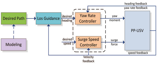
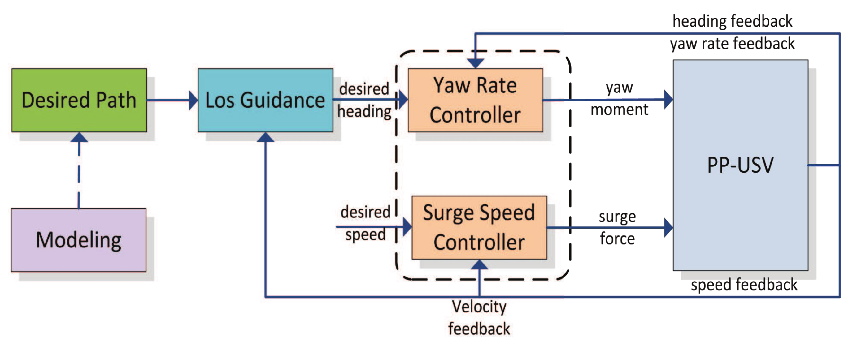
In order to facilitate the understanding of the full paper, the block diagram of the podded propulsion USV path following is shown in Figure 3.

As shown in Figure 3, the “modeling” of podded propulsion (PP) unmanned surface vehicle is the basis of the path-following system. The reason why “modeling” and “desired path” are connected by dotted lines is that the problem of model identification is not considered in this paper. Then, the “desired path” is converted into target heading by “LOS guidance”. Finally, the path following of the podded propulsion unmanned surface vehicle is implemented by designing the “yaw rate controller” and “surge speed controller” respectively.

5. Stability Analysis

5.1. Stability of the Controller

Define:

$$\begin{array}{c}\hfill y_r={\beta }_r-{\alpha }_r\end{array}$$

(51)

The time derivative of (51) is:

$$\begin{array}{cc}\hfill {\dot{y}}_r=& -([A+f({\alpha }_r)+g({\alpha }_r)]{\beta }_r-[Bf({\alpha }_r)-Dg({\alpha }_r)])-{\mathrm{X}}_r\hfill \end{array}$$

where $X_r=\frac{\partial {\alpha }_r}{\partial {\psi }_e}{\dot{\psi }}_e+\frac{\partial {\alpha }_r}{\partial {\dot{\psi }}_d}{\ddot{\psi }}_d$ and $\left|X_r\right|\le {\overline{X}}_1$, ${\overline{X}}_r>0$. Define $A_r=A+f({\alpha }_r)+g({\alpha }_r)$; then, one can obtain:

$$\begin{array}{c}\hfill {\dot{y}}_r=-A_r{\beta }_r+B{\alpha }_r-{\mathrm{X}}_r\end{array}$$

(52)

Theorem 2.

For System (9), the corresponding control laws (43), (49) and adaptive laws (44), (50) can make the signals and states of the system uniformly ultimately bounded.

Proof of Theorem 2

Define the second Lyapunov function.

$$\begin{array}{cc}\hfill V_2=& \frac{1}{2}({\psi }_e^2+m_{11}{u}_e^2+m_{33}{r}_e^2+y_r^2+\frac{1}{{\gamma }_u}{\tilde{\phi }}_u^2+\frac{1}{{\gamma }_r}{\tilde{\phi }}_r^2+e_u^2+e_r^2)\hfill \end{array}$$

(53)

The time derivative of (53) is:

$$\begin{array}{cc}\hfill {\dot{V}}_2=& {\psi }_e{\dot{\psi }}_e+m_{11}{u}_e{\dot{u}}_e+m_{33}{r}_e{\dot{r}}_e+y_r{\dot{y}}_r+\frac{1}{{\gamma }_u}{\tilde{\phi }}_u{\dot{\widehat{\phi }}}_u+\frac{1}{{\gamma }_r}{\tilde{\phi }}_r{\dot{\widehat{\phi }}}_r+e_u{\dot{e}}_u+e_r\dot{e}{}_r\hfill \end{array}$$

(54)

Substituting (43) and (49) into (54) yields; then, one can get that:

$$\begin{array}{cc}\hfill {\dot{V}}_2\le & -k_1{\psi }_e^2+{\psi }_e^2+\frac{1}{4}{y}_r^2-(k_{ue}-\frac{1}{2})u_e^2-(k_{re}-\frac{1}{2})r_e^2\hfill \\ \hfill & +{\tilde{\phi }}_u(-\frac{1}{2}{u}_e^2{h}^{T}h+\frac{1}{{\gamma }_u}{\dot{\widehat{\phi }}}_u)+{\tilde{\phi }}_r(-\frac{1}{2}{r}_e^2{h}^{T}h+\frac{1}{{\gamma }_r}{\dot{\widehat{\phi }}}_r)\hfill \\ \hfill & +y_r{\dot{y}}_r+e_u{\dot{e}}_u+e_r\dot{e}{}_r+u_e{\epsilon }_u+r_e{\epsilon }_r+u_e\Delta {\tau }_u+r_e\Delta {\tau }_r+1+\frac{1}{2}{\overline{\epsilon }}_u^2+\frac{1}{2}{\overline{\epsilon }}_r^2\hfill \end{array}$$

(55)

Substituting (44) and (50) into (55), we can obtain:

$$\begin{array}{cc}\hfill {\dot{V}}_2\le & -(k_1-1){\psi }_e^2-(k_{ue}-\frac{1}{2})u_e^2-(k_{re}-\frac{1}{2})r_e^2-\frac{1}{2}{\kappa }_u({\tilde{\phi }}_u^2-{\phi }_u^2)-\frac{1}{2}{\kappa }_r({\tilde{\phi }}_r^2-{\phi }_r^2)+y_r{\dot{y}}_r\hfill \\ \hfill & +e_u{\dot{e}}_u+e_r{\dot{e}}_r+u_e\Delta {\tau }_u+r_e\Delta {\tau }_r+1+\frac{1}{4}{y}_r^2+\frac{1}{2}{\overline{\epsilon }}_u^2+\frac{1}{2}{\overline{\epsilon }}_r^2\hfill \end{array}$$

(56)

Define $B=A_r$; then, $A_r{\beta }_r-A_r{\alpha }_r=A_r{y}_r$. (57) can be obtained.

$$\begin{array}{cc}\hfill {\dot{V}}_2\le & -(k_1-1){\psi }_e^2-(k_{ue}-\frac{1}{2})u_e^2-(k_{re}-\frac{1}{2})r_e^2-\frac{1}{2}{\kappa }_u({\tilde{\phi }}_u^2-{\phi }_u^2)-\frac{1}{2}{\kappa }_r({\tilde{\phi }}_r^2-{\phi }_r^2)-A_r{y}_r^2\hfill \\ \hfill & -y_r{X}_r+e_u{\dot{e}}_u+e_r{\dot{e}}_r+u_e\Delta {\tau }_u+r_e\Delta {\tau }_r+1+\frac{1}{4}{y}_r^2+\frac{1}{2}{\overline{\epsilon }}_u^2+\frac{1}{2}{\overline{\epsilon }}_r^2\hfill \end{array}$$

(57)

From Young’s inequality, i.e., $ab\le \frac{1}{2\sigma }{a}^2+\frac{\sigma }{2}{b}^2$ with $\sigma >0$ and $(a,b)\in {\Re }^2$, it follows that $-y_r{X}_r\le \frac{\sigma y_r^2}{2}+\frac{{\overline{X}}_r^2}{2\sigma }$. Then:

$$\begin{array}{cc}\hfill {\dot{V}}_2\le & -(k_1-1){\psi }_e^2-(k_{ue}-\frac{1}{2})u_e^2-(k_{re}-\frac{1}{2})r_e^2-\frac{1}{2}{\kappa }_u{\tilde{\phi }}_u^2-\frac{1}{2}{\kappa }_r{\tilde{\phi }}_r^2-(A_r-\frac{\sigma }{2}-\frac{1}{4})y_r^2+e_u{\dot{e}}_u\hfill \\ \hfill & +e_r{\dot{e}}_r+u_e\Delta {\tau }_u+r_e\Delta {\tau }_r+\frac{{\overline{X}}_r^2}{2\sigma }+1+\frac{1}{2}{\overline{\epsilon }}_u^2+\frac{1}{2}{\overline{\epsilon }}_r^2+\frac{1}{2}{\kappa }_u{\phi }_u^2+\frac{1}{2}{\kappa }_r{\phi }_r^2\hfill \end{array}$$

(58)

It is clear that $e_i{\dot{e}}_i=-K_{ei}{e}_i^2-\frac{\left|i_e·\Delta {\tau }_i\right|+0.5\Delta {\tau }_i^2}{\left|e_i^2\right|}·e_i^2+\Delta {\tau }_i·e_i$ and $\Delta {\tau }_i·e_i\le \frac{1}{2}\Delta {\tau }_i^2+\frac{1}{2}{e}_i^2$, where $i=u,r$. It is obvious that the final equation can be reached.

$$\begin{array}{cc}\hfill {\dot{V}}_2\le & -(k_1-1){\psi }_e^2-(k_{ue}-\frac{1}{2})u_e^2-(k_{re}-\frac{1}{2})r_e^2-\frac{1}{2}{\kappa }_u{\tilde{\phi }}_u^2-\frac{1}{2}{\kappa }_r{\tilde{\phi }}_r^2-(A_r-\frac{\sigma }{2}-\frac{1}{4})y_r^2-(K_{eu}-\frac{1}{2})e_u^2\hfill \\ \hfill & -(K_{er}-\frac{1}{2})e_r^2+\frac{{\overline{X}}_r^2}{2\sigma }+1+\frac{1}{2}{\overline{\epsilon }}_u^2+\frac{1}{2}{\overline{\epsilon }}_r^2+\frac{1}{2}{\kappa }_u{\phi }_u^2+\frac{1}{2}{\kappa }_r{\phi }_r^2\hfill \end{array}$$

(59)

Define ${\lambda }_1=k_1-1>0$, ${\lambda }_2=k_{ue}-\frac{1}{2}>0$, ${\lambda }_3=k_{re}-\frac{1}{2}>0$, ${\lambda }_4=\frac{1}{2}{\kappa }_u$, ${\lambda }_5=\frac{1}{2}{\kappa }_r$, ${\lambda }_6=A_r-\frac{\sigma }{2}-\frac{1}{4}>0$, ${\lambda }_7=K_{eu}-\frac{1}{2}>0$, ${\lambda }_8=K_{er}-\frac{1}{2}>0$, $\Lambda =\frac{{\overline{X}}_r^2}{2\sigma }+1+\frac{1}{2}{\overline{\epsilon }}_u^2+\frac{1}{2}{\overline{\epsilon }}_r^2+\frac{1}{2}{\kappa }_u{\phi }_u^2+\frac{1}{2}{\kappa }_r{\phi }_r^2$.

Then:

$$\begin{array}{cc}\hfill {\dot{V}}_2\le & -{\lambda }_1{\psi }_e^2-{\lambda }_2{u}_e^2-{\lambda }_3{r}_e^2-{\lambda }_4{\tilde{\phi }}_u^2-{\lambda }_5{\tilde{\phi }}_r^2-{\lambda }_6{y}_r^2-{\lambda }_7{e}_u^2-{\lambda }_8{e}_r^2+\Lambda \hfill \end{array}$$

(60)

Define $\lambda :=min\{{\lambda }_1,{\lambda }_2,{\lambda }_3,{\lambda }_4,{\lambda }_5,{\lambda }_6,{\lambda }_7,{\lambda }_8\}$; then, it follows from (60) that:

$$\begin{array}{c}\hfill {\dot{V}}_2\le -2\lambda V_2+\mathsf{\Lambda }\end{array}$$

(61)

Solving Inequality (61) gives:

$$\begin{array}{c}\hfill V_2\le (V_2(0)-\frac{\mathsf{\Lambda }}{2\lambda })e^{-2/\phantom{-2t}t}+\frac{\mathsf{\Lambda }}{2\lambda }\le V_2{e}^{-2/\phantom{-2t}t}+\frac{\mathsf{\Lambda }}{2\lambda },\forall t>0\end{array}$$

(62)

The above inequality means that $V_2$ is eventually bounded by $\frac{\Lambda }{2\lambda }$. Thus, all the error signals are UUB. When appropriate control parameters are selected, the quantity $\frac{\Lambda }{2\lambda }$ can be made arbitrarily small. The tracking error can also be very small, and then, a good path-following effect is achieved. ☐

5.2. Stability of the Closed-Loop System

Theorem 3.

Consider the closed-loop system consisting of the USV dynamics (3), (9), the guidance laws (17), (18), the control laws (43), (49), the adaptive update laws (44), (50) and the neural shunting model (32). There exist appropriate designs κ, γ, $k_1$, $k_{ue}$, $k_{re}$, ${\gamma }_u$, ${\kappa }_u$, ${\xi }_u$, ${\gamma }_r$, ${\kappa }_r$, $K_{eu}$, $K_{er}$, ${\xi }_r$, A, B, D, such that all error signals in the system are UUB.

Proof of Theorem 3

To analyze the stability of closed-loop system, construct the following Lyapunov function.

$$\begin{array}{c}\hfill V=V_1+V_2\end{array}$$

(63)

Its time-derivative is computed as:

$$\begin{array}{cc}\hfill \dot{V}\le & -\gamma x_e^2-l{y}_e^2-(k_1-1){\psi }_e^2-(k_{ue}-\frac{1}{2})u_e^2-(k_{re}-\frac{1}{2})r_e^2-\frac{1}{2}{\kappa }_u{\tilde{\phi }}_u^2-\frac{1}{2}{\kappa }_r{\tilde{\phi }}_r^2-(A_r-\frac{\sigma }{2}-\frac{1}{4})y_r^2\hfill \\ \hfill & -(K_{eu}-\frac{1}{2})e_u^2-(K_{er}-\frac{1}{2})e_r^2+\Lambda \hfill \end{array}$$

(64)

Thus, it can be seen that all signals in the closed-loop system are UUB. ☐

6. Numerical Simulations

To prove the correctness of the proposed guidance and control strategy, straight-line and curve path following simulations are carried out. The simulation object is CyberShip II, which is a small, fully-driven model supply ship [31,32].

6.1. Straight-Line Path Following

The control parameters are selected as follows: $u_d=1m/\phantom{ms}s$, $\kappa =0.01$, $\gamma =80$, ${\Delta }_{min}=4$, ${\Delta }_{max}=7$, $k_1=30$, $k_{ue}=900$, $k_{re}=50$, ${\gamma }_u=100$, ${\kappa }_u=0.1$, ${\gamma }_r=100$, ${\kappa }_r=0.1$, $K_{eu}=1$, ${\xi }_u=0.1$, $K_{er}=1$, ${\xi }_r=0.1$, ${\tau }_{umax}=600$ $(N)$, ${\tau }_{umin}=-600$$(N)$, ${\tau }_{rmax}=480$ $(N/m)$, ${\tau }_{rmin}=-480$ $(N/m)$, and the neural shunting model design parameters are taken as $A=B=D=5$. The initial state of USV is $[x(0),y(0),\psi (0),u(0),v(0),r(0)]=[0,100,1,0,0,0]$. The desired geometrical path is a straight-line expressed as $p_d(\theta )={[\theta ,\theta ]}^T$. In addition, according to [33], more complicated time-dependent disturbances are considered as:

$$\begin{array}{c}\hfill \left\{\begin{array}{c}{b}_u=1+0.1sin(0.2t)+0.3cos(0.5t)\hfill \\ b_v=1+0.2sin(0.2t)+0.1cos(0.4t)\hfill \\ b_r=1+0.1sin(0.1t)+0.1cos(0.2t)\hfill \end{array}\right.\end{array}$$

(65)

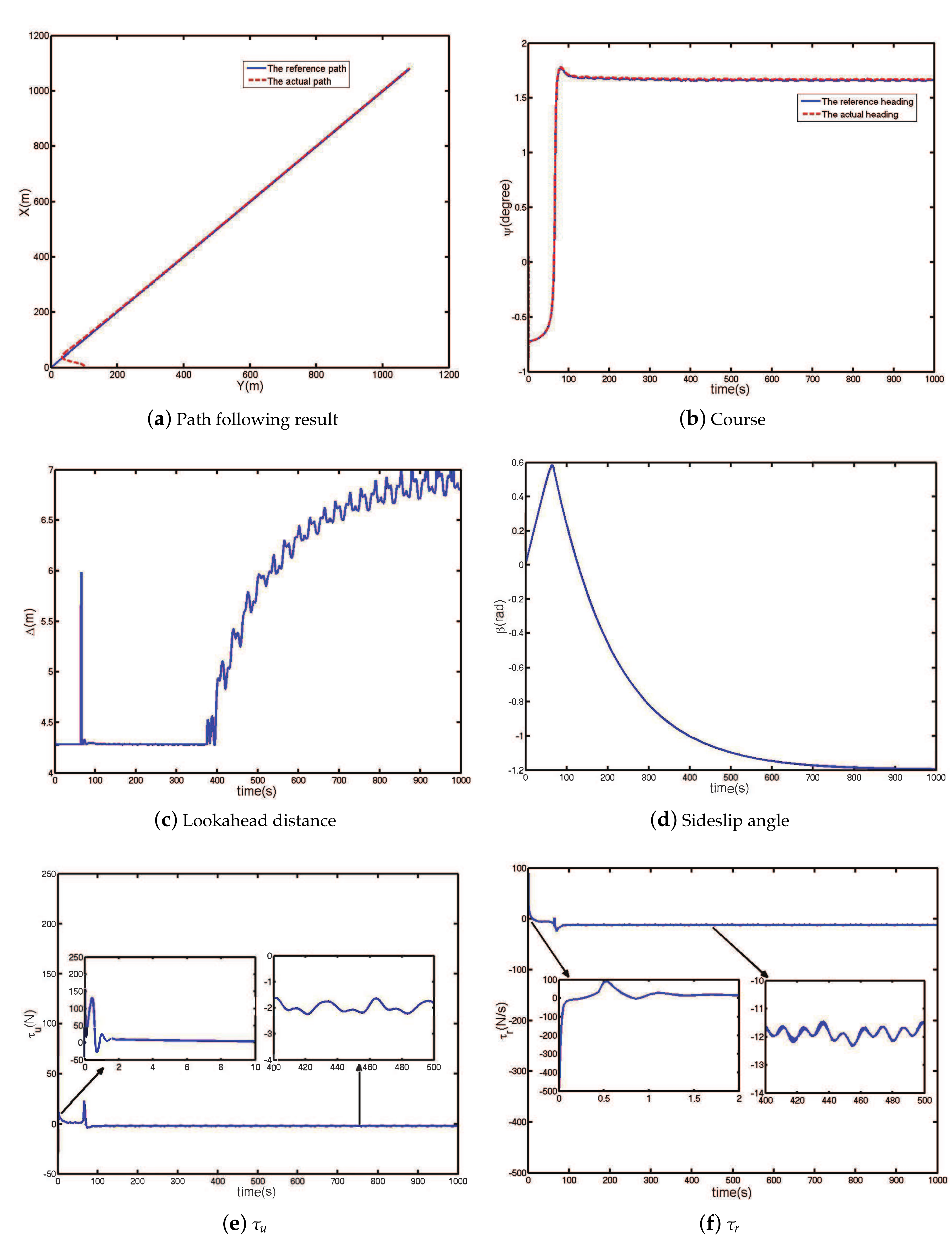
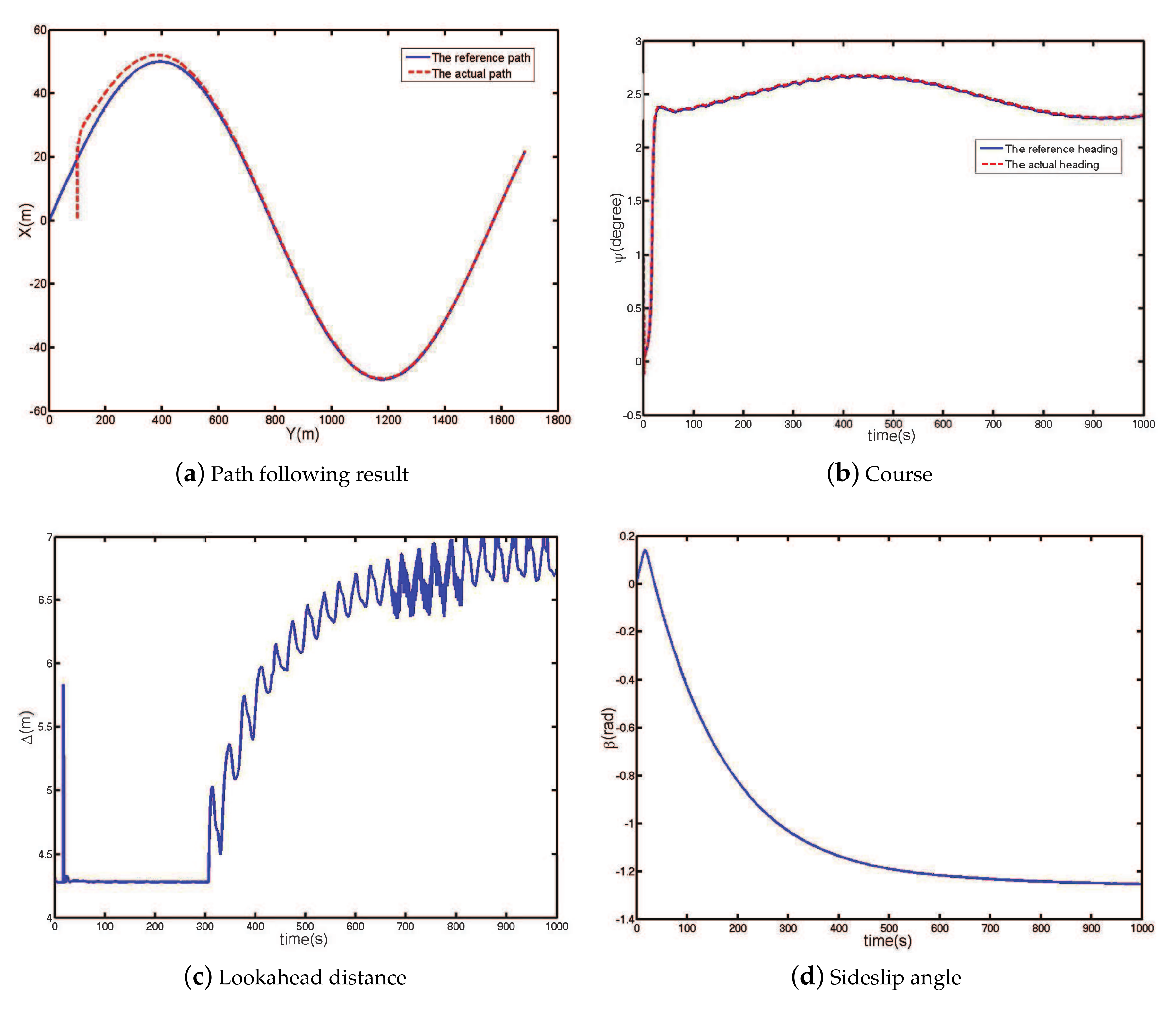
The simulation results of straight-line path following are plotted in Figure 4.

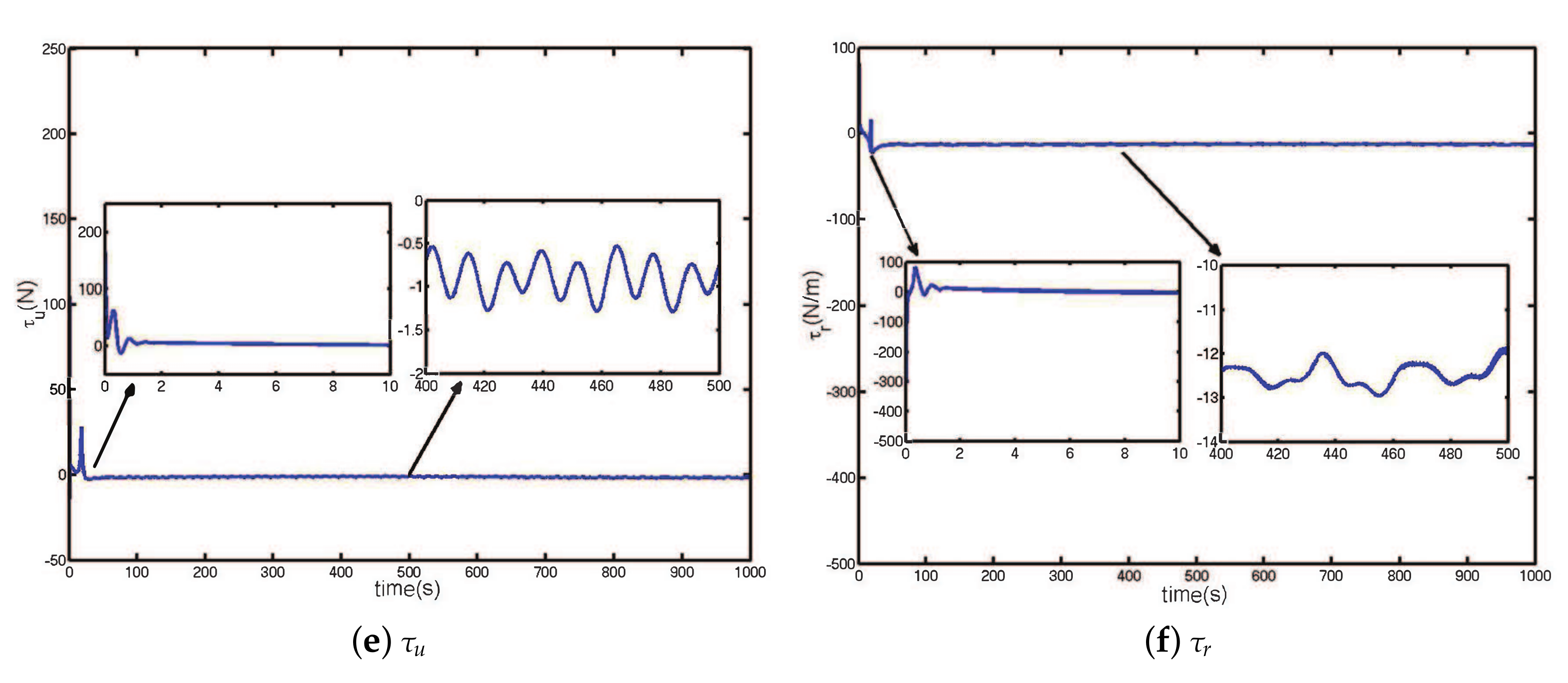
Figure 4a shows that the USV tracks the reference straight-line path accurately, which would be impossible without sideslip angle compensation. Meanwhile, it is observed that the USV converges to the reference path in a short time without obvious overshoot. The reference heading generating by the guidance system and the actual heading are depicted in Figure 4b. We can see that the actual heading can perfectly track the reference heading in the early stage of control, and even if there are external disturbances, the yaw rate controller still has a good control effect. Figure 4c shows the value of $\Delta$, and the same as the expected theoretical assumption, $\Delta$ decreases as the error decreases. The reason why its value fluctuates is due to the presence of disturbances. From Figure 4d, it is observed that the estimated value of sideslip angle has a large range of variation, which eventually converges at about −1.2 rad. We can fully expect the collapse of the entire control system if the sideslip angle is not effectively compensated. The control inputs of force ${\tau }_u$ and moment ${\tau }_r$ are depicted in Figure 4e,f. In the early stage of control, they have larger initial values, which are determined by factors such as error, control gain, the algorithm itself, and so on. If both error and control gain increase, ${\tau }_u$ and ${\tau }_r$ may produce a value greater than the actuator output capability. Therefore, it is necessary to consider the actuator saturation in the design of the controller. Besides, it is observed that they converge to an ideal range in a very short time, and certain fluctuations exist to compensate for external disturbances.

6.2. Curve Path Following

Under the condition that the guidance parameters, the control parameters, the external disturbances and the initial state of USV remain the same, the curve path following simulation is carried out. The desired geometrical path is a curve expressed as $p_d(\theta )={[50sin(\theta /\phantom{\theta 250}250),\theta ]}^T$. The simulation results of curve path following are plotted in Figure 5.

Figure 5a plots that the task of path following can still be implemented well without any navigation and control parameters unchanged, which shows that the proposed path following strategy has good adaptability. The heading tracking effect is shown in Figure 5b, and it still can maintain good control performance. The change curve of $\Delta$ is similar to that of straight-line path following, which is depicted in Figure 5c. Figure 5d displays the estimated value of sideslip angle. Similarly, the control inputs ${\tau }_u$ and ${\tau }_r$ are depicted in Figure 5e,f, respectively. They vary within a reasonable range, and ${\tau }_r$ has an input saturation phenomenon.

Thus far, the numerical simulations of straight-line path following and curve path following have achieved good results, indicating the correctness and effectiveness of the adaptive LOS navigation strategy and control strategy proposed in this paper.

6.3. Control Parameter Setting Strategy

In this subsection, some setting strategies are presented for the adjustment of the path following system parameters. The navigation module’s parameters $\kappa$, $\gamma$, ${\Delta }_{min}$ and ${\Delta }_{max}$ and the control module’s parameters $k_1$, $k_{ue}$, $k_{re}$, ${\gamma }_u$, ${\kappa }_u$, ${\gamma }_r$, ${\kappa }_r$, $K_{eu}$, ${\xi }_u$, $K_{er}$, ${\xi }_r$, A, B and D should be carefully tuned to optimize control performance. On the whole, there is no fixed principle for the adjustment of all parameters. However, according to the design principle of the path-tracking strategy and the practical experience of scholars, we can qualitatively sum up some rules.

(1)

For the navigation system, larger values of gain $\gamma$ and adaptive gain $\kappa$ mean that the sideslip angle can converge at a faster rate. Meanwhile, ${\Delta }_{min}$ and ${\Delta }_{max}$ can also affect the convergence rate. A fast convergence rate means that the sideslip angle can be compensated better, but it certainly adds to the possibility of oscillation or divergence in the navigation system.

(2)

Larger gains $k_{ue}$ and $k_{re}$ do not affect the amplitude of generated control signals in (41) and (47). They are adjusted to get the desired following performance without consideration of the actuator saturation. Nevertheless, larger $k_{ue}$ and $k_{re}$ may cause unnecessary chattering of the control signals.

(3)

Large values of adaptive gains ${\gamma }_r$ and ${\gamma }_u$ in (44) and (50) increase the learning speed of the neural network minimum parameter learning method. This means that USV can obtain more accurate following performance. However, too fast a learning speed will affect the stability of the control system. ${\kappa }_r$ and ${\kappa }_u$ are used to optimize (44) and (50), respectively.

(4)

$k_1$, A, B and D can affect the response speed of the control system. Faster system response enables USV to reach the reference path in a shorter time, but it also raises the possibility of system instability.

(5)

$K_{er}$, ${\xi }_r$, $K_{eu}$ and ${\xi }_u$ are employed to adjust the auxiliary dynamic system. Only a suitable set of parameters can be used to achieve the desired results.

In summary, the various models of the path-following system interact with each other. When adjusting the navigation or control parameters, both the control effect and the stability of the system need to be taken into consideration. Enough patience and full consideration are needed to solve this problem.

7. Conclusions

In this note, a complete set of strategies for podded propulsion USV path following is presented. First, the podded propulsion USV is proven to be an underactuated system. Then, an ALOS navigation law with a varying $\Delta$ is developed to optimize the traditional guidance scheme. In the third step, an underactuated path-following controller is proposed subject to the uncertainty of model and input saturation. The neural network minimum parameter learning method is employed to estimate the uncertain functions and external disturbances, and the neural shunting model is used to deal with the “explosion of complexity” issue. The stability of the closed-loop system is proven by Lyapunov functions. Finally, two numerical simulations demonstrate the correctness of the proposed path-following strategy.

Although this article takes into account as many practical conditions as possible, there are still problems that need to be addressed. For example, the dynamic characteristics of the thruster are not taken into consideration. In other words, the final control inputs are force (${\tau }_u$) and moment (${\tau }_r$), not propulsion angle and the rotating speed of the propeller that the pod can provide. The problem will be solved in future works.

References

- Sinisterra, A.J.; Dhanak, M.R.; Ellenrieder, K.V. Stereovision-based target tracking system for USV operations. Ocean Eng. 2017, 133, 197–214. [Google Scholar] [CrossRef]
- Yao, W.; Zhang, J.; Liu, Y.; Zhou, M.; Sun, M. Improved Vector Control for Marine Podded Propulsion Control System Based on Wavelet Analysis. J. Coast. Res. 2015, 73, 54–58. [Google Scholar] [CrossRef]
- Gierusz, W. Simulation model of the LNG carrier with podded propulsion Part 1: Forces generated by pods. Ocean Eng. 2015, 108, 105–114. [Google Scholar] [CrossRef]
- Breivik, M. Topics in Guided Motion Control of Marine Vehicles. Ph.D. Thesis, NTNU, Trondheim, Norwegian, 2010. [Google Scholar]
- Wiig, M.S.; Pettersen, K.Y.; Krogstad, T.R. Uniform semiglobal exponential stability of integral line-of-sight guidance laws. IFAC-PapersOnLine 2015, 48, 61–68. [Google Scholar] [CrossRef] [Green Version]
- Lee, S.D.; Yu, C.H.; Hsiu, K.Y.; Hsieh, Y.G.; Tzeng, C.Y. Uniform semiglobal exponential stability of integral line-of-sight guidance laws. Ocean Eng. 2010, 37, 208–217. [Google Scholar] [CrossRef]
- Hac, A.; Simpson, M.D. Estimation of vehicle side slip angle and yaw rate. SAE Trans. 2000, 109, 1032–1038. [Google Scholar]
- Borhaug, E.; Pavlov, A.; Pettersen, K.Y. Integral los control for path following of underactuated marine surface vessels in the presence of constant ocean currents. In Proceedings of the 47th IEEE Conference on Decision and Control, Cancun, Mexico, 9–11 December 2008; pp. 4984–4991. [Google Scholar]
- Lekkas, A.M.; Fossen, T.I. Integral LOS Path Following for Curved Paths Based on a Monotone Cubic Hermite Spline Parametrization. IEEE Trans. Control Syst. Technol. 2014, 22, 2287–2301. [Google Scholar] [CrossRef]
- Fossen, T.I.; Pettersen, K.Y.; Galeazzi, R. Line-of-Sight Path Following for Dubins Paths with Adaptive Sideslip Compensation of Drift Forces. IEEE Trans. Control Syst. Technol. 2015, 23, 820–827. [Google Scholar] [CrossRef]
- Lu, L.; Wang, D.; Peng, Z.; Wang, H. Stereovision-based target tracking system for USV operations. Ocean Eng. 2016, 124, 340–348. [Google Scholar]
- Pavlov, A.; Nordahl, H.; Breivik, M. MPC-Based Optimal Path Following for Underactuated Vessels. IFAC Proc. 2009, 42, 340–345. [Google Scholar] [CrossRef]
- Lekkas, A.; Fossen, T.I. A Time-Varying Lookahead Distance Guidance Law for Path Following. IFAC Proc. 2012, 45, 398–403. [Google Scholar] [CrossRef]
- Lu, L.; Wang, D.; Peng, Z. Predictor-based line-of-sight guidance law for path following of underactuated marine surface vessels. In Proceedings of the 2015 Sixth IEEE International Conference on Intelligent Control and Information Processing (ICICIP), Wuhan, China, 26–28 November 2015; pp. 284–288. [Google Scholar]
- Garus, J.; Zak, B. Using of soft computing techniques to control of underwater robot. In Proceedings of the 2010 15th IEEE International Conference on Methods and Models in Automation and Robotics (MMAR), Miedzyzdroje, Poland, 23–26 August 2010; pp. 415–419. [Google Scholar]
- Meng, W.; Guo, C.; Liu, Y.; Yang, Y.; Lei, Z. Global sliding mode based adaptive neural network path following control for underactuated surface vessels with uncertain dynamics. In Proceedings of the 2012 Third IEEE International Conference on Intelligent Control and Information Processing (ICICIP), Dalian, China, 15–17 July 2012; pp. 40–45. [Google Scholar]
- Liu, L.; Wang, D.; Peng, Z. Path following of marine surface vehicles with dynamical uncertainty and time-varying ocean disturbances. Neurocomputing 2016, 173, 799–808. [Google Scholar] [CrossRef]
- Wu, D.; Chen, M.; Gong, H.; Wu, Q. Robust Backstepping Control of Wing Rock Using Disturbance Observer. Appl. Sci. 2017, 3, 219–248. [Google Scholar] [CrossRef]
- Jiang, G.; Luo, M.; Bai, K.; Chen, S. A Precise Positioning Method for a Puncture Robot Based on a PSO-Optimized BP Neural Network Algorithm. Appl. Sci. 2017, 10, 969–982. [Google Scholar]
- Tong, S.; Li, Y.; Sui, S. Adaptive Fuzzy Output Feedback Control for Switched Nonstrict-Feedback Nonlinear Systems with Input Nonlinearities. IEEE Trans. Fuzzy Syst. 2016, 24, 1426–1440. [Google Scholar] [CrossRef]
- Chao, C.; Sutarna, N.; Chiou, J.; Wang, C. Equivalence between Fuzzy PID Controllers and Conventional PID Controllers. Appl. Sci. 2017, 6, 513–525. [Google Scholar] [CrossRef]
- Wang, H.; Wang, D.; Peng, Z. Neural network based adaptive dynamic surface control for cooperative path following of marine surface vehicles via state and output feedback. Neurocomputing 2014, 133, 170–178. [Google Scholar] [CrossRef]
- Chen, M.; Ge, S.S.; Ren, B. Adaptive tracking control of uncertain MIMO nonlinear systems with input constraints. Automatica 2011, 47, 452–465. [Google Scholar] [CrossRef]
- Du, J.; Hu, X.; Krstić, M.; Sun, Y. Robust dynamic positioning of ships with disturbances under input saturation. Automatica 2016, 73, 207–214. [Google Scholar] [CrossRef]
- Wang, H.; Wang, D.; Peng, Z. Adaptive dynamic surface control for cooperative path following of marine surface vehicles with input saturation. Nonlinear Dyn. 2014, 77, 107–117. [Google Scholar] [CrossRef]
- Fossen, T.I. Marine Control Systems: Guidance, Navigation and Control of Ships, Rigs and Underwater Vehicles. In Marine Cybernetics; Springer: Trondheim, Norway, 2002. [Google Scholar]
- Zhang, G.; Zhang, X. A novel DVS guidance principle and robust adaptive path-following control for underactuated ships using low frequency gain-learning. Isa Trans. 2015, 56, 75–85. [Google Scholar] [CrossRef] [PubMed]
- Li, J.H.; Lee, P.M.; Jun, B.H.; Lin, Y.K. Point-to-point navigation of underactuated ships. Automatica 2008, 44, 3201–3205. [Google Scholar] [CrossRef]
- Ge, S.S.; Wang, C. Direct adaptive NN control of a class of nonlinear systems. IEEE Trans. Neural Netw. 2002, 13, 214–221. [Google Scholar] [CrossRef] [PubMed]
- Chen, B.; Liu, X.; Liu, K.; Lin, C. Direct adaptive fuzzy control of nonlinear strict-feedback systems. Automatica 2009, 45, 1530–1535. [Google Scholar] [CrossRef]
- Yang, Y.; Du, J.; Liu, H.; Abraham, A. A Trajectory Tracking Robust Controller of Surface Vessels with Disturbance Uncertainties. IEEE Trans. Control Syst. Technol. 2014, 22, 1511–1518. [Google Scholar] [CrossRef]
- Dai, S.L.; Wang, C.; Luo, F. Identification and Learning Control of Ocean Surface Ship Using Neural Networks. IEEE Trans. Ind. Inform. 2012, 8, 801–810. [Google Scholar] [CrossRef]
- Pan, C.Z.; Lai, X.Z.; Yang, S.X.; Wu, M. An efficient neural network approach to tracking control of an autonomous surface vehicle with unknown dynamics. Expert Syst. Appl. 2013, 40, 1629–1635. [Google Scholar] [CrossRef]
Figure 1.
The Earth-fixed inertial and body-fixed frame.
Figure 2.
LOS guidance geometry for curved paths.
Figure 3.
The block diagram of the podded propulsion USV path following.
Figure 4.
The results of the straight-line path following.
Figure 5.
The results of the curve path following.
© 2017 by the authors. Licensee MDPI, Basel, Switzerland. This article is an open access article distributed under the terms and conditions of the Creative Commons Attribution (CC BY) license (http://creativecommons.org/licenses/by/4.0/).
Share and Cite
MDPI and ACS Style
Mu, D.; Wang, G.; Fan, Y.; Sun, X.; Qiu, B. Adaptive LOS Path Following for a Podded Propulsion Unmanned Surface Vehicle with Uncertainty of Model and Actuator Saturation. Appl. Sci. 2017, 7, 1232. https://doi.org/10.3390/app7121232
AMA Style
Mu D, Wang G, Fan Y, Sun X, Qiu B. Adaptive LOS Path Following for a Podded Propulsion Unmanned Surface Vehicle with Uncertainty of Model and Actuator Saturation. Applied Sciences. 2017; 7(12):1232. https://doi.org/10.3390/app7121232
Chicago/Turabian StyleMu, Dongdong, Guofeng Wang, Yunsheng Fan, Xiaojie Sun, and Bingbing Qiu. 2017. "Adaptive LOS Path Following for a Podded Propulsion Unmanned Surface Vehicle with Uncertainty of Model and Actuator Saturation" Applied Sciences 7, no. 12: 1232. https://doi.org/10.3390/app7121232
Note that from the first issue of 2016, this journal uses article numbers instead of page numbers. See further details here.