A New Online Secondary Path Modeling Method with An Auxiliary Noise Power Scheduling Strategy for Narrowband Active Noise Control Systems

Department of Automatic Testing and Control, Harbin Institute of Technology, Harbin 150080, China
*
Authors to whom correspondence should be addressed.
Appl. Sci. 2017, 7(12), 1236; https://doi.org/10.3390/app7121236
Submission received: 10 October 2017
/
Revised: 9 November 2017
/
Accepted: 27 November 2017
/
Published: 29 November 2017
(This article belongs to the Section Acoustics and Vibrations)
Abstract
:In recent years, the online secondary path modeling (SPM) method with an auxiliary noise power scheduling strategy has been crucial for active noise control (ANC) systems and has also become a popular research topic. However, most scheduling strategies have been designed for broadband active noise control (BANC), and these ideas may not be directly applied to narrowband active noise control (NANC) systems due to the difference in structure between BANC and NANC systems. In this paper, a new online SPM method with auxiliary noise power scheduling is proposed. Here, the controlled system is adapted using the filtered-x weighted accumulated least mean square (FXWALMS) algorithm proposed by the authors. Moreover, the auxiliary noise power is scheduled based on the convergence status of the forgetting factor to accurately track the change in the NANC system. As a result, the proposed method not only achieves good modeling accuracy and fast convergence but also considerably increases noise attenuation. Extensive simulations are conducted to prove the superior performance of the proposed method in various scenarios.
1. Introduction
In the past few years, the research on active noise control (ANC) technology has received considerable attention as more and more applications have appeared [1,2,3,4,5], and several systems and algorithms have been proposed by various researchers [6,7,8,9,10,11,12]. The ANC technique can be used to effectively attenuate low-frequency acoustic noises for which the passive noise control (PNC) techniques [13] are either ineffective or increase the bulk and cost of entire systems. The main theory behind ANC is based on the superposition principle of acoustic waves, where an antinoise of equal amplitude and opposite phase is generated and combined with the primary noise by an ANC system, resulting in the cancellation of both noises. With the widespread use of industrial equipment, various annoying noise signals are generated by rotating machines, such as fans, compressors, and engines. These types of noises include multiple narrowband components, exhibit narrowband characteristics, and usually can be modeled as multiple sinusoidal signals with additive white noise. The narrowband active noise control (NANC) system can suppress such noise signals more efficiently in various engineering and environmental applications.
The modeling issue of the secondary path plays crucial role in stabilizing the ANC system. The model of the secondary path can be obtained using an offline modeling technique before the operation of ANC system. However, for a practical ANC application, a primary noise signal always exists, and the acoustics transfer function of the secondary path may be time-varying. Under these situations, online secondary path modeling (SPM) is essential for ensuring the stability of the ANC system.
Several contributions to the research on online SPM methods have been made by many researchers. The use of auxiliary noise power injection with fixed power was originally proposed by Eriksson [14]. The original idea of Eriksson’s method was later modified and extended in [15,16,17,18,19], which used fixed power auxiliary noise in all operating situations. Nevertheless, the fixed power auxiliary noise contributes to the residual error, which we want to minimize, and leads to the performance degradation of the ANC system in the steady state. To remedy this problem, various auxiliary noise power scheduling strategies have been proposed [20,21,22,23,24,25]. However, it should be noted that most of the above mentioned strategies were designed for broadband active noise control (BANC). These strategies cannot be directly applied to an NANC system because the primary noise signal, which is used in the strategies and can be obtained for a BANC system, cannot be obtained for an NANC system. The detailed performance analysis of the NANC system with online SPM using Eriksson’s method was provided by Xiao [26]. In [27], the method of scaling auxiliary noise by one-delayed residual noise signal was proposed for NANC system equipped with an online SPM subsystem and the detailed performance analysis is also given.
In this study, we are mainly concerned with NANC with an online SPM system and propose a new online SPM method with an auxiliary noise power scheduling strategy. The method we proposed is a further extension of previous works by the authors of [12,28]. First, a variable forgetting factor filtered-x weighted accumulated least mean square (FXWALMS) algorithm [28] is introduced into the control filter in order to improve the convergence and tracking performance of the system. Second, according to the range of the forgetting factor, the new auxiliary noise power is scheduled based on the convergence status of the forgetting factor to accurately track the change in the NANC system. As a result, the proposed method not only achieves better modeling accuracy but also considerably reduces the residual noise. Extensive simulations are conducted to demonstrate that the proposed system can improve the overall performance of the system effectively.
The rest of the paper is organized as follows. In Section 2, the existing online SPM method for NANC systems is briefly introduced. Section 3 presents the proposed method in detail. In Section 4, simulation results are given to verify the effectiveness of the proposed method under various scenarios. Finally, conclusions are given in Section 5.
2. Existing Online Secondary Path Modeling (SPM) Method for Narrowband Active Noise Control (NANC) Systems
2.1. Basic NANC System with Online SPM
By applying Eriksson’s method [14] to an NANC system, Xiao [26] introduced and analyzed a basic NANC system with online SPM. The block diagram of the NANC system equipped with auxiliary white noise is shown in Figure 1. The whole system is composed of two subsystems. One, called the NANC subsystem, synthesizes the secondary source signal, for which a linear combiner (LC) is used as the controller and an adaptive notch filter is used as a noise canceler to mitigate the primary noise . The other, called the SPM subsystem, estimates the secondary path, for which fixed-power auxiliary noise is used as the training signal.
The primary noise can be represented as
where q is the number of frequency components of the primary noise, is the frequency of the ith component, and is a zero-mean additive white noise with variance . are the discrete Fourier coefficients (DFC) of the ith frequency components. The reference sine and cosine waves, which are generated by a synchronization signal from a nonacoustic sensor, such as a tachometer [29], are defined as
where is identified from the synchronization signal. The output of the secondary source signal generated by the NANC subsystem is expressed as
where are DFC estimations of the secondary source, updated using some adaptive algorithms. The true secondary path is modeled by a moving average (MA) system
where M is the model order and are the model coefficients. The error signal is measured using an error microphone, given by
where
where is the auxiliary white Gaussian noise with zero mean and variance .
In the NANC subsystem, the FXLMS algorithm is used to update the DFC estimation of the secondary source, given by
where is the step size, which directly determines the convergence speed, and and are the input filtered reference signals, which can be calculated using
where is the estimate of the secondary path, which is identified and utilized simultaneously by the SPM subsystem while the whole system is in operation. Parameters and are the order and finite pulse response (FIR) coefficients of the secondary path estimate , respectively.
In the SPM subsystem, is the training signal of the subsystem. The coefficient (weight) vector of the filter and the input reference signal vector are defined, respectively, as follows
The output of the filter is given by
where * denotes linear convolution. The corresponding error signal is calculated using
The LMS algorithm used to update the coefficient vector of the SPM subsystem given as
where is the step size, which directly determines the convergence speed of the SPM subsystem.
2.2. NANC System with Online SPM Using Scaled Auxiliary Noise Injection
The fixed power auxiliary noise used in Figure 1 contributes to the residual error and causes the low convergence speed of the system. To address this problem, a NANC system equipped with an online SPM subsystem that uses auxiliary noise scaled by one-delayed residual noise signal was proposed in [27], the block diagram of which is depicted in Figure 2. We see that this structure is similar to that of Xiao’s method shown in Figure 1, except for the addition of an auxiliary noise power scheduling strategy called noise power scheduling.
The auxiliary noise power scheduled based on the status of the one-sample-delayed residual noise signal can be expressed as
The signal can be recalculated as
Substituting the above equation into Equation (5), one has
The FXLMS algorithm for DFC estimation and the LMS algorithm for the coefficient vector of are expressed as
From Equations (18), (20), and (22), the auxiliary noise is scaled by an absolute value of the one-sample-delayed residual noise signal. Then, it is added with the output of the NANC subsystem and acts as a secondary source. Meanwhile, it is also entered into the secondary path model. When the system is close to the steady state, the scaled auxiliary noise becomes very small, significantly reducing the residual noise signal of the overall system.
3. Proposed Method
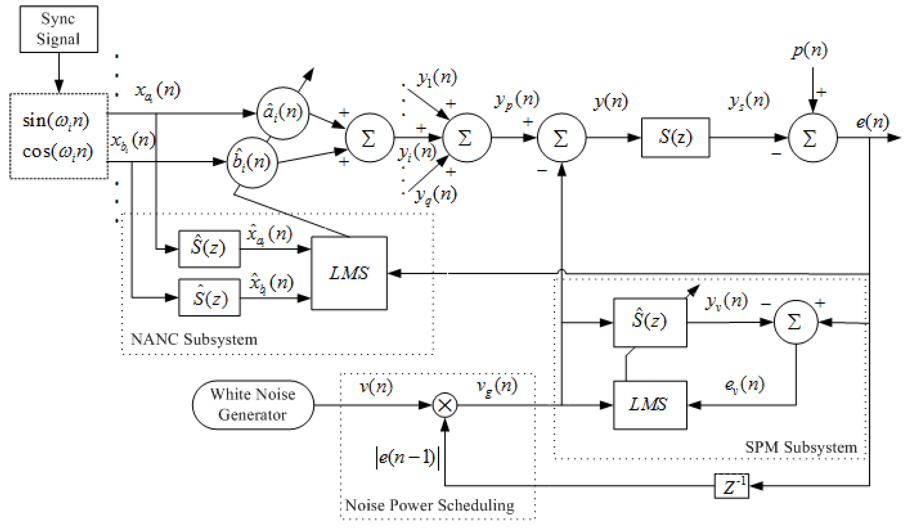
Here, a new online SPM method with an auxiliary noise power scheduling strategy for the NANC system is proposed by extending the method developed by the authors [28] to improve the performance of the whole system. The block diagram of the proposed method is shown in Figure 3. We see that the structure of the proposed method is similar to that of Liu’s method shown in Figure 2, except for some modifications in the following subsystem.
First, let us consider the NANC subsystem shown in Figure 3. To increase the convergence rate and traceability, a modified FXWALMS (MFXWALMS) algorithm with the variable forgetting factor scheme [28] is used in the NANC subsystem. The MFXWALMS algorithm for the DFC estimates of the secondary source can be rewritten as
where is the time-varying forgetting factor, the update equation of which can be expressed as
In the above equation, and are similar to those used in the algorithm of [28]. The upper limit parameter can be used to avoid values that are too large and to make the system more stable. Here, we substitute the error autocorrelation of the entire system for the error autocorrelation of the NANC subsystem to update , as is used in the two subsystems and the residual error of the entire system can better indicate the status of the whole system compared to the error signal of the NANC subsystem.
For the online SPM subsystem, according to the characteristics of the range of the variable forgetting factor , new auxiliary noise power scheduled based on the convergence status of can be expressed as
Similarly, the signal can be recalculated as
Substituting the above equation into Equation (5), one has
The LMS algorithm for the coefficient vector of is given by
Using error autocorrelation to update not only is a good measure of the proximity to the optimum but also can reduce the effect of the uncorrelated noise. Generally, the error autocorrelation estimate is a large value in the convergence stages or error bursting, which may be caused by the changes in the secondary path or primary noise, resulting in a large . When the adaptation process approaches the steady state, the value of the error autocorrelation approaches zero, resulting in a small . These characteristics of the change in are very useful for the two subsystems. For the NANC subsystem, the large improves the convergence speed and tracing capabilities, and the small can ensure a low misadjustment. For the SPM subsystem, the auxiliary noise is scaled by before it is added to the entire system. In this way, the large will yield a large , which can improve modeling accuracy. Moreover, the power of the auxiliary noise scaled by will become very small, which can significantly reduce the of the system when the adaptive process approaches the steady state.
4. Simulations and Results
Extensive simulations are performed to demonstrate the effectiveness of the proposed method under different scenarios. The simulation performance of the proposed method is compared with that of existing methods, referred to herein as Method 1 [26] and Method 2 [27]. The comparison of the overall system performances is carried out based on the following performance measures:
- Relative modeling error of the secondary path, defined as
- Mean square error (MSE) at the error microphone, .
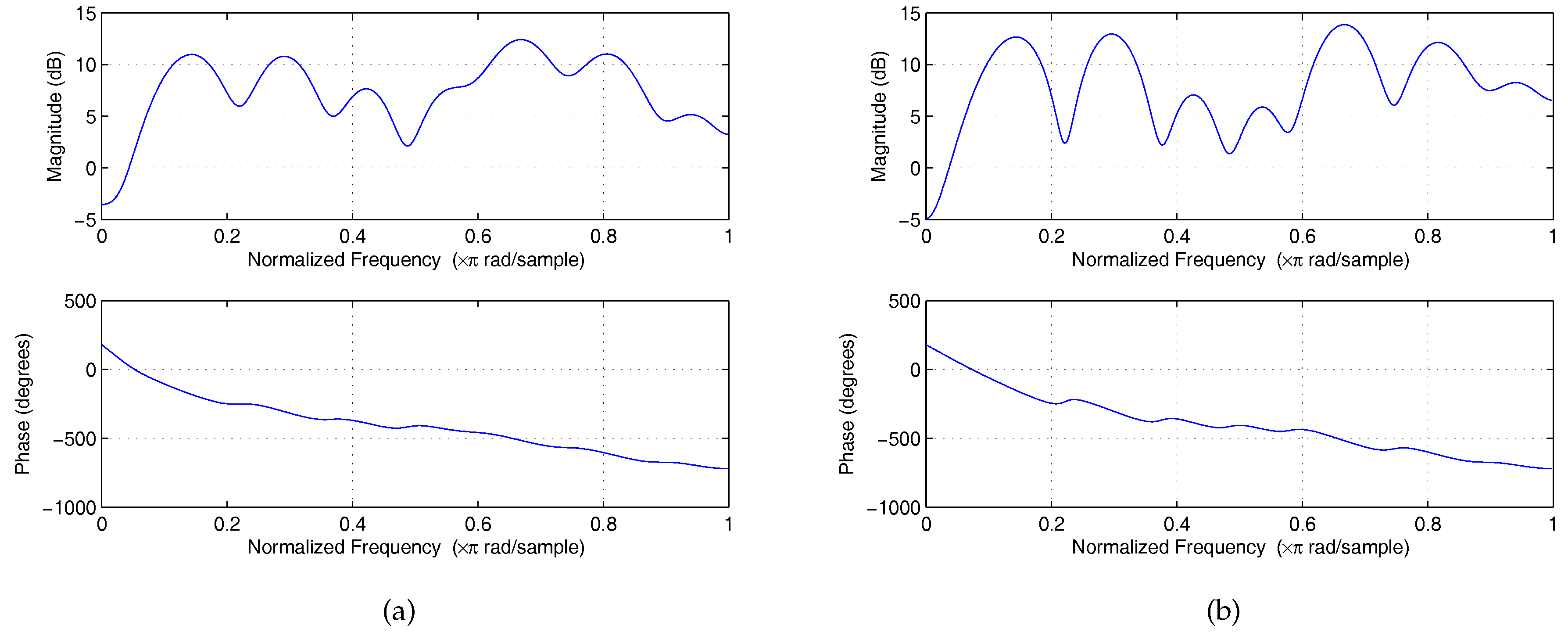
The secondary path adopts a truncated impulse response of the acoustic path, which is an experimental datapoint provided in [29]. and its estimates are FIR filters of the order . The frequency responses of are shown in Figure 4. A zero-mean white Gaussian noise with variance is used as a training signal in the SPM, and a scaled factor k is used to initialize the power of the for different methods to obtain better performances in the simulations. Moreover, a zero-mean white Gaussian noise of variance is added to the primary noise as a measurement noise . For each of the simulation results, a Monte Carlo average over 100 has been achieved. The main simulation results are given as follows.
4.1. Case 1
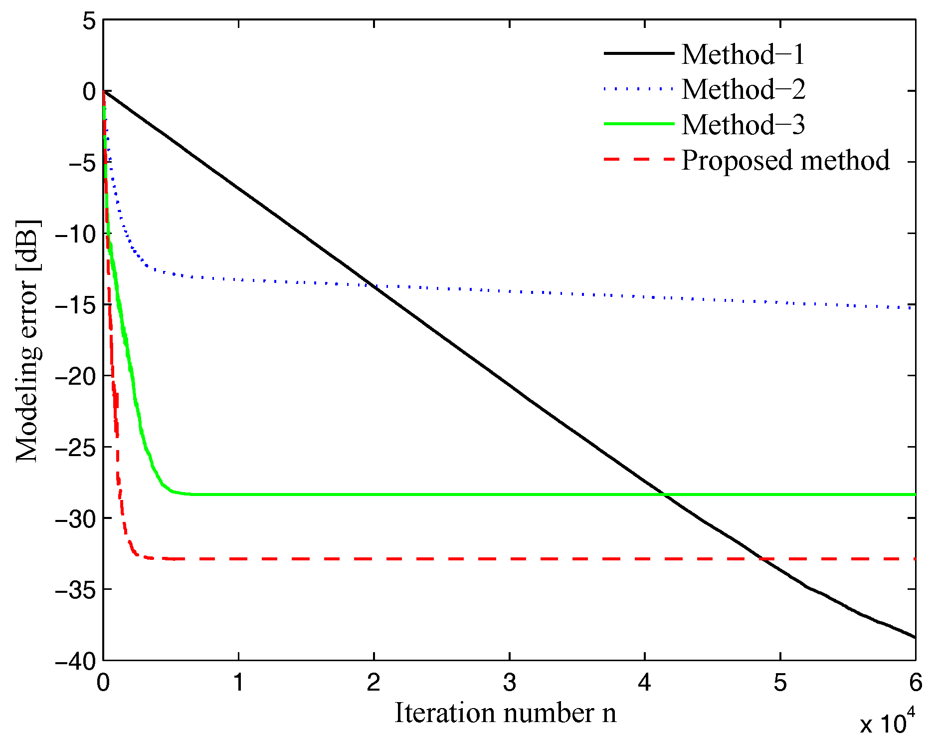
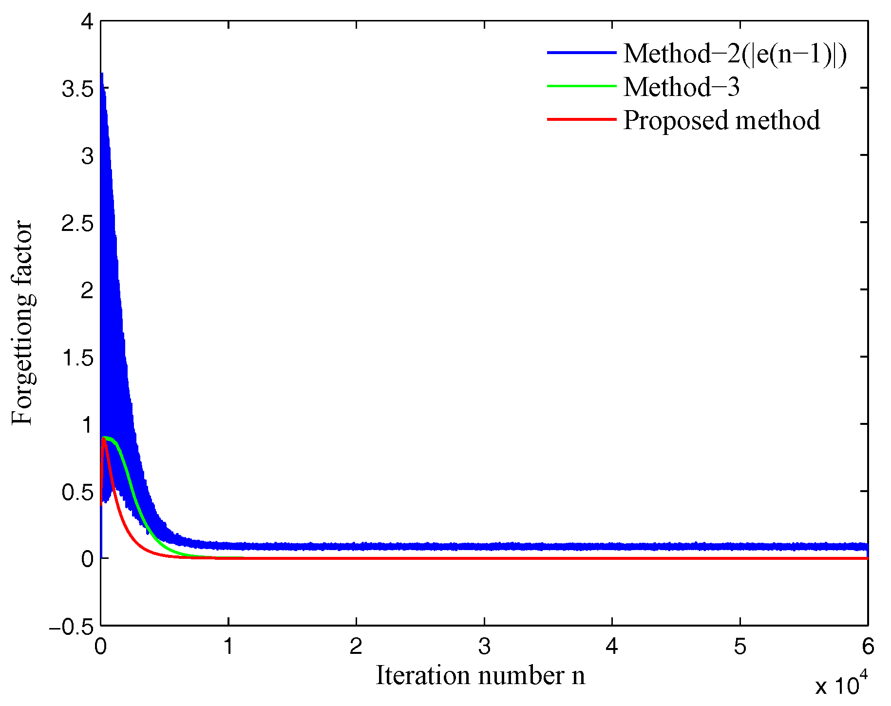
In this case, the primary noise includes three frequencies : , , and . The corresponding DFCs are set to , , , , and , , respectively. is the fixed secondary path. The frequency responses of are shown in Figure 4a. To compare the scaling strategy of and more clearly, Method 3, which uses auxiliary noise scheduled based on but employs the same NANC subsystem as that of Method 2, is included in the comparison. The parameters of the four methods are set as follows. In Method 1, for all i, , and the scaled factor . The corresponding parameters in Method 2 are for all i, , and . The parameters used in Method 3 and the proposed method are for all i, , , , , and , and the initial forgetting factor is set as . The simulation results for Case 1 are provided in Figure 5, Figure 6, Figure 7 and Figure 8.
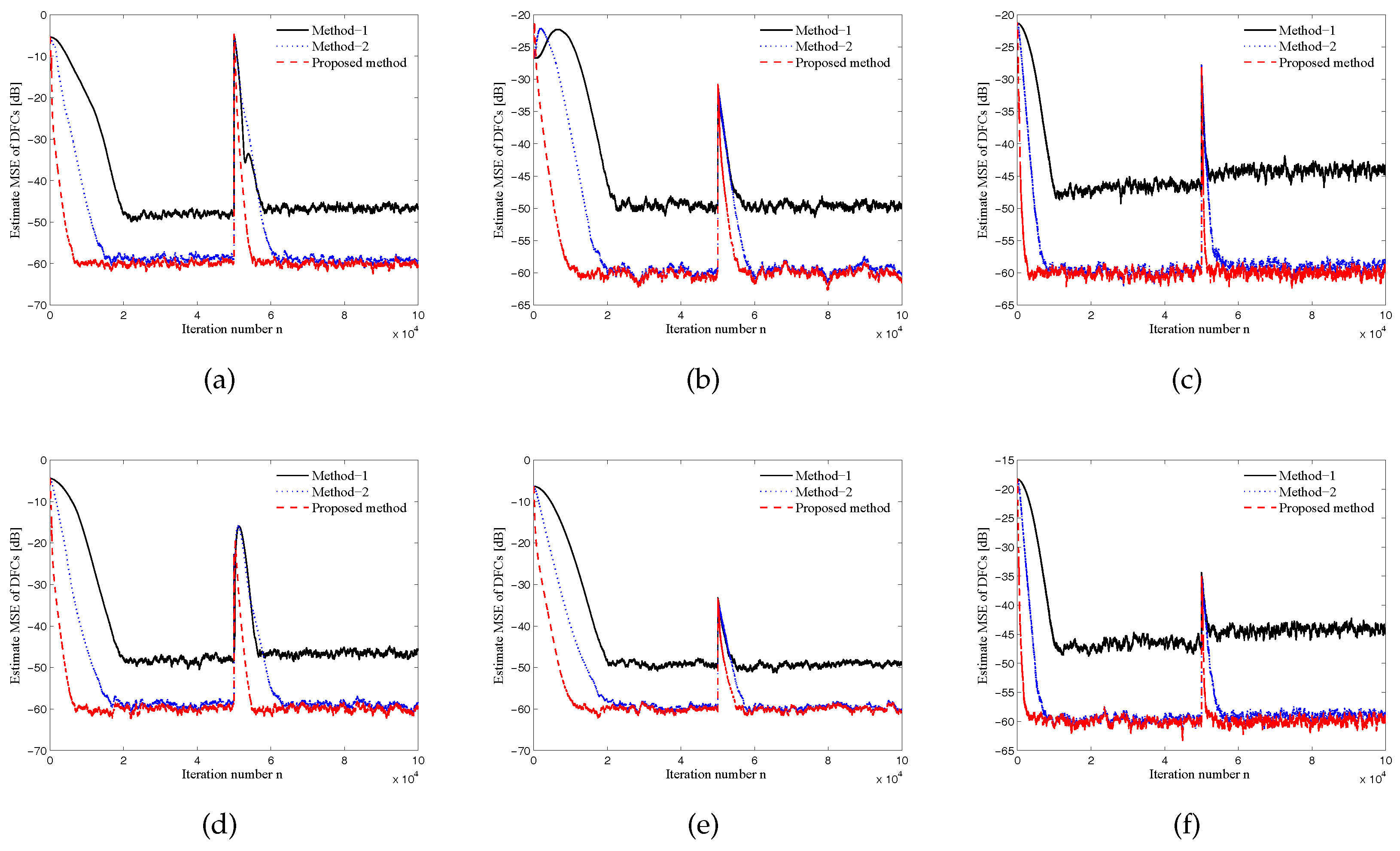
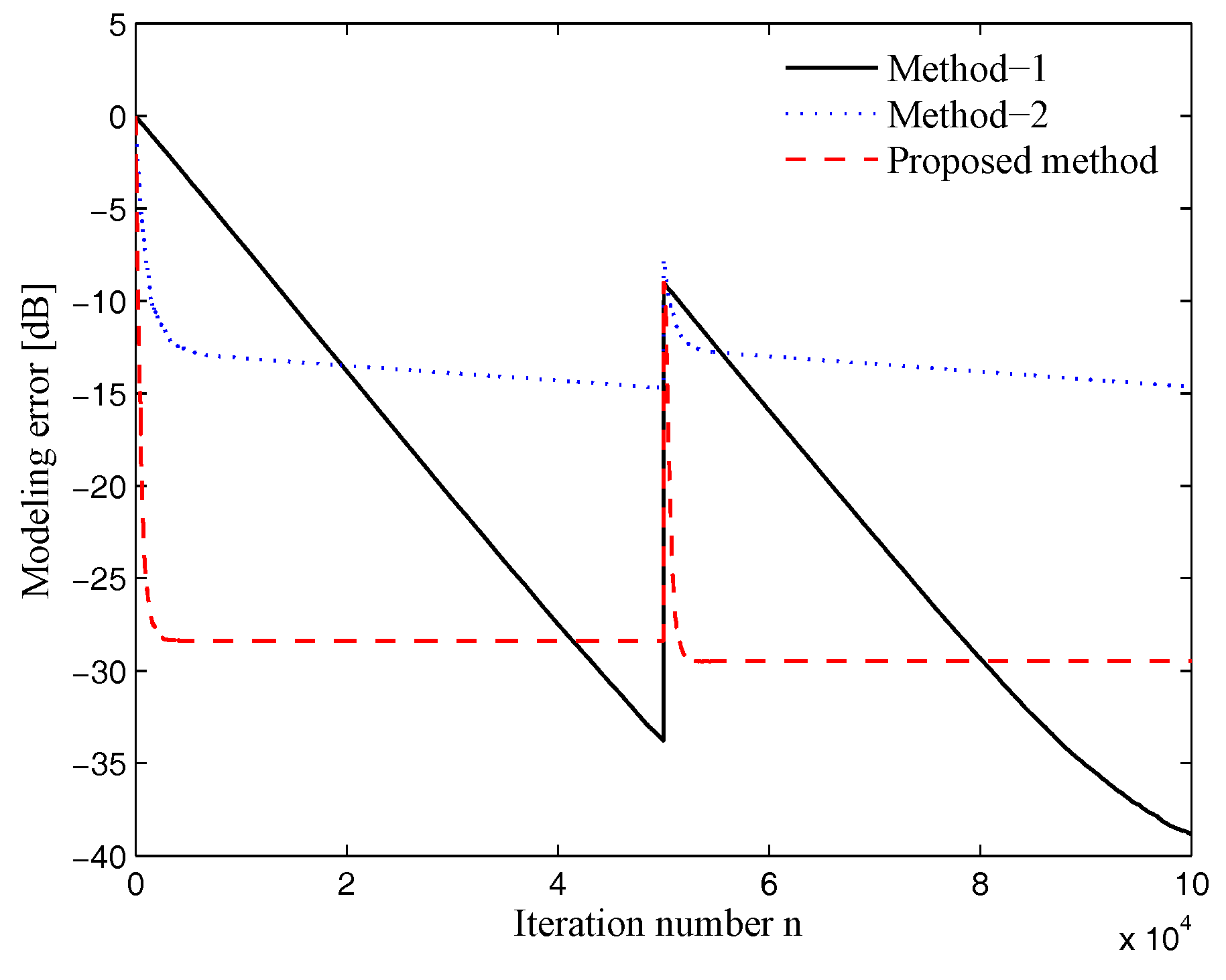
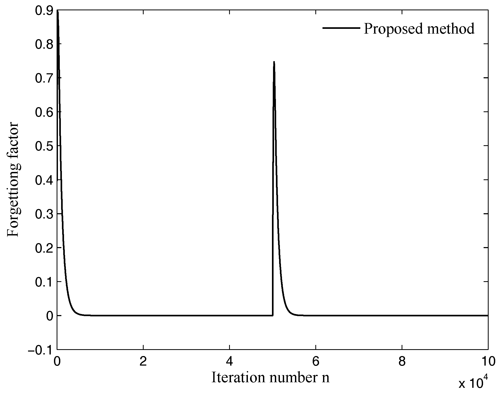
Figure 5a–f shows comparisons between the DFC estimation MSEs of Method 1, Method 2, Method 3, and the proposed method. The MSEs are displayed in Figure 6a. To identify the system performance more clearly, each MSE value for the plot was obtained by averaging the square values of 50 past residue errors, as shown in Figure 6b. The modeling error and the mean variable forgetting factor of the proposed method are shown in Figure 7 and Figure 8, respectively. To show the process of adjusting the auxiliary noise carried out in Method 2, the of Method 2 is shown in Figure 8.
The following remarks can be made based on above simulation results.
(1) Regarding the performance of convergence, the proposed method has a faster rate of convergence, as a result of using the FXWALMS algorithm, than that of Method 1 and Method 2, as shown in Figure 5a–f and Figure 6.
(2) Regarding the steady-state performance of the system, the fixed power auxiliary noise used in Method 1 not only contributes to the residual error but also seriously degrades the steady-state performance of the DFC estimation MSEs. However, the proposed method and Method 2 have better steady-state performances than Method 1. Moreover, although Method 2 has a similar steady-state performance to that of the proposed method based on the DFC estimation MSEs, the proposed method has a better steady-state performance for the residual error , as shown in Figure 5a–f and Figure 6. The reason for the improved noise-reduction performance is that the proposed auxiliary noise power scheduling strategy results in a smaller auxiliary noise power in the steady state than that of Method 2.
(3) Compared with Method 2, the proposed method can achieve a better modeling accuracy. Although Method 1 achieves good modeling accuracy, the low convergence and poor steady-state performance seriously degrade the overall performance of the system, as indicated in Figure 7.
(4) The curves of the mean variable forgetting factor of the proposed method clearly indicate the status of convergence, as shown in Figure 8. Generally, it is better if the scaling strategy has the ability to quickly vary the auxiliary noise in the convergence stage; moreover, small auxiliary noise power is better when the algorithm is approaching the steady state. In addition, large jumps to adjust the auxiliary noise will adversely affect the convergence performance. is a time-varying forgetting factor, and its value can be computed by weighting the historical autocorrelation errors. The scaling strategy of uses only the current error information. The fluctuation of will significantly affect the convergence speed. Since the weighting of the historical autocorrelation errors plays an important role in reducing the volatility, the convergence process of the system using in the SPM subsystem can be faster and more stable.
4.2. Case 2
In this case, the same primary noise as in Case 1 is adopted in the simulation. The secondary path is suddenly changed in the middle of the adaptive process ( 50,000). The frequency responses of the original and changed path are shown in Figure 4a,b, respectively. The parameters of the three methods are set as follows. In Method 1, , for all i, and . In Method 2, for all i, , and . The parameters used in the proposed method are for all i, , , , , and the value of the forgetting factor is initially set as . Similar comparisons to those conducted for Case 1 are provided in Figure 9, Figure 10, Figure 11 and Figure 12. From these figures, we see that the proposed method can not only yield excellent performances similar to those in Case 1 but also accurately track the change in the secondary path. Therefore, the proposed method again performs well and outperforms Method 1 and Method 2 in terms of the variable secondary path.
5. Conclusions
A new online SPM method using an auxiliary noise power scheduling strategy for NANC systems was proposed and investigated in detail via extensive simulations in this paper. The proposed method uses a variable forgetting factor FXWALMS algorithm to adapt the control filter of the NANC subsystem to improve its convergence property and tracking performance. Furthermore, a new auxiliary noise power scheduling strategy was designed for the online SPM subsystem. According to the proposed scheduling method, the forgetting factor is used to adjust the auxiliary noise power for accurately tracking the convergence status of the NANC system. Consequently, the proposed method not only achieves good modeling accuracy and fast convergence but also improves the noise-reduction performance of the NANC system in the steady state. The presented simulation results also demonstrate good stability and dynamic tracking performance regarding a change in the secondary path.
Acknowledgments
The authors would like to thank the anonymous reviewers for their valuable comments, which contributed to improvements made to this paper. This work was supported by the National Science and Technology Support Program of China (No. 2012BAI34B03-3).
Author Contributions
Chao Sun and Zhong Bo conceived and designed the simulation experiments; Yuqi Liu performed the simulation experiments; Chao Sun and Shouda Jiang analyzed the data; Chao Sun and Zhong Bo wrote the paper; Yuqi Liu contributed to the revision of the article.
Conflicts of Interest
The authors declare no conflict of interest. The founding sponsors had no role in this study.
References
- Kajikawa, Y.; Gan, W.S.; Kuo, S.M. Recent advances on active noise control: Open issues and innovative applications. APSIPA Trans. Signal Inf. Process. 2012, 1, 1–21. [Google Scholar] [CrossRef]
- Liu, L.; Kuo, S.M. Wireless communication integrated active noise control system for infant incubators. In Proceedings of the 2013 IEEE International Conference on Acoustics, Speech and Signal Processing (ICASSP), Vancouver, BC, Canada, 26–31 May 2013; pp. 375–378. [Google Scholar]
- Veena, S.; Pavithra, S.; Lokesha, H.; Narasimhan, S.; More, N.V. Virtual sensor based Feedback Active Noise Control for neonates in NICU. In Proceedings of the 2013 International Conference on Emerging Trends in Communication, Control, Signal Processing & Computing Applications (C2SPCA), Bangalore, India, 10–11 October 2013; pp. 1–5. [Google Scholar]
- Miyazaki, N.; Yamakawa, K.; Kajikawa, Y. Head-mounted active noise control system to achieve speech communication. In Proceedings of the 2013 Asia-Pacific Signal and Information Processing Association Annual Summit and Conference (APSIPA), Kaohsiung, Taiwan, 29 October–1 November 2013; pp. 1–6. [Google Scholar]
- Jena, D.; Sahoo, S.; Panigrahi, S. Gear fault diagnosis using active noise cancellation and adaptive wavelet transform. Measurement 2014, 47, 356–372. [Google Scholar] [CrossRef]
- Kuo, S.M.; Kuo, K.; Gan, W.S. Active noise control: Open problems and challenges. In Proceedings of the 2010 International Conference on Green Circuits and Systems (ICGCS), Shanghai, China, 21–23 June 2010; pp. 164–169. [Google Scholar]
- Xiao, Y. A new efficient narrowband active noise control system and its performance analysis. IEEE Trans. Audio Speech Lang. Process. 2011, 19, 1865–1874. [Google Scholar] [CrossRef]
- Montazeri, A.; Poshtan, J. A new adaptive recursive RLS-based fast-array IIR filter for active noise and vibration control systems. Signal Process. 2011, 91, 98–113. [Google Scholar] [CrossRef]
- Ferrer, M.; Gonzalez, A.; de Diego, M.; Pinero, G. Convex combination filtered-x algorithms for active noise control systems. IEEE Trans. Audio Speech Lang. Process. 2013, 21, 156–167. [Google Scholar] [CrossRef]
- Li, J.Y.; Kuo, S.M.; Chang, C.Y. Splitting frequency components of error signal in narrowband active noise control system design. In Proceedings of the 2013 Asia-Pacific Signal and Information Processing Association Annual Summit and Conference (APSIPA), Kaohsiung, Taiwan, 29 October–1 November 2013; pp. 1–6. [Google Scholar]
- George, N.V.; Panda, G. Advances in active noise control: A survey, with emphasis on recent nonlinear techniques. Signal Process. 2013, 93, 363–377. [Google Scholar] [CrossRef]
- Bo, Z.; Sun, C.; Xu, Y.; Jiang, S. A variable momentum factor filtered-x weighted accumulated LMS algorithm for narrowband active noise control systems. Measurement 2014, 48, 282–291. [Google Scholar] [CrossRef]
- Harris, C.M. Handbook of Acoustical Measurements and Noise Control; McGraw-Hill: New York, NY, USA, 1991. [Google Scholar]
- Eriksson, L.; Allie, M. Use of random noise for on-line transducer modeling in an adaptive active attenuation system. J. Acoust. Soc. Am. 1989, 85, 797–802. [Google Scholar] [CrossRef]
- Bao, C.; Sas, P.; Van Brussel, H. Adaptive active control of noise in 3-D reverberant enclosures. J. Sound Vib. 1993, 161, 501–514. [Google Scholar] [CrossRef]
- Zhang, M.; Lan, H.; Ser, W. Cross-updated active noise control system with online secondary path modeling. IEEE Trans. Speech Audio Process. 2001, 9, 598–602. [Google Scholar] [CrossRef]
- Akhtar, M.T.; Abe, M.; Kawamata, M. A new variable step size LMS algorithm-based method for improved online secondary path modeling in active noise control systems. IEEE Trans. Audio Speech Lang. Process. 2006, 14, 720–726. [Google Scholar] [CrossRef]
- Davari, P.; Hassanpour, H. A self-tuning feedforward active noise control system. IEICE Electron. Express 2009, 6, 230–236. [Google Scholar] [CrossRef]
- Hassanpour, H.; Davari, P. An efficient online secondary path estimation for feedback active noise control systems. Digit. Signal Process. 2009, 19, 241–249. [Google Scholar] [CrossRef]
- Zhang, M.; Lan, H.; Ser, W. A robust online secondary path modeling method with auxiliary noise power scheduling strategy and norm constraint manipulation. IEEE Trans. Speech Audio Process. 2003, 11, 45–53. [Google Scholar] [CrossRef]
- Akhtar, M.; Abe, M.; Kawamata, M. Noise power scheduling in active noise control systems with online secondary path modeling. IEICE Electron. Express 2007, 4, 66–71. [Google Scholar] [CrossRef]
- Carini, A.; Malatini, S. Optimal variable step-size NLMS algorithms with auxiliary noise power scheduling for feedforward active noise control. IEEE Trans. Audio Speech Lang. Process. 2008, 16, 1383–1395. [Google Scholar] [CrossRef]
- Davari, P.; Hassanpour, H. Designing a new robust on-line secondary path modeling technique for feedforward active noise control systems. Signal Process. 2009, 89, 1195–1204. [Google Scholar] [CrossRef]
- Ahmed, S.; Akhtar, M.T.; Zhang, X. Robust auxiliary-noise-power scheduling in active noise control systems with online secondary path modeling. IEEE Trans. Audio Speech Lang. Process. 2013, 21, 749–761. [Google Scholar] [CrossRef]
- Aslam, M.S.; Raja, M.A.Z. A new adaptive strategy to improve online secondary path modeling in active noise control systems using fractional signal processing approach. Signal Process. 2014, 107, 433–443. [Google Scholar] [CrossRef]
- Xiao, Y.; Ma, L.; Hasegawa, K. Properties of FXLMS-based narrowband active noise control with online secondary-path modeling. IEEE Trans. Signal Process. 2009, 57, 2931–2949. [Google Scholar] [CrossRef]
- Liu, J.; Xiao, Y.; Sun, J.; Xu, L. Analysis of online secondary-path modeling with auxiliary noise scaled by residual noise signal. IEEE Trans. Audio Speech Lang. Process. 2010, 18, 1978–1993. [Google Scholar]
- Bo, Z.; Yang, J.; Sun, C.; Jiang, S. A filtered-x weighted accumulated LMS algorithm: Stochastic analysis and simulations for narrowband active noise control system. Signal Process. 2014, 104, 296–310. [Google Scholar] [CrossRef]
- Kuo, S.M.; Morgan, D. Active Noise Control Systems: Algorithms and DSP Implementations; John Wiley & Sons, Inc.: New York, NY, USA, 1996. [Google Scholar]
Figure 1.
Narrowband active noise control (NANC) system with online secondary path modeling (SPM, ith channel).
Figure 1.
Narrowband active noise control (NANC) system with online secondary path modeling (SPM, ith channel).
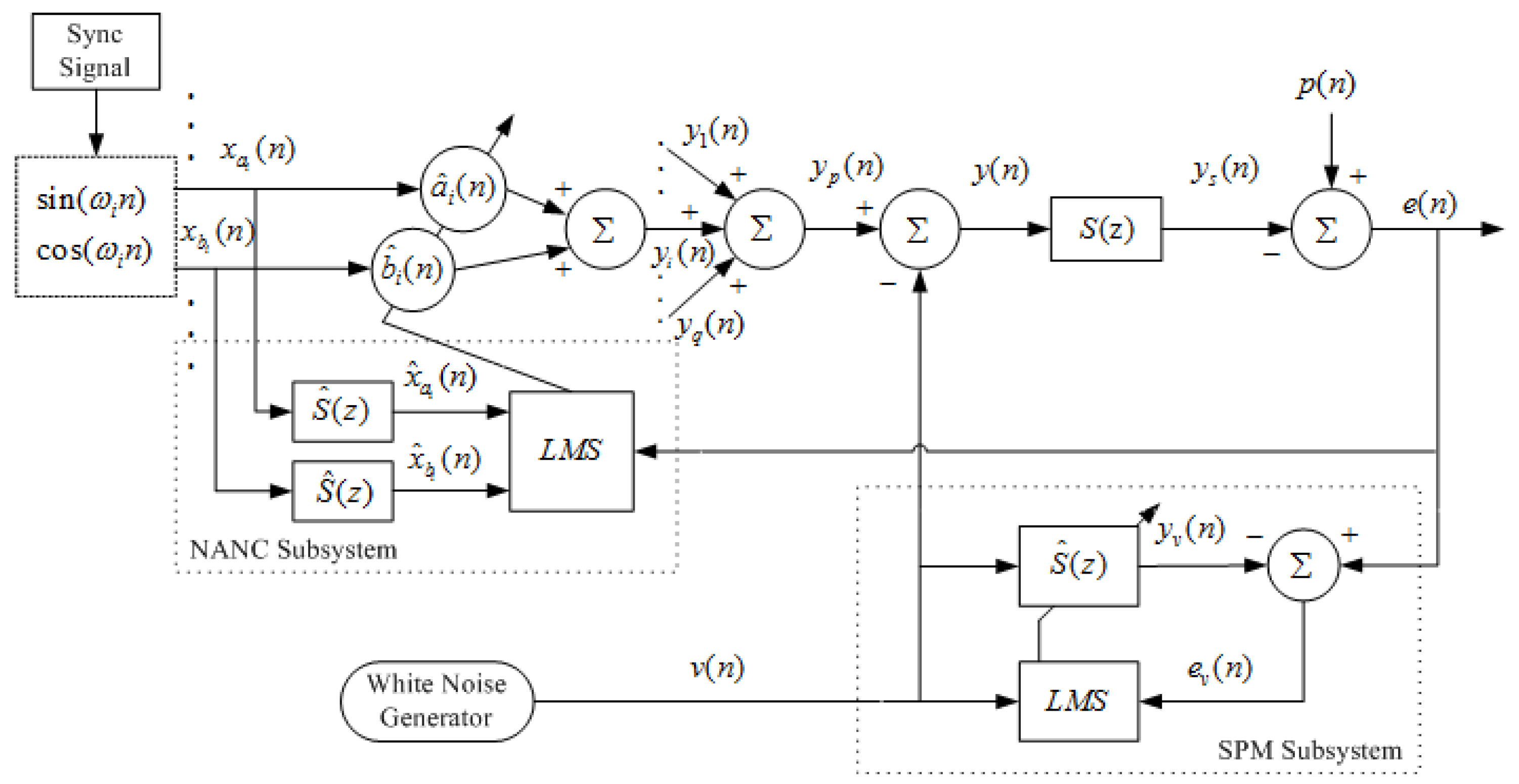
Figure 2.
NANC system with online SPM using scaled auxiliary noise injection (ith channel).

Figure 3.
NANC system with online SPM using new auxiliary noise power scheduling strategy (ith channel).
Figure 3.
NANC system with online SPM using new auxiliary noise power scheduling strategy (ith channel).
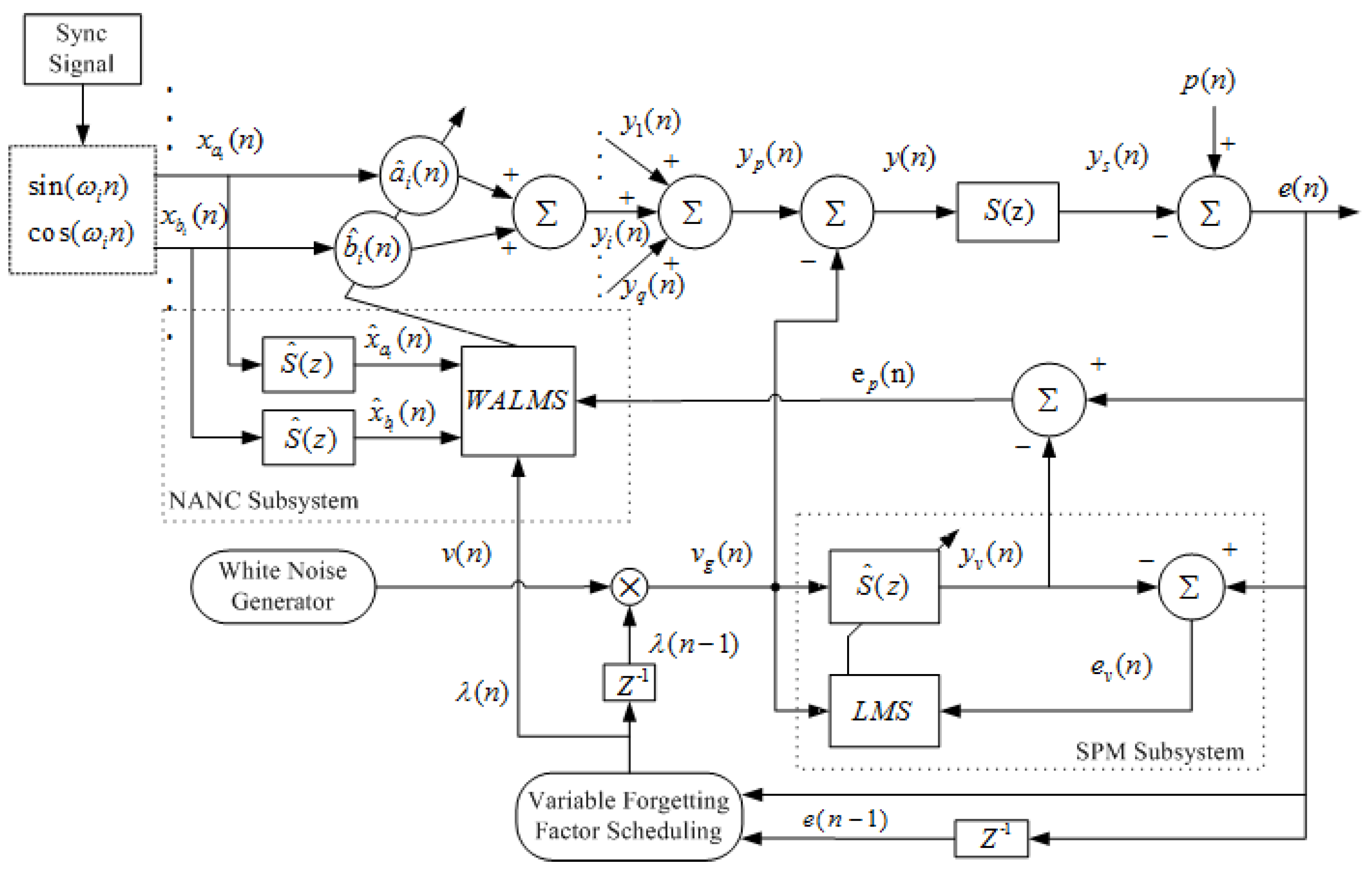
Figure 4.
Frequency response of the acoustic paths . (a) Original acoustic path; (b) Changed acoustic path at 50,000.
Figure 4.
Frequency response of the acoustic paths . (a) Original acoustic path; (b) Changed acoustic path at 50,000.

Figure 5.
Comparison between the discrete Fourier coefficient (DFC) estimation mean square errors (MSEs) of Method 1, Method 2, and the proposed method for the fixed acoustic path shown in Figure 4a. (a) ; (b) ; (c) ; (d) ; (e) ; (f) .
Figure 5.
Comparison between the discrete Fourier coefficient (DFC) estimation mean square errors (MSEs) of Method 1, Method 2, and the proposed method for the fixed acoustic path shown in Figure 4a. (a) ; (b) ; (c) ; (d) ; (e) ; (f) .
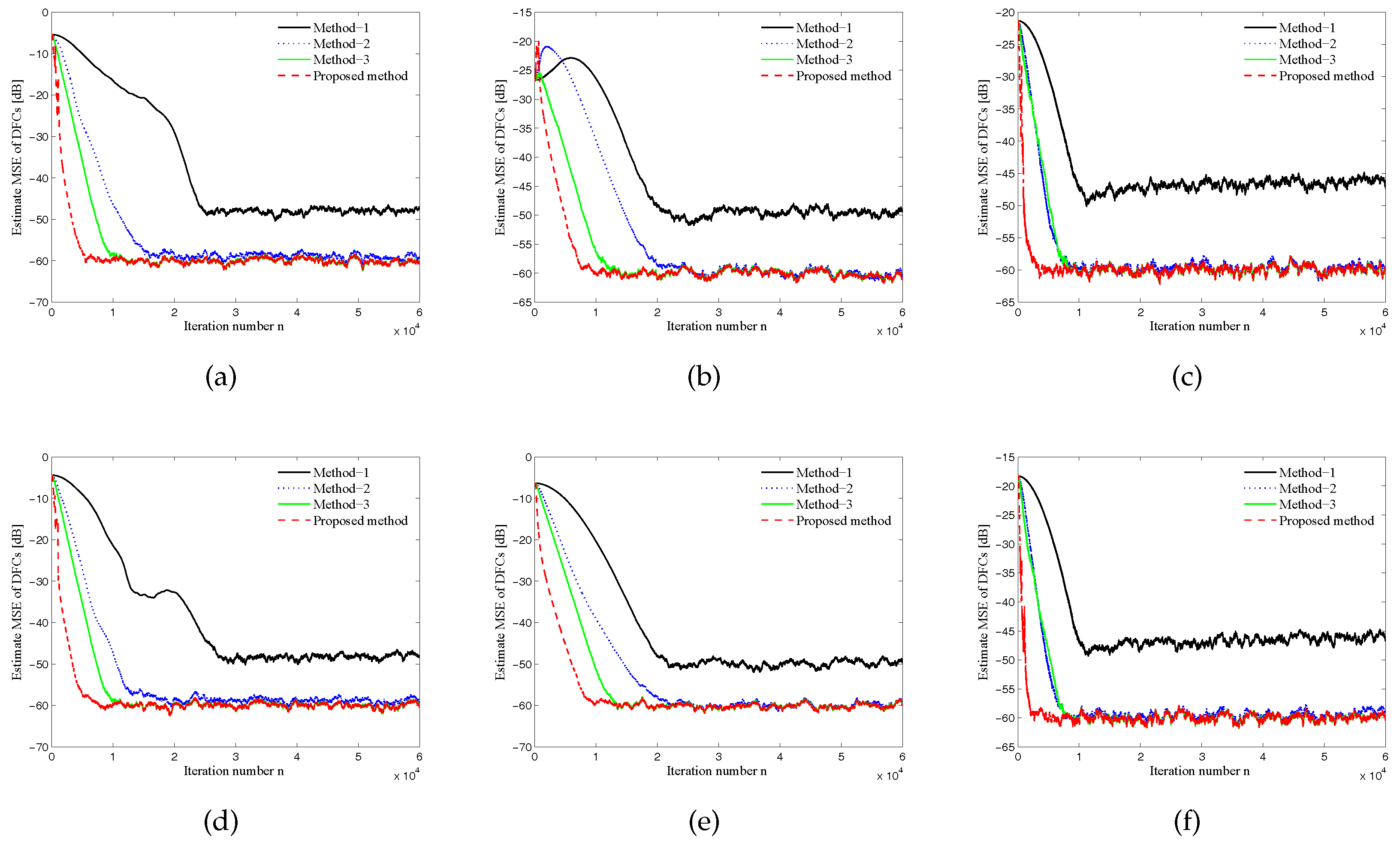
Figure 6.
Comparison between the residual errors of Method 1, Method 2, and the proposed method for the fixed acoustic path shown in Figure 4a. (a) Mean square error . (b) Mean square error obtained by averaging the square values of 50 past residue errors.
Figure 6.
Comparison between the residual errors of Method 1, Method 2, and the proposed method for the fixed acoustic path shown in Figure 4a. (a) Mean square error . (b) Mean square error obtained by averaging the square values of 50 past residue errors.
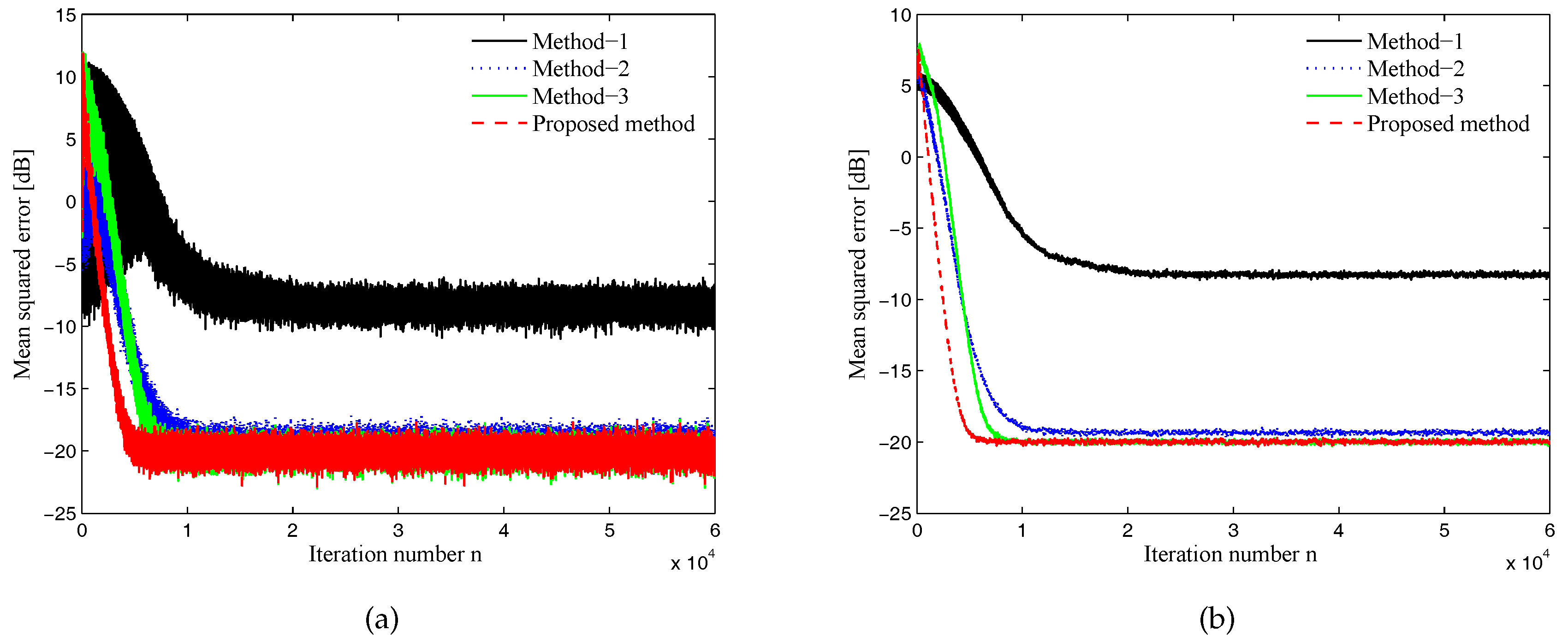
Figure 7.
Comparison between the modeling errors of Method 1, Method 2, and the proposed method for the fixed acoustic path shown in Figure 4a.
Figure 7.
Comparison between the modeling errors of Method 1, Method 2, and the proposed method for the fixed acoustic path shown in Figure 4a.

Figure 8.
Mean variable forgetting factor of the proposed method for the fixed acoustic path shown in Figure 4a.
Figure 8.
Mean variable forgetting factor of the proposed method for the fixed acoustic path shown in Figure 4a.

Figure 9.
Comparison between the DFC estimation MSEs of Method 1, Method 2, and the proposed method for the variable acoustic path shown in Figure 4. (a) ; (b) ; (c) ; (d) ; (e) ; (f) .
Figure 9.
Comparison between the DFC estimation MSEs of Method 1, Method 2, and the proposed method for the variable acoustic path shown in Figure 4. (a) ; (b) ; (c) ; (d) ; (e) ; (f) .

Figure 10.
Comparison between the residual errors of Method 1, Method 2, and the proposed method for the variable acoustic path shown in Figure 4. (a) Mean square error . (b) Mean square error obtained by averaging the square values of 50 past residue errors.
Figure 10.
Comparison between the residual errors of Method 1, Method 2, and the proposed method for the variable acoustic path shown in Figure 4. (a) Mean square error . (b) Mean square error obtained by averaging the square values of 50 past residue errors.
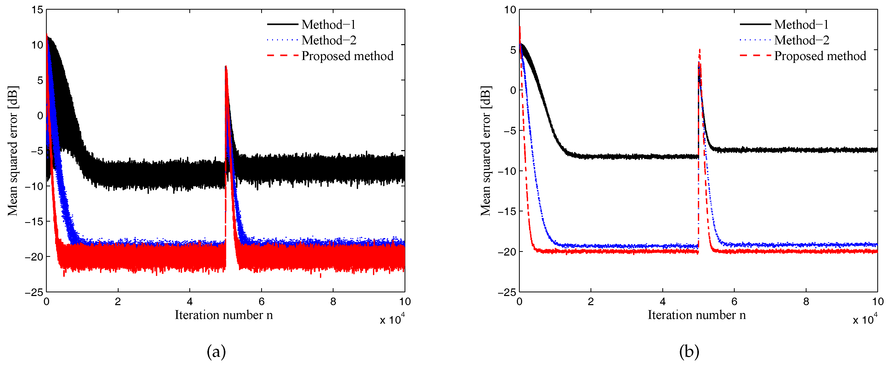
Figure 11.
Comparison between the modeling errors of Method 1, Method 2, and the proposed method for the variable acoustic path shown in Figure 4.
Figure 11.
Comparison between the modeling errors of Method 1, Method 2, and the proposed method for the variable acoustic path shown in Figure 4.

Figure 12.
Mean variable forgetting factor of the proposed method for the variable acoustic path shown in Figure 4.
Figure 12.
Mean variable forgetting factor of the proposed method for the variable acoustic path shown in Figure 4.

© 2017 by the authors. Licensee MDPI, Basel, Switzerland. This article is an open access article distributed under the terms and conditions of the Creative Commons Attribution (CC BY) license (http://creativecommons.org/licenses/by/4.0/).
Share and Cite
MDPI and ACS Style
Sun, C.; Liu, Y.; Bo, Z.; Jiang, S. A New Online Secondary Path Modeling Method with An Auxiliary Noise Power Scheduling Strategy for Narrowband Active Noise Control Systems. Appl. Sci. 2017, 7, 1236. https://doi.org/10.3390/app7121236
AMA Style
Sun C, Liu Y, Bo Z, Jiang S. A New Online Secondary Path Modeling Method with An Auxiliary Noise Power Scheduling Strategy for Narrowband Active Noise Control Systems. Applied Sciences. 2017; 7(12):1236. https://doi.org/10.3390/app7121236
Chicago/Turabian StyleSun, Chao, Yuqi Liu, Zhong Bo, and Shouda Jiang. 2017. "A New Online Secondary Path Modeling Method with An Auxiliary Noise Power Scheduling Strategy for Narrowband Active Noise Control Systems" Applied Sciences 7, no. 12: 1236. https://doi.org/10.3390/app7121236
Note that from the first issue of 2016, this journal uses article numbers instead of page numbers. See further details here.