Multi-Fidelity Multi-Objective Efficient Global Optimization Applied to Airfoil Design Problems

Abstract

In this study, efficient global optimization (EGO) with a multi-fidelity hybrid surrogate model for multi-objective optimization is proposed to solve multi-objective real-world design problems. In the proposed approach, a design exploration is carried out assisted by surrogate models, which are constructed by adding a local deviation estimated by the kriging method and a global model approximated by a radial basis function. An expected hypervolume improvement is then computed on the basis of the model uncertainty to determine additional samples that could improve the model accuracy. In the investigation, the proposed approach is applied to two-objective and three-objective optimization test functions. Then, it is applied to aerodynamic airfoil design optimization with two objective functions, namely minimization of aerodynamic drag and maximization of airfoil thickness at the trailing edge. Finally, the proposed method is applied to aerodynamic airfoil design optimization with three objective functions, namely minimization of aerodynamic drag at cruising speed, maximization of airfoil thickness at the trialing edge and maximization of lift at low speed assuming a landing attitude. XFOILis used to investigate the low-fidelity aerodynamic force, and a Reynolds-averaged Navier–Stokes simulation is applied for high-fidelity aerodynamics in conjunction with a high-cost approach. For comparison, multi-objective optimization is carried out using a kriging model only with a high-fidelity solver (single fidelity). The design results indicate that the non-dominated solutions of the proposed method achieve greater data diversity than the optimal solutions of the kriging method. Moreover, the proposed method gives a smaller error than the kriging method.

1. Introduction

A high-cost computation function is required to solve aerodynamic design problems. In addition, real-world design problems often involve several objective functions [1,2]. For example, in aircraft design, it is necessary for a designer to account for not only the performance at a specific cruise condition, but also the performances at all operating speeds, including those during take-off and landing. Owing to these problems, several researchers have explored methods to reduce the computational costs of design optimization algorithms for multi- or many-objective optimization problems.

In aerodynamic evaluation, it is possible to select various physical computation models to solve a design problem [3]. For example, forces around an airfoil can be evaluated by a potential equation as a low-level computation [4]. Moreover, the Navier–Stokes equation can be employed as a high-level computation [5]. Given the advantage of the above-mentioned approach, a multi-fidelity approach combines two-fidelity data for optimization in order to improve the efficiency of the optimization process. Thus, approaches that include a multi-fidelity surrogate model have been widely studied [6,7,8] in aerospace engineering. Multi-fidelity methods for single-objective optimization based on the error estimation of response surfaces have been successfully applied to design low-boom supersonic jets [6]. Because the response surfaces [9] use simple concepts to construct the function, the multi-fidelity function based on the response surface is easy to construct. However, such methods are often associated with low accuracy because the response surface model cannot be optimized in situations involving an extremely small number of data points. A co-kriging model [7,8] has been extensively applied to combine multi-fidelity functions. In addition, it has been employed to solve an optimal single-objective airfoil design problem [7]. This method is beneficial for predicting a complicated landscape function. However, it is less optimal in predicting a smooth landscape function. Rethore proposed a multi-fidelity single-objective optimization process for wind turbine design [10,11]. This optimization process begins with the location of an optimal point of a low-fidelity function by using a genetic algorithm (GA). Then, an optimization with a high-fidelity function is performed using a gradient-based method. The optimum point of the low-fidelity function is used as a starting point. This method is beneficial, as it uses a basic optimization tool to solve the multi-fidelity optimization problem. However, it could fail to find an optimum high-fidelity function if the error between the low-fidelity and high-fidelity functions is large. Because the gradient-based method required many evolution functions to solve multi-objective optimization problems, the multi-fidelity optimization based on evolutionary computation combined with the gradient method would not reduce the computation time of the high-fidelity function. Thus, multi-fidelity approaches are expected to improve the efficiency.

An approach to multi-fidelity/multi-objective optimization involves a model reduction technique [12,13]. This technique has been applied to helicopter rotor blade design and airfoil design [13,14]. The application of this technique reduces the design parameter space for defining the possible design ranges based on a low-fidelity function. A high-fidelity function is then used to find the optimum design in the primary defined design range. The high-fidelity function is sampled by selecting the preferred design points, where the blade shows improved performance with respect to the baseline design, in order to ensure good diversity of the sample data, in addition to the initial point that is generated with the primary defined design range. However, this approach has the potential to obtain an unexpected optimal solution outside the parameter space given that the design ranges of the low-fidelity function are not always appropriate for the high-fidelity function. Fusi [15] used GA to find the optimum solution of low-fidelity data and selected the interesting points of the optimum solution using the low-fidelity data to find the optimum point of high-fidelity data of a hovering rotor airfoil design.

Efficient global optimization (EGO) [16] is a widely-used method that consists of kriging-model-based explorations. EGO involves additional sampling-procedure-based expected improvements (EIs) for improving the model accuracy. The EIs are defined for single-objective optimization. The expected hypervolume improvement (EHVI) algorithm [17,18] has been proposed to improve the non-dominated front defining the expectations of hypervolume improvements (HVI); it considers the model uncertainty, as well as the EIs. However, existing studies have not investigated the applicability of EHVI to multi-fidelity techniques. In this article, a multi-objective optimization process involving multi-fidelity/multi-objective EGO is proposed and investigated through the solutions of test functions and airfoil design problems. With respect to airfoil design problems, a low-fidelity function is used to construct a global model that can provide the global landscape of the function. Further, a high-fidelity function is used to evaluate local deviations. The global model, constructed by a radial basis function (RBF) [19,20] based on a database, is evaluated using low-fidelity models. Local variances are predicted using a correlation term of the kriging method. The study involves airfoil design problems with two and three objectives. The results of the optimization are compared with those of an ordinary kriging-based EHVI involving a single-fidelity approach.

2. Surrogate Models for Design Optimization

2.1. Kriging Method

An ordinary kriging method [21] predicts the unknown function $\widehat{y}\left(\mathbf{x}\right)$ as:

$$\widehat{y}\left(\mathbf{x}\right)=\mu +\epsilon \left(\mathbf{x}\right),$$

(1)

where $\mu$ is global model and $\epsilon \left(\mathbf{x}\right)$ is a local deviation. The sample points $\mathbf{x}$ are interpolated with Gaussian random function. The correlation between $Z\left(x_i\right)$ and $Z\left(x_j\right)$ is related to the distance between the two corresponding point $x_i$ and $x_j$. A local deviation $\epsilon \left(\mathbf{x}\right)$ is expressed as:

$$d({\mathbf{x}}_i,{\mathbf{x}}_j)=\sum _{k=1}^n{\theta }^k{|x_i^k-x_j^k|}^2,$$

(2)

where ${\theta }^k(0\le {\theta }^k\le \infty )$ is the k-th element of the correlation vector parameter and n is the number of the sample points. The correlation between the points $x_i$ and $x_j$ is defined as:

$$Corr\left[Z\left(x_i\right),Z\left(x_j\right)\right]=\exp \left[-d(x_i,x_j)\right].$$

(3)

The kriging prediction can be expressed as:

$$\widehat{y}\left(\mathbf{x}\right)=\mu +{\mathbf{r}}^{\mathrm{T}}{\mathbf{R}}^{-1}(\mathbf{F}-\widehat{\mu }),$$

(4)

where $Z\left(x_i\right)$ represents a local deviation from the global model [22], $\mathbf{F}={\left[f\left(x_1\right),f\left(x_2\right),f\left(x_3\right),\dots ,f\left(x_n\right)\right]}^{\mathrm{T}}$ is the value of the evaluated function at $\mathbf{X}=\{x_1,x_2,x_3,\dots ,x_n\}$, $\mathbf{R}$ denotes the $n\times n$ matrix whose $(i,j)$ entry is $Corr\left[Z\left(x_i\right),Z\left(x_j\right)\right]$ and $\mathbf{r}$ is the vector i-th element:

$$r_i\left(\mathbf{x}\right)=Corr\left[Z\left(x\right),Z\left(x^i\right)\right].$$

(5)

$\mu$ is assumed to be constant in the original kriging model, and $\widehat{\mu }$ is given by:

$$\widehat{\mu }={[\mu ,\mu ,\mu ,\dots ,\mu ]}^{\mathrm{T}},$$

(6)

where $\mu$ is defined as:

$$\mu =\frac{{\mathbf{1}}^{\mathrm{T}}{\mathbf{R}}^{-1}\mathbf{F}}{{\mathbf{1}}^{\mathrm{T}}{\mathbf{R}}^{-1}\mathbf{1}}.$$

(7)

The unknown parameter, $\theta$, for the kriging model can be estimated via maximum likelihood estimation (MLE):

$$Ln(\mu ,{\sigma }^2,\theta )=-\frac{n}{2}ln\left({\sigma }^2\right)-\frac{1}{2}ln\left(\right|\mathbf{R}\left|\right).$$

(8)

MLE is an m-dimensional unconstrained nonlinear optimization problem. In this article, a GA [23] is used to solve this problem. For a given $\theta ,{\sigma }^2$ can be defined as:

$${\sigma }^2=\frac{{(\mathbf{F}-\widehat{\mu })}^{\mathrm{T}}{\mathbf{R}}^{-1}(\mathbf{F}-\widehat{\mu })}{n}.$$

(9)

The mean square error $s^2\left(\mathbf{x}\right)$ at a point $\mathbf{x}$ of this function can be calculated using the following equation:

$$s^2\left(\mathbf{x}\right)=\sigma \left[1-{\mathbf{r}}^{\mathrm{T}}{\mathbf{R}}^{-1}\mathbf{r}+\frac{1-{\mathbf{1}}^{\mathrm{T}}{\mathbf{R}}^{-1}\mathbf{F}}{{\mathbf{1}}^{\mathrm{T}}{\mathbf{R}}^{-1}\mathbf{1}}\right],$$

(10)

where $\mathbf{1}$ denotes an n-dimensional unit vector.

2.2. Hybrid Surrogate Model for Multi-Fidelity Approach

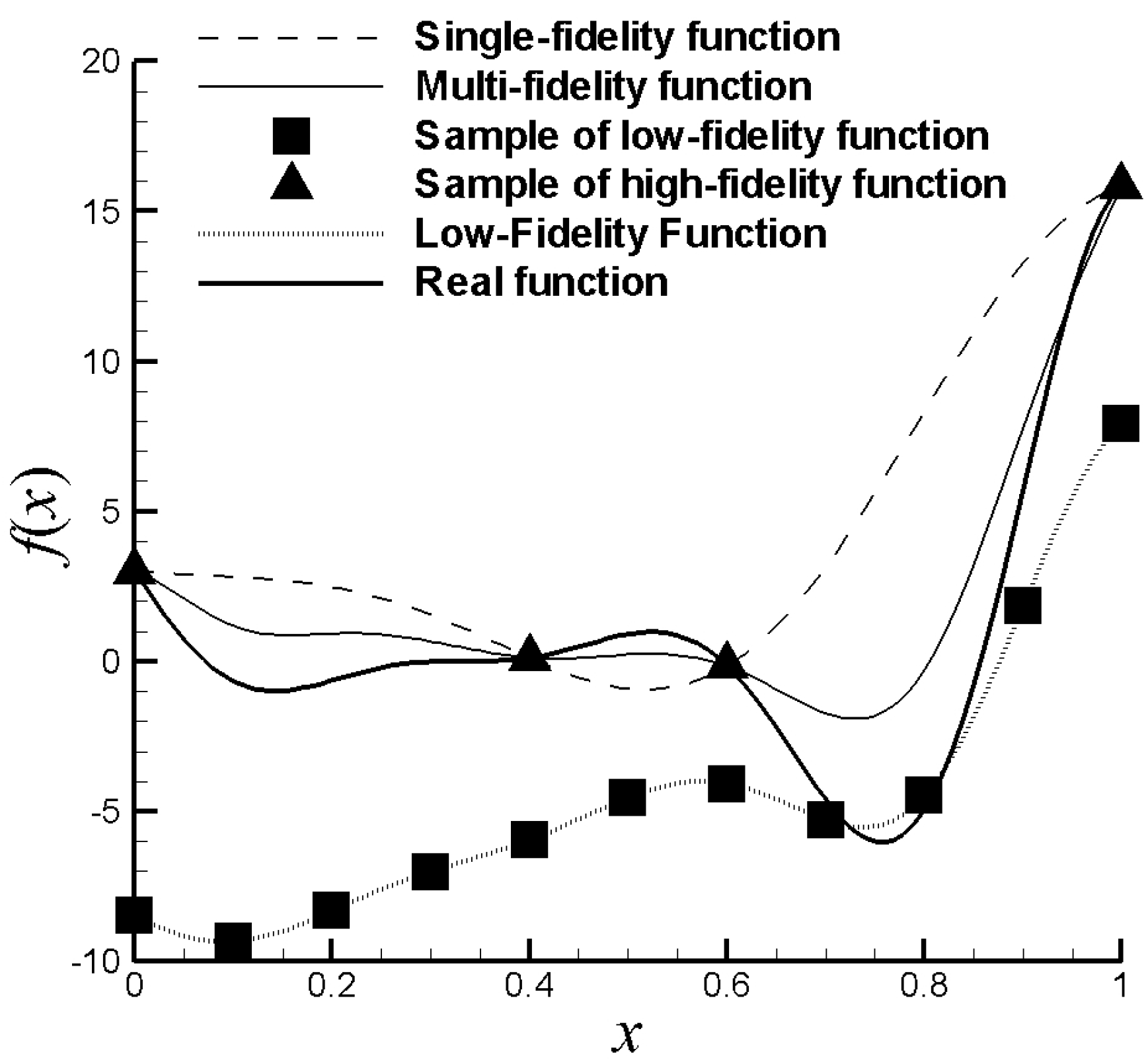
In this section, the hybrid surrogate model (Figure 1) is proposed for the multi-fidelity approach. The proposed approach constructed the local deviation estimated by the kriging method and the global model approximated by the RBF. It employs an RBF to represent the global model, $\mu +fr\left(\mathbf{x}\right)$, based on a dataset obtained from low-fidelity evaluation. The proposed approach combines the kriging method and the RBF by the following equation:

$$\widehat{y}\left(\mathbf{x}\right)=[\mu +fr\left(\mathbf{x}\right)]+{\mathbf{r}}^{\mathrm{T}}{\mathbf{R}}^{-1}({\mathbf{F}}_{\mathrm{h}}-\widehat{\mu }-\mathbf{FR}).$$

(11)

The local deviations ${\mathbf{r}}^{\mathrm{T}}{\mathbf{R}}^{-1}({\mathbf{F}}_{\mathrm{h}}-\widehat{\mu }-\mathbf{FR})$ are evaluated on the basis of a high-fidelity dataset using the kriging method, where ${\mathbf{F}}_{\mathrm{h}}={\left[f_{\mathrm{h}}\left(x_1\right),f_{\mathrm{h}}\left(x_2\right),f_{\mathrm{h}}\left(x_3\right),\dots ,f_{\mathrm{h}}\left(x_n\right)\right]}^{\mathrm{T}}$ is the value of the high-fidelity function at $\mathbf{x}=\{x_1,x_2,x_3,\dots ,x_n\}$; $\mathbf{FR}={\left[fr\left(x_1\right),fr\left(x_2\right),fr\left(x_3\right),\dots ,fr\left(x_n\right)\right]}^{\mathrm{T}}$, $fr\left(\mathbf{x}\right)$ the function predicted from the low-fidelity data that predicted by RBF, can be expressed by (12):

$$fr\left(\mathbf{x}\right)=a_0+a_1{f}_{\mathrm{l}}\left(\mathbf{x}\right),$$

(12)

where $f_{\mathrm{l}}\left(\mathbf{x}\right)$ is a function predicted by an RBF [19,20] using low-fidelity data and $a_0$ and $a_1$ are correlation terms between the low-fidelity data and the high-fidelity data. Further, ${\sigma }^2$ can be defined as:

$${\sigma }^2=\frac{{(\mathbf{F}-\widehat{\mu }-\mathbf{FR})}^{\mathrm{T}}{\mathbf{R}}^{-1}(\mathbf{F}-\widehat{\mu }-\mathbf{FR})}{n}.$$

(13)

The unknown parameters ($\theta ,a_0$ and $a_1$) for the hybrid surrogate multi-fidelity model can be estimated by MLE, as expressed by (8).

The RBF is used to approximate the global model of the hybrid surrogate-model. An RBF is used to predict the low-fidelity function ($f_{\mathrm{l}}\left(\mathbf{x}\right)$) by:

$$f_{\mathrm{l}}\left(\mathbf{x}\right)=\sum _{m=1}^n{w}_m\mathsf{\Phi }(\mathbf{x}-{\mathbf{x}}_m)$$

(14)

where $\mathsf{\Phi }\left(\mathbf{x}\right)$ is an RBF, ${\mathbf{x}}_m$ is a sample point and $w_m(m=1,2,3,\dots ,n)$ is a weighting function. A multi-quadratic function is applied as an RBF in this study. The weighting function $\mathbf{w}={[w_1,w_2,w_3,\dots ,w_n]}^{\mathrm{T}}$ is determined from the interpolation conditions:

$$A\mathbf{w}=\mathbf{F}$$

(15)

where $A=\left(\begin{array}{cccc}{a}_{1,1}& a_{1,2}& \cdots & a_{1,j}\\ a_{2,1}& a_{2,2}& \cdots & a_{2,j}\\ ⋮& ⋮& \ddots & ⋮\\ a_{i,1}& a_{i,2}& \cdots & a_{i,j}\end{array}\right)$, $a_{i,j}=\mathsf{\Phi }({\mathbf{x}}_i-{\mathbf{x}}_j),i=1,2,3,\dots ,n,j=1,2,3,\dots ,n$

Here, $\mathbf{F}={\left[f\left(x_1\right),f\left(x_2\right),f\left(x_3\right),\dots ,f\left(x_n\right)\right]}^{\mathrm{T}}$ is the value of the low-fidelity function at $\mathbf{X}=\{x_1,x_2,x_3,\dots ,x_n\}$.

3. Efficient Global Optimization for the Multi-Objective Problem

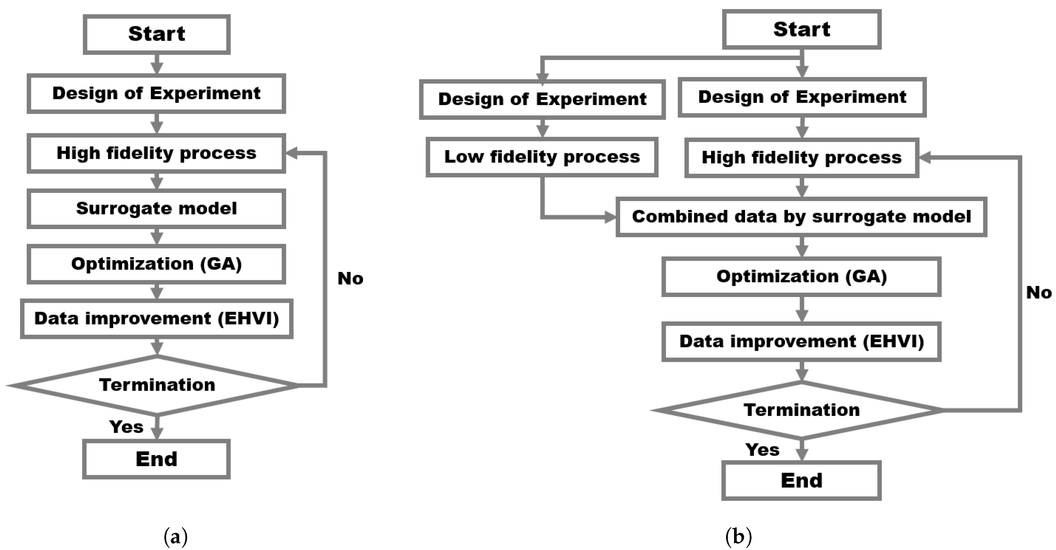
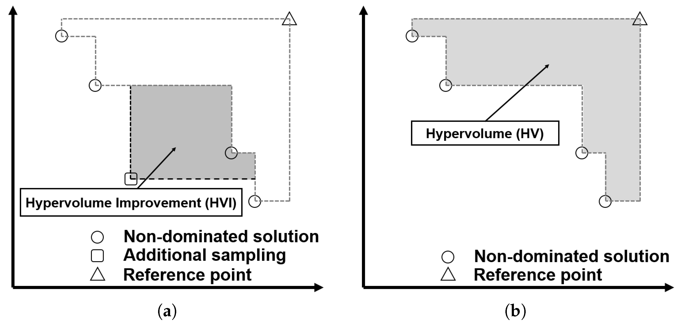
The procedure of EGO with the ordinary kriging model is illustrated in Figure 2a. The EGO process starts with the generated initial samples. In this study, the Latin hypercube sampling (LHS) is employed. Sample data are evaluated, and the model is predicted using the kriging method. An arbitrary optimization method can be used to find an additional point by maximizing an EHVI [17,18]. The EHVI is the function of the hypervolume improvement (HVI) combined with the uncertainty of the additional point. HVI is calculated from the hypervolume improvement of the additional sampling and the non-dominated solution shown in Figure 3a.

The EHVI at a point can be expressed as:

$$\begin{array}{c}EHVI[f_1\left(\mathbf{x}\right),f_2\left(\mathbf{x}\right),\dots ,f_M\left(\mathbf{x}\right)]=\hfill \\ {\int }_{-\infty }^{f_{ref1}}{\int }_{-\infty }^{f_{ref2}}\dots {\int }_{-\infty }^{f_{refM}}HVI[f_1\left(\mathbf{x}\right),f_2\left(\mathbf{x}\right),\dots ,f_M\left(\mathbf{x}\right)]\times {\varphi }_1\left(F_1\right){\varphi }_2\left(F_2\right)\dots {\varphi }_M\left(F_M\right)d{F}_{1}d{F}_2\dots d{F}_M,\hfill \end{array}$$

(16)

where $F_i$ denotes the Gaussian random variable $N[{\widehat{f}}_i\left(\mathbf{x}\right),{\widehat{s}}_i^2\left(\mathbf{x}\right)]$. ${\varphi }_i\left(F_i\right)$ is the probability density function and $f_{refi}$ is the reference value used for calculating the hypervolume. The maximization of EHVI is considered as the updating criterion to determine the location of an additional sample point. In this study, the hypervolume is calculated based on the HypEalgorithm [24], which is an algorithm that uses the Monte Carlo simulation [25] to approximate the hypervolume for multi/many-objective optimization problems. The Monte Carlo simulation is one of the simplest ways to calculate the hypervolume (HV) for many dimensions, which is often difficult to calculate. Thus, the HypE algorithm uses the benefit of the Monte Carlo simulation to calculate the hypervolume. The hypervolume is the volume of the non-dominated solutions measured from the reference point. The schematic illustration of the hypervolume is shown in Figure 3b.

The basic idea of the original EGO, namely EHVI-based explanation, can also be applied to the hybrid surrogate model expressed in (10), because local deviations are estimated using the kriging method. The procedure of EGO with the hybrid surrogate model proposed in this study is shown in Figure 2b. The proposed hybrid surrogate-model-based EGO starts by acquiring initial samples for a low-fidelity/low-cost function. The low-fidelity sample data are used to predict the global model; then, a set of samples for a high-fidelity function is obtained. This result is used to estimate the local deviations using the kriging method. Then, the multi-fidelity surrogate model, which can predict the unknown point value (an approximation of the high-fidelity function), is generated. A GA [23] is used to find the maximum EHVI point, x. In this study, the roulette wheel method was used in the selection process. Blend crossover (BLX)-0.5 [26] was used in the crossover process, and uniform mutation [27] with a mutation rate of 0.1 was used in the mutation process.

4. Investigation of Proposed Method by Solving Test Functions

4.1. Formulation

The proposed multi-objective multi-fidelity EGO is investigated by solving two test functions; one has two objective functions, and the other has three objective functions. The results are compared with those of a kriging-based multi-objective EGO. The high-fidelity function is denoted by f, and the low-fidelity function is denoted by $f_{\mathrm{l}}$.

The definition of two-objective optimization problem from Van Valedhuizen’s test suite [28] is:

$$\begin{array}{c}\mathrm{Minimize}:f_1(x_1,x_2,\dots ,x_5)=1-\exp \left(-\sum _{i=1}^5{(x_i-1/\sqrt{5})}^2\right)\hfill \\ \mathrm{Minimize}:f_2(x_1,x_2,\dots ,x_5)=1-\exp \left(-\sum _{i=1}^5{(x_i+1/\sqrt{5})}^2\right)\hfill \\ f_{\mathrm{l}1}(x_1,x_2,\dots ,x_5)=1-\exp \left(-\sum _{i=1}^5{(0.5x_i-0.05-1/\sqrt{5})}^2\right)\hfill \\ f_{\mathrm{l}2}(x_1,x_2,\dots ,x_5)=1-\exp \left(-\sum _{i=1}^5{(0.75x_i+0.2+1/\sqrt{5})}^2\right).\hfill \end{array}$$

(17)

The design space of this problem is $x_1,x_2,\dots ,x_5\in [-2.5,2.5]$.

The definition of the DTLZ2 three-objective optimization problem [28] is:

$$\begin{array}{c}\mathrm{Minimize}:f_1(x_1,x_2,\dots ,x_5)=(1+g)\cos \left(0.5x_i\pi \right)\cos \left(0.5x_2\pi \right)\hfill \\ \mathrm{Minimize}:f_2(x_1,x_2,\dots ,x_5)=(1+g)\cos \left(0.5x_1\pi \right)\sin \left(0.5x_2\pi \right)\hfill \\ \mathrm{Minimize}:f_3(x_1,x_2,\dots ,x_5)=(1+g)\sin \left(0.5x_1\pi \right)\hfill \\ g=\sum _{i=3}^5{(x_i-0.5)}^2\hfill \\ f_{\mathrm{l}1}(x_1,x_2,\dots ,x_5)=(0.5+1.5g_c)\cos \left(0.6x_i\pi \right)\cos \left(0.4x_2\pi \right)\hfill \\ f_{\mathrm{l}2}(x_1,x_2,\dots ,x_5)=(0.3+1.2g_c)\cos \left(0.4x_1\pi \right)\sin \left(0.6x_2\pi \right)\hfill \\ f_{\mathrm{l}3}(x_1,x_2,\dots ,x_5)=(0.4+1.3g_c)\sin \left(0.5x_1\pi \right)\hfill \\ g_c=\sum _{i=3}^5{(0.8x_i-0.3)}^2.\hfill \end{array}$$

(18)

The design space of this problem is $x_1,x_2,\dots ,x_5\in [0,1]$.

In each investigation, 10 initial high-fidelity points, f, and 150 low-fidelity points, $f_{\mathrm{l}}$, were acquired by LHS. The number of iterations was set to 30 for each test function.

4.2. Two-Objective Test Function Results

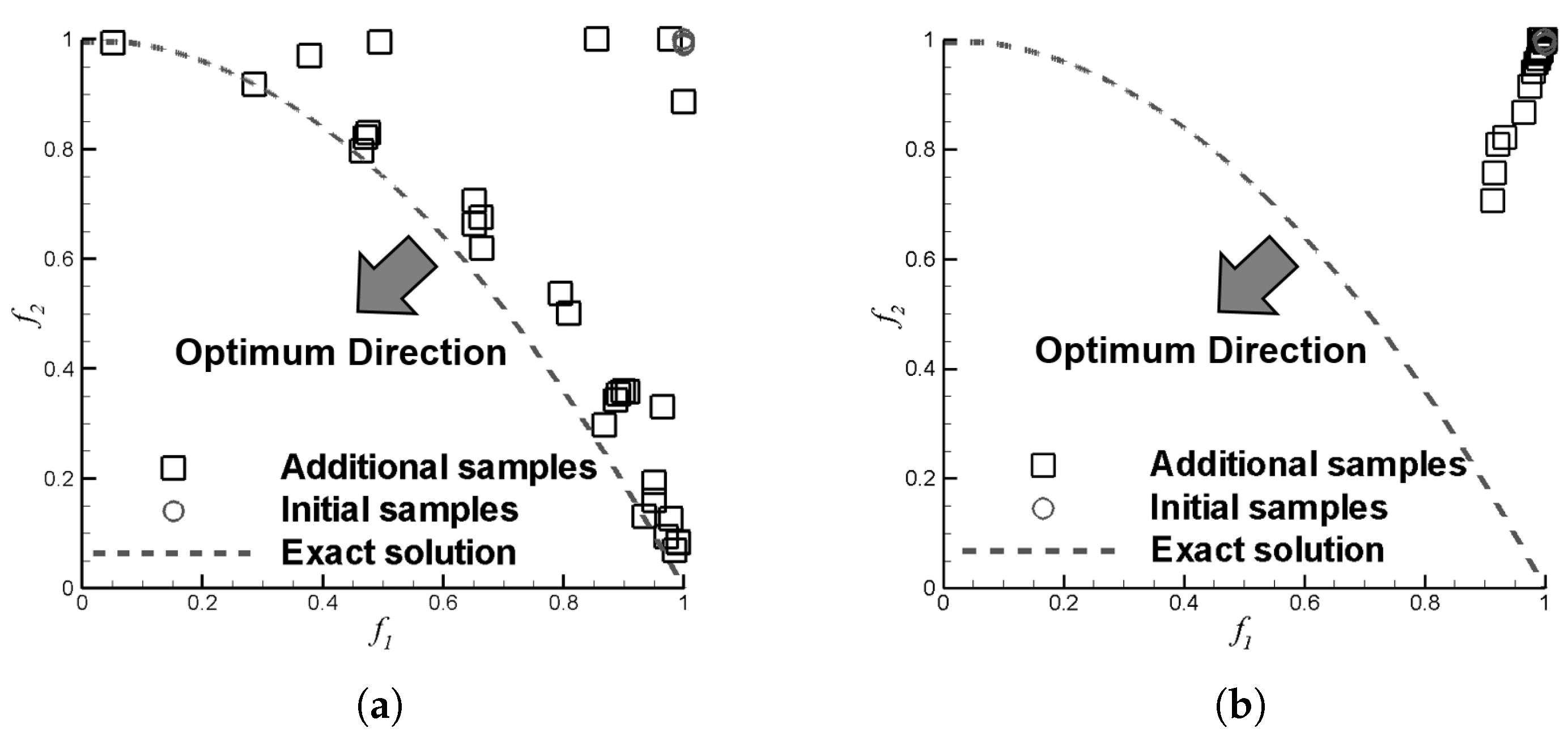
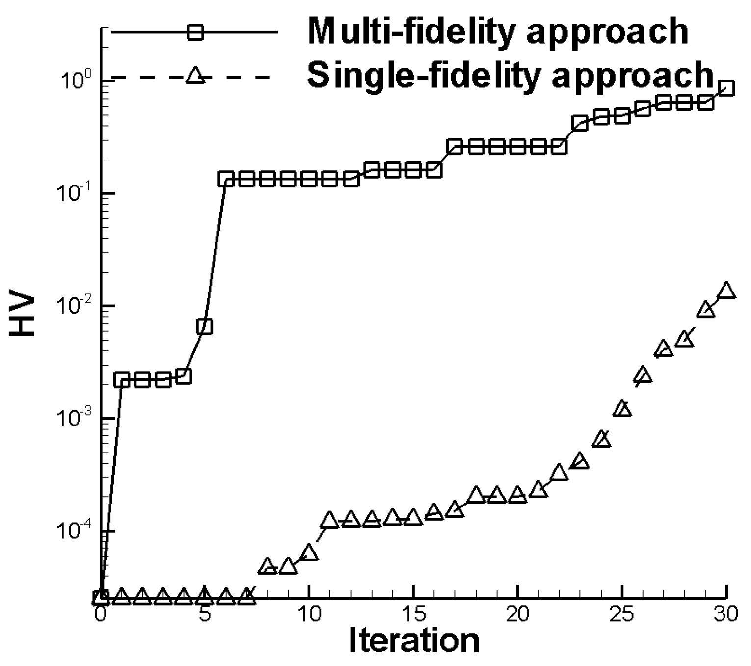
The solution space acquired by the proposed multi-fidelity/multi-objective EGO is compared with that acquired by the single-fidelity/multi-objective EGO as shown in Figure 4. Because the single-fidelity/multi-objective EGO finds local optimum points at the beginning of the optimization process, the solution for additional samples stalls earlier. On the other hand, the developed multi-fidelity/multi-objective EGO can find a solution close to the global optimum solution of this multi-objective optimization problem. The histories of the hypervolumes of the two methods are compared in Figure 5. These results also indicate that the proposed multi-fidelity/multi-objective EGO provides better solutions, which shows higher diversity because its hypervolume is larger than that of the single-fidelity/multi-objective EGO. These results also suggest that the proposed multi-fidelity/multi-objective EGO obtains better solutions than the single-fidelity/multi-objective EGO, because the non-dominated solutions of the former can dominate all the non-dominated solutions of the latter. In addition, comparisons of the hypervolumes show that the solution of additional samples by the single-fidelity/multi-objective EGO continues to stall earlier.

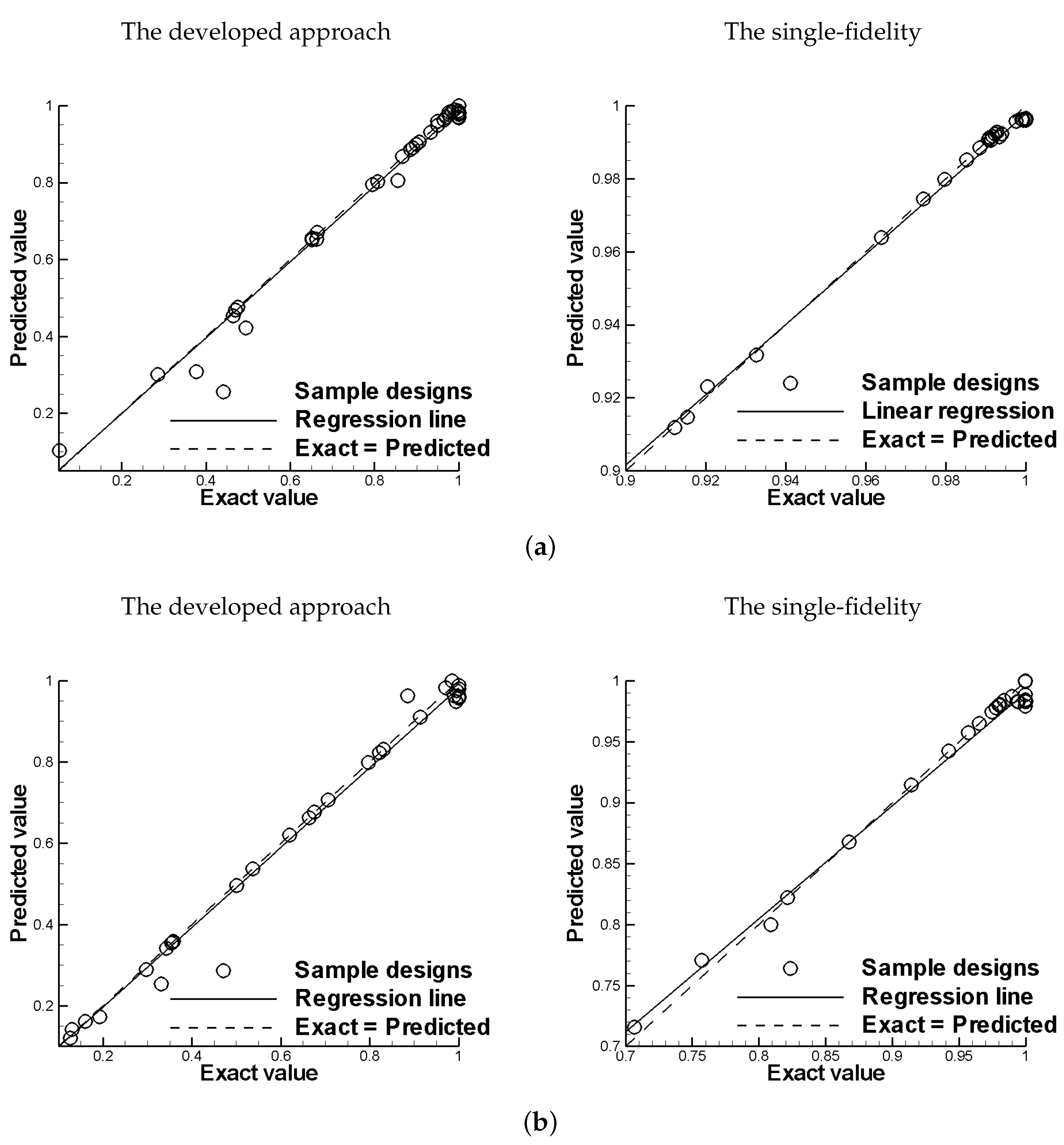
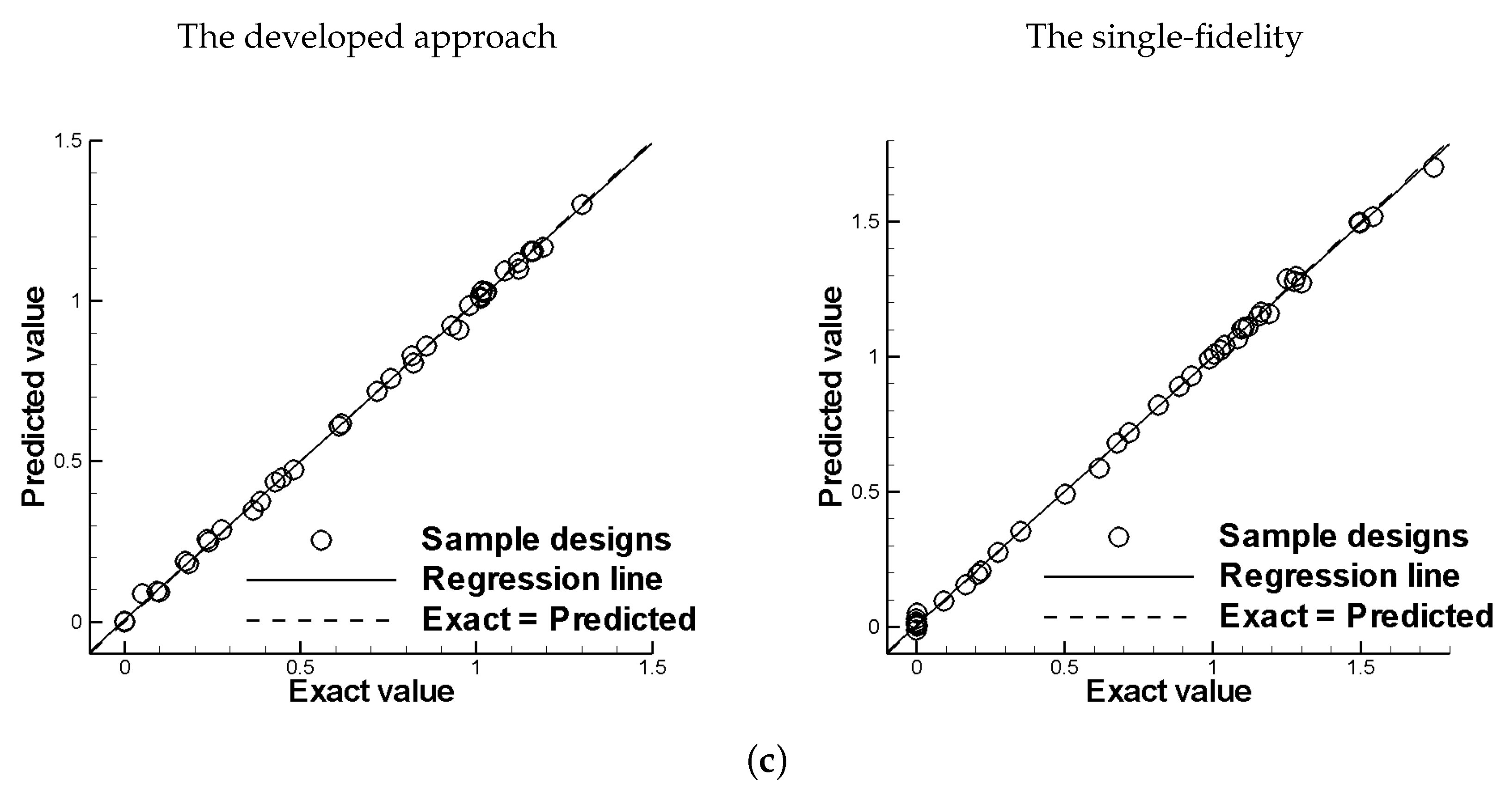
To investigate the reason for the superiority of the proposed multi-fidelity/multi-objective EGO, the cross-validation [29,30] of $f_1$ and $f_2$ was compared, as shown in Figure 6. It can be seen that the linear regression line nearly coincides with the predicted line in the case of the proposed multi-fidelity/multi-objective EGO. Thus, the multi-fidelity surrogate model achieves higher accuracy than the single-fidelity surrogate model. More specifically, the proposed multi-fidelity/multi-objective EGO achieves higher accuracy because the dataset obtained by low-fidelity evaluation enables the surrogate model to predict the solution in the uncertainty region.

4.3. Three-Objective Test Function Results

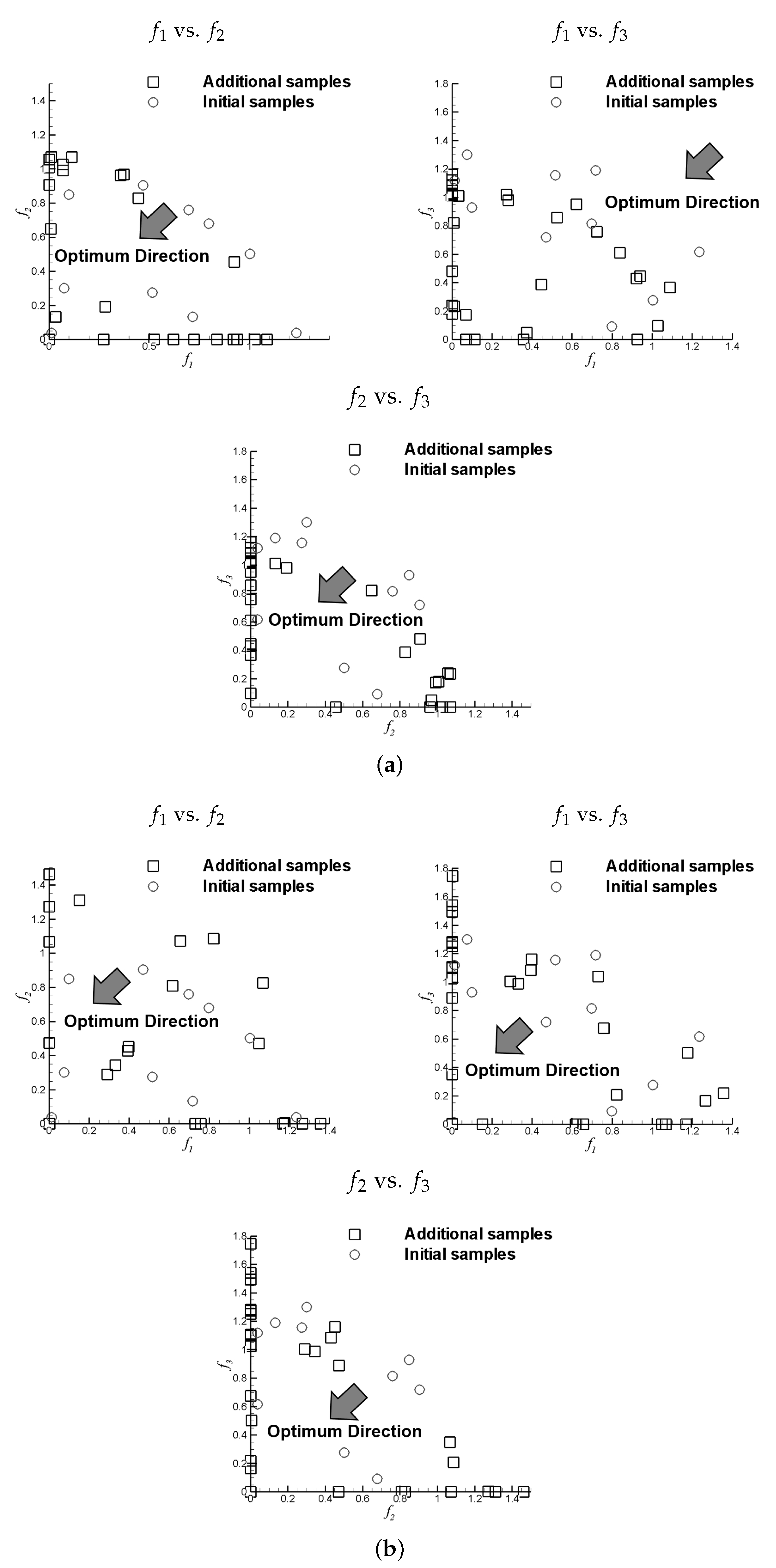
Further, all the samples acquired by the two methods (the proposed multi-fidelity/multi-objective EGO and the single-fidelity/multi-objective EGO) are compared as shown in Figure 7. According to these results, the proposed multi-fidelity/multi-objective EGO and the single-fidelity/multi-objective EGO have similar non-dominated solutions. However, the results of the multi-fidelity/multi-objective EGO are better than those of the single-fidelity/multi-objective EGO because some of the results of additional sampling by the single-fidelity/multi-objective EGO stall at local optimum points. The hypervolumes of the two methods are compared in Figure 8. The hypervolume comparison of the proposed multi-fidelity/multi-objective EGO and single-fidelity/multi-objective EGO is shown in Figure 9. It suggests that the proposed multi-fidelity/multi-objective EGO gives better solutions than that of the single-fidelity/multi-objective EGO. These results indicate that the proposed multi-fidelity/multi-objective EGO has a higher convergence rate than the single-fidelity/multi-objective EGO. The solution of the proposed multi-fidelity/multi-objective EGO converges after 18 iterations with a larger hypervolume, whereas the solution of the single-fidelity/multi-objective EGO converges after 23 iterations.

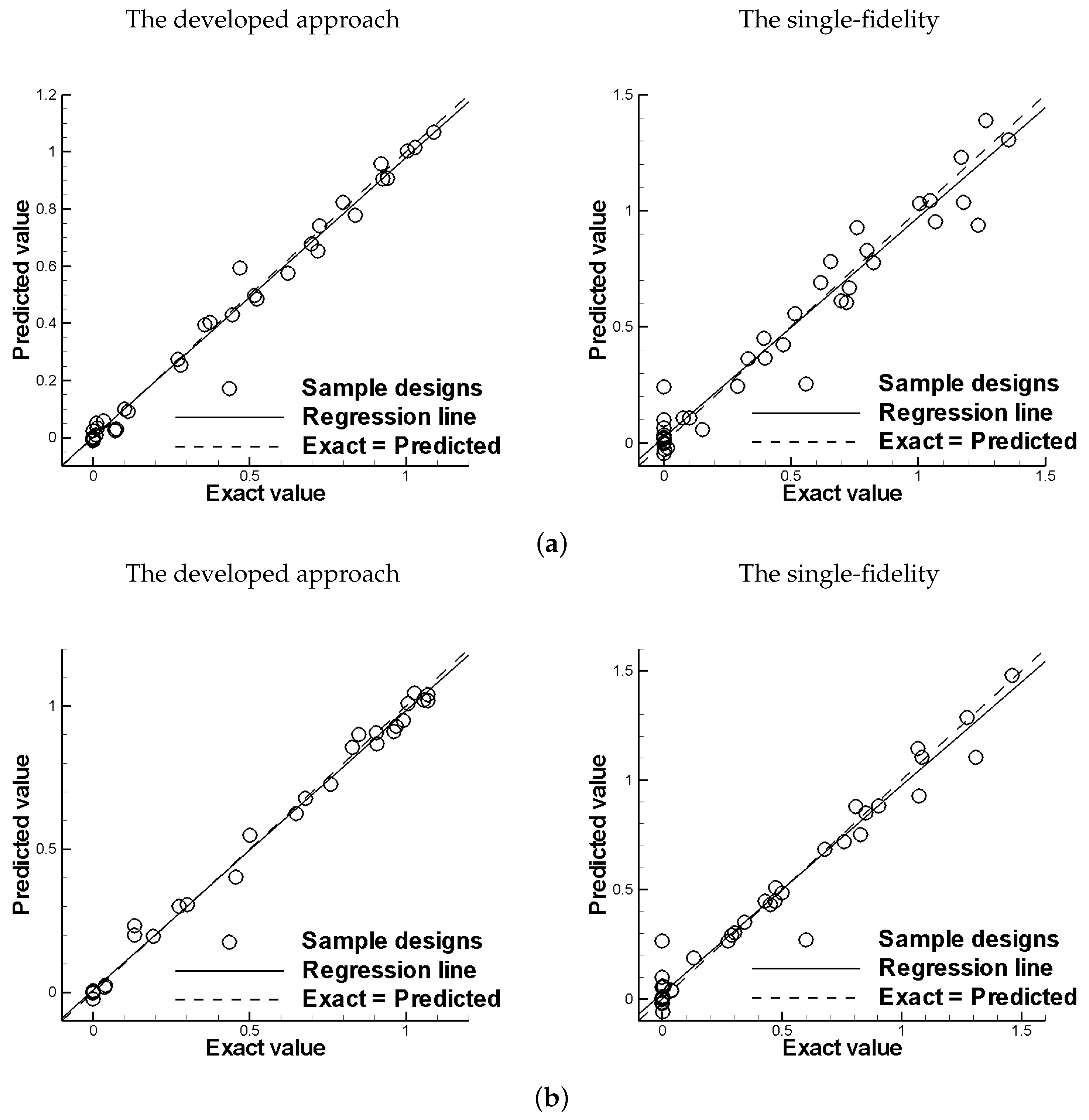
The cross-validation results for $f_1$, $f_2$ and $f_3$ are shown in Figure 9. The results indicate that the multi-fidelity surrogate model can achieve higher accuracy than the single-fidelity surrogate model for $f_1$ and $f_2$. Moreover, the results show that the non-dominated solution of the multi-fidelity/multi-objective EGO has a higher convergence rate because of the higher accuracy of the multi-fidelity surrogate model. With regard to $f_3$, a comparison between the multi-fidelity and single-fidelity surrogate models shows that the two methods have similar accuracy because $f_3$ has a simpler shape than $f_1$ and $f_2$.

5. Airfoil Design Problem

The proposed multi-fidelity/multi-objective design method discussed in Section 3 was also investigated by solving two airfoil design problems as real-world design problems.

5.1. Formulations

5.1.1. Two-Objective Case

The first problem has two objectives: minimize the aerodynamic drag ($C_{\mathrm{d}}$) at Mach 0.3, which requires a target lift of 0.5, and maximize the airfoil thickness at 75.0% of the chord length ($t_{75}$), which can be obtained directly by the real function because it can be calculated rapidly. Thus, two surrogate models are constructed. The optimization problem can be expressed as:

$$\begin{array}{c}\mathrm{Minimize}:C_{\mathrm{d}}\mathrm{at}Re=4\times {10}^6,Ma=0.3,C_{\mathrm{l}}=0.5\hfill \\ \mathrm{Maximize}:t_{75}\hfill \end{array}$$

(19)

The number of initial samples for the high-fidelity/high-cost function is set to 10, and the number of low-fidelity/low-cost functions for the multi-fidelity surrogate model is 150. Further, the number of additional samples for this problem is set to 30. $t_{75}$ can be immediately calculated after the set of design parameters is decided upon. Thus, we used the exact value for $t_{75}$ in the following equation based on Equation (16).

$$EHVI={\int }_{-\infty }^{C_{\mathrm{d},\max }}HVI[C_{\mathrm{d}},t_{75}]\times {\varphi }_1\left(C_{\mathrm{d}}\right)d{C}_{\mathrm{d}}.$$

(20)

5.1.2. Three-Objective Case

The second problem has three objectives: minimize $C_{\mathrm{d}}$ at cruising speed, maximize $t_{75}$ and maximize the lift coefficient ($C_{\mathrm{l}}$) in the landing condition at an angle of attack of 5.0${}^{\circ }$. The optimization problem is expressed as:

$$\begin{array}{c}\mathrm{Minimize}:C_{\mathrm{d}}\mathrm{at}Re=4\times {10}^6,Ma=0.3,C_{\mathrm{l}}=0.5\hfill \\ \mathrm{Maximize}:C_{\mathrm{l}}\mathrm{at}Re=2\times {10}^6,Ma=0.15,\alpha =5.0^{\mathrm{o}}\hfill \\ \mathrm{Maximize}:t_{75}\hfill \end{array}$$

(21)

In this problem, the hybrid surrogate model is used to predict $C_{\mathrm{d}}$ and $C_{\mathrm{l}}$. Further, $t_{75}$ can be directly obtained by the real function. The number of initial samples for the high-fidelity/high-cost function is set to 10, and the number of low-fidelity/low-cost functions for the multi-fidelity surrogate model is 150. Further, the number of additional samples for this problem is set to 30. $t_{75}$ can be immediately calculated after the set of design parameters is decided upon. Thus, we used the exact value for $t_{75}$ in the following equation based on Equation (16).

$$EHVI={\int }_{-\infty }^{C_{\mathrm{d},\max }}{\int }_{C_{\mathrm{l},\min }}^{\infty }HVI[C_{\mathrm{d}},t_{75},C_{\mathrm{l}}]\times {\varphi }_1\left(C_{\mathrm{d}}\right){\varphi }_2\left(C_{\mathrm{l}}\right)d{C}_{\mathrm{d}}d{C}_{\mathrm{l}}.$$

(22)

5.2. Evaluation Methods

5.2.1. High-Fidelity Evaluation Using CFD as the High-Cost Function

The aerodynamic evaluation as a high-fidelity function was carried out using a Reynolds-averaged Navier–Stokes (RANS) solver [31]. The governing equation is expressed as:

$$\frac{\partial }{\partial T}{\int }_{\mathsf{\Omega }}\mathsf{\Psi }dV+{\oint }_{\partial \mathsf{\Omega }}Q·nds=0,$$

(23)

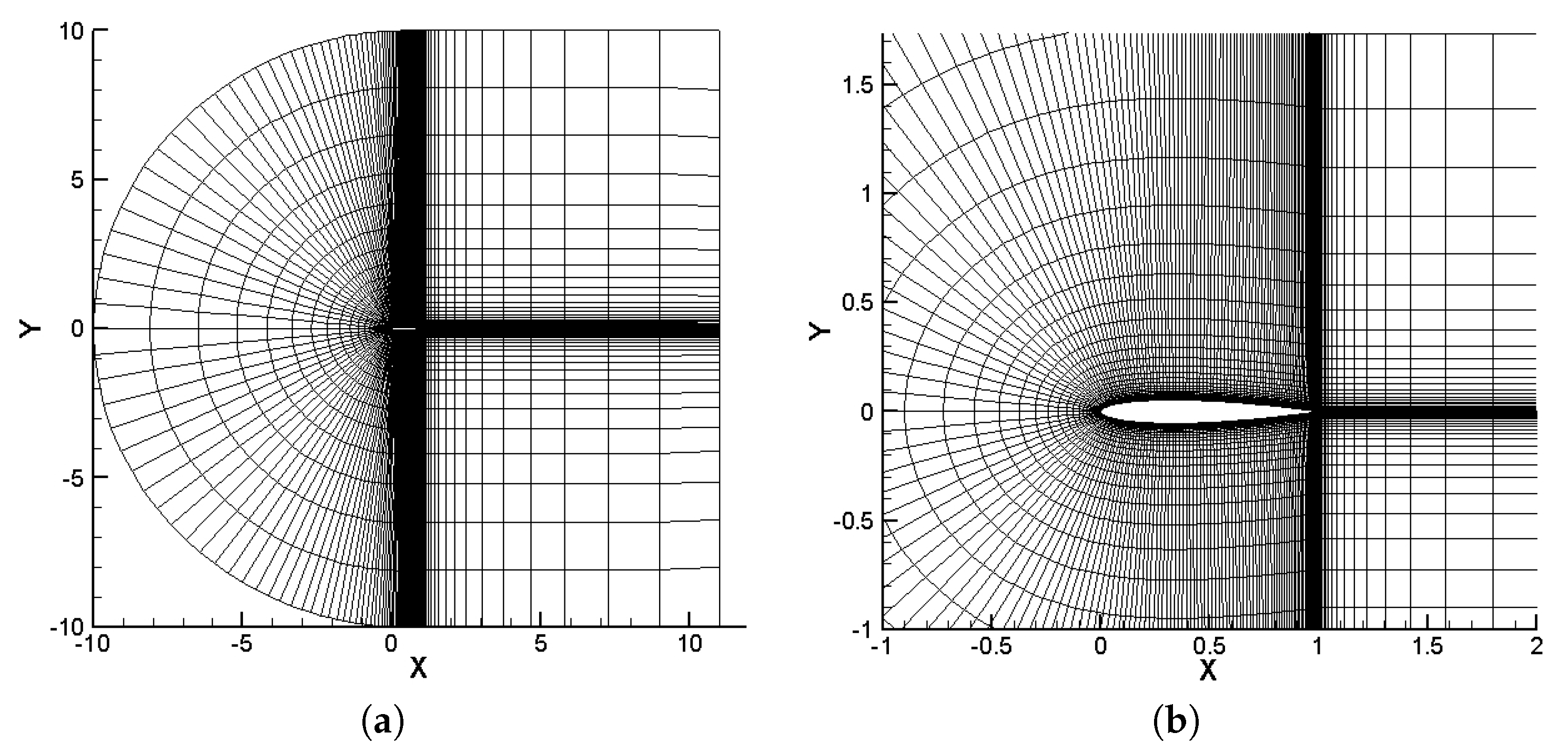
$\mathsf{\Psi }$ is a vector that consists of conservative quantities, and Q is the summation of conservative quantities entering and leaving the area. A lower-upper symmetric Gauss–Seidel (LU-SGS) implicit method [32] was employed for time integration, and a third-order-accurate upwind difference scheme with a monotone upstream-centered scheme for conservation laws (MUSCL) method [33] was employed for the flux evaluation. Further, the Baldwin–Lomax model [34] was used as a turbulent model. In addition, a structured grid was automatically created by an algebraic method for each design ($200\times 61$ structured grid for the RANS solver, as shown in Figure 10). The computation time of CFD in this work is approximately 180 to 300 s.

5.2.2. Low-Fidelity Solver as the Low-Cost Function

XFOIL [35] was employed as the low-fidelity evaluation. In XFOIL, the inviscid pressure distribution is modeled using a linear vortex strength distribution, while the viscous effects and the development of the laminar-turbulent boundary layer are modeled using integral boundary layer theory. The computation time of XFOIL is approximately 1 to 2 s.

5.2.3. Airfoil Representation

In this study, the class-shape function transformation (CST) parameterization method [36] was used for airfoil shape parameterization. The benefits of CST are that it could can generate several kinds of aerodynamic shapes and that it has a high degree of freedom due to the changeable number of numbers of the controlled parameter to generate the airfoil shape; whereas the other type of airfoil representation, such as NACA’s airfoil representation, parametric section (PARSEC) and non-uniform rational B-spline (NURBS), have the fixed controlled parameters. The product of a class function, $C(x/c)$, and a shape function, $S(x/c)$, can be represented geometrically by adding a term that characterizes the trailing edge thickness:

$$\frac{y}{c}=C\left(\frac{x}{c}\right)S\left(\frac{x}{c}\right)+\frac{x}{c}\frac{\Delta z_{te}}{c},$$

(24)

where $\Delta z_{te}$ is the trailing edge thickness, and $C(x/c)$ is given in generic form by:

$$C\left(\frac{x}{c}\right)\equiv {\left(\frac{x}{c}\right)}^{N_1}{\left[1-\frac{x}{c}\right]}^{N_2}\mathrm{for}0\le \frac{x}{c}\le 1.$$

(25)

The shape function, $S(x/c)$, is defined on the basis of the Bernstein binomials [37], by the introduction of weight factor $b_i$ as follows:

$$S\left(\frac{x}{c}\right)=\sum _{i=0}^n\left[b_i·K_{i,p}·{\left(\frac{x}{c}\right)}^i·{\left(1-\frac{x}{c}\right)}^{p-i}\right],$$

(26)

where p is the degree of the Bernstein binomials. In this study, $N_1$ was set to 0.5 and $N_2$ was set to 1.0. Further, third-degree Bernstein polynomials were used to generate the airfoil shape for the lower side $b_1-b_3$ and the upper side $b_4-b_6$. The ranges of the design parameters are defined in

Table 1. The range of design variables for airfoil design by class-shape function transformation (CST).

Design Parameter	Design Range
$b_1$	−0.18–−0.01
$b_2$	−0.15–−0.05
$b_3$	−0.18–−0.02
$b_4$	0.10–0.18
$b_5$	0.05–0.15
$b_6$	0.05–0.15

.

5.3. Results

5.3.1. Two-Objective Airfoil Shape Optimization Results

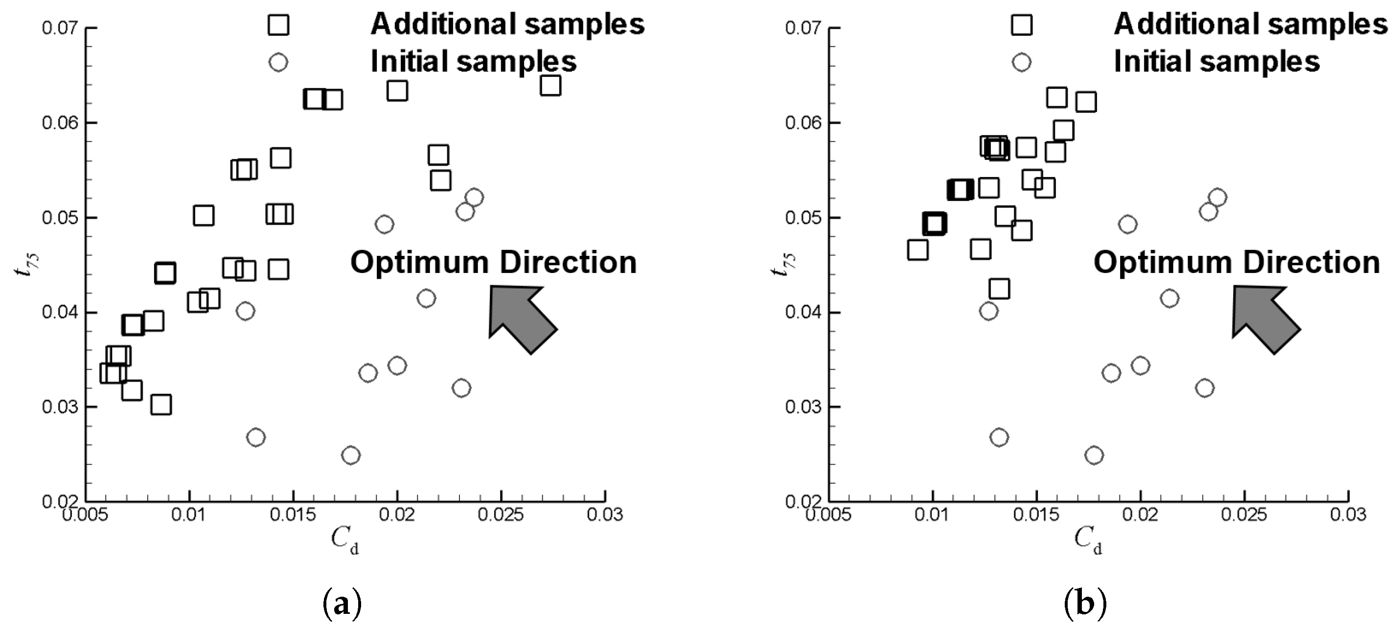
All the samples obtained by the two methods (the proposed multi-fidelity/multi-objective EGO and the single-fidelity/multi-objective EGO) are shown in Figure 11. These results show that the proposed multi-fidelity/multi-objective EGO can achieve greater diversity in the solution space than the single-fidelity/multi-objective EGO. The hypervolume of the proposed multi-fidelity/multi-objective EGO showed faster convergence (after 20 iterations) than that of the single-fidelity/multi-objective EGO (after 26 iterations). In addition, the non-dominated solutions of the proposed multi-fidelity/multi-objective EGO included $C_{\mathrm{d}}$ ranging from 0.006 to 0.027 and $t_{75}$ ranging from 0.034 to 0.064. On the other hand, the non-dominated solutions of the single-fidelity/multi-objective EGO included $C_{\mathrm{d}}$ ranging from 0.009 to 0.016 and $t_{75}$ ranging from 0.047 to 0.064. The histories of the hypervolumes of the two methods are compared in Figure 12. According to these results, the single-fidelity surrogate model could find only local optimum points, whereas the proposed multi-fidelity approach could find global optimum points.

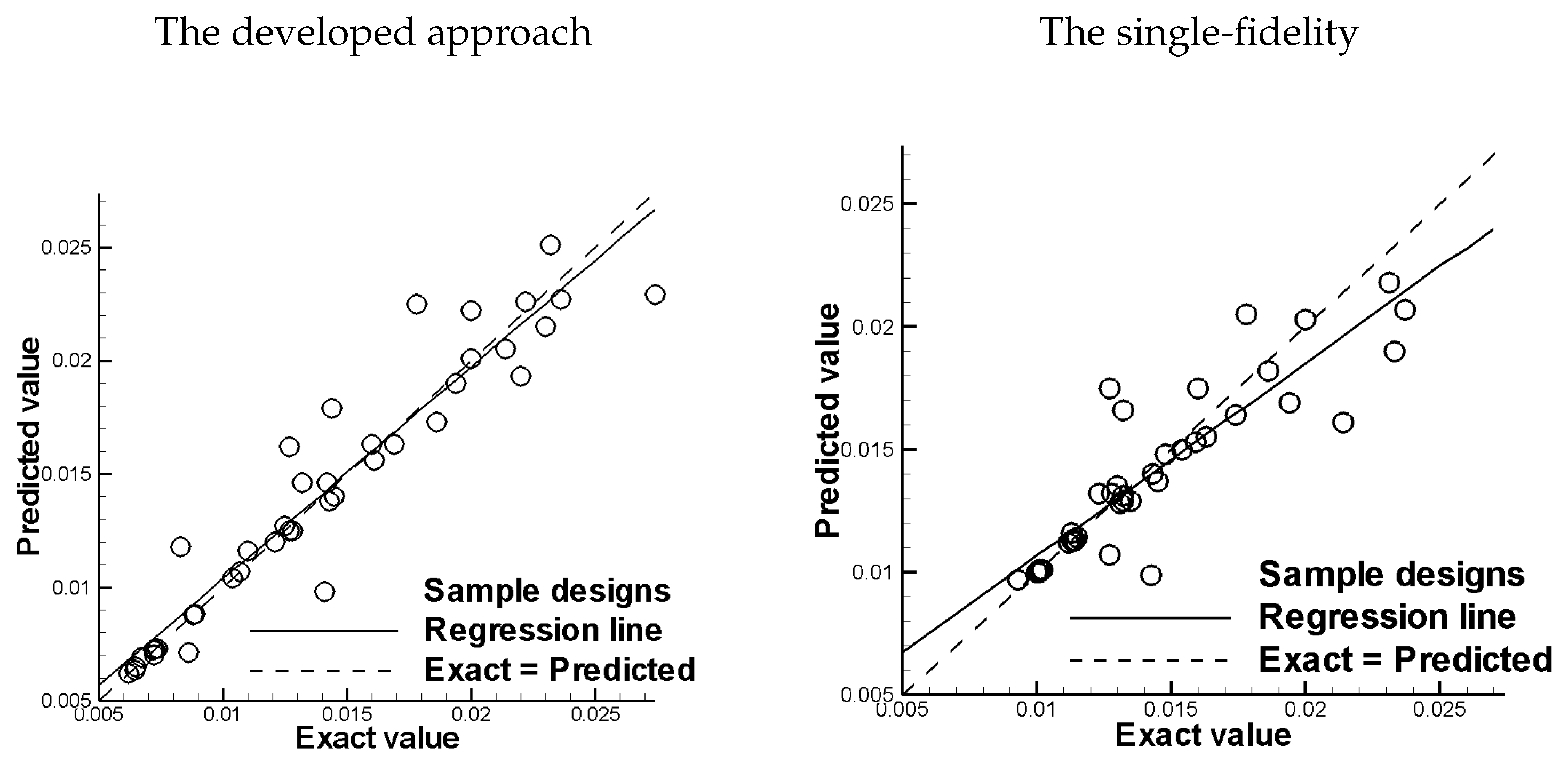
The cross-validation results for $C_{\mathrm{d}}$ are shown in Figure 13. It can be confirmed that the hybrid surrogate model achieves higher accuracy than the single-fidelity kriging-based surrogate model. This is because the low-fidelity data enable the surrogate model to predict the data in the uncertainty region. Thus, the multi-fidelity/multi-objective EGO achieves faster solution converge because the multi-fidelity surrogate model achieves higher accuracy than the single-fidelity surrogate model. Because the proposed multi-fidelity surrogate model achieves higher accuracy, the optimization process based on it is more likely to obtain global optimum points.

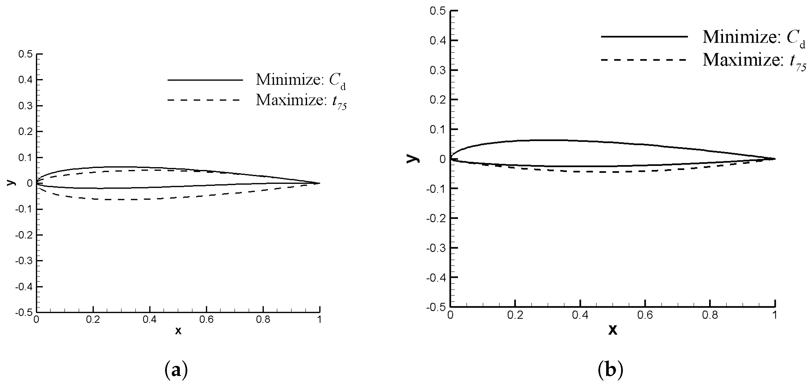
The optimal shapes of the non-dominated solutions of the two methods that minimize $C_{\mathrm{d}}$ and maximize $t_{75}$ are compared in Figure 14. The optimal designs of the single-fidelity/multi-objective EGO have similar shapes because the algorithm converges early at these optimum points. On the other hand, the optimal designs of the proposed multi-fidelity/multi-objective EGO have different shapes for each objective. In addition, the total design time of the multi-fidelity/multi-objective EGO is 162 min, and the total design time of the single-fidelity/multi-objective EGO is 160 min.

5.3.2. Three-Objective Airfoil Shape Optimization Results

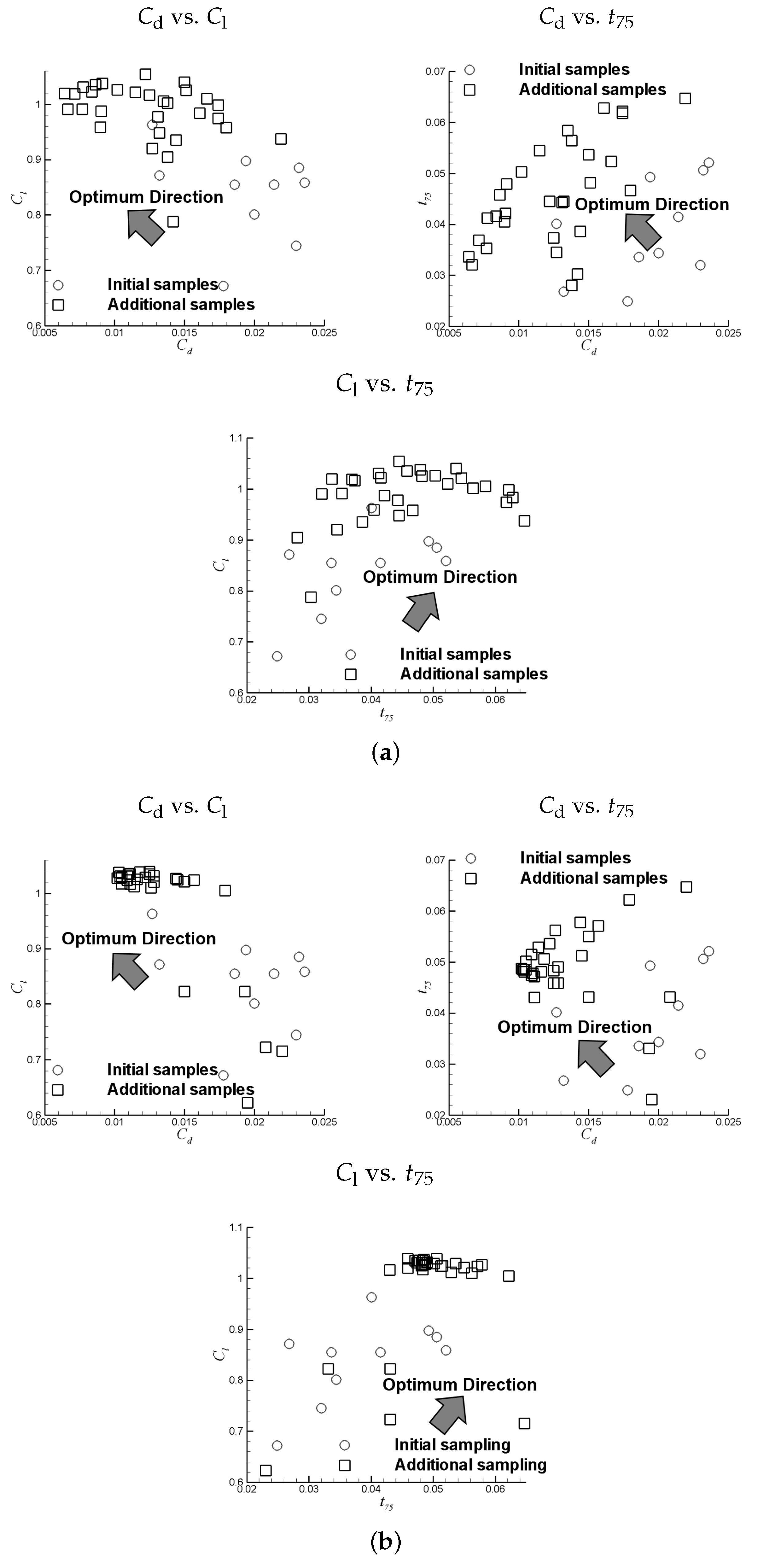
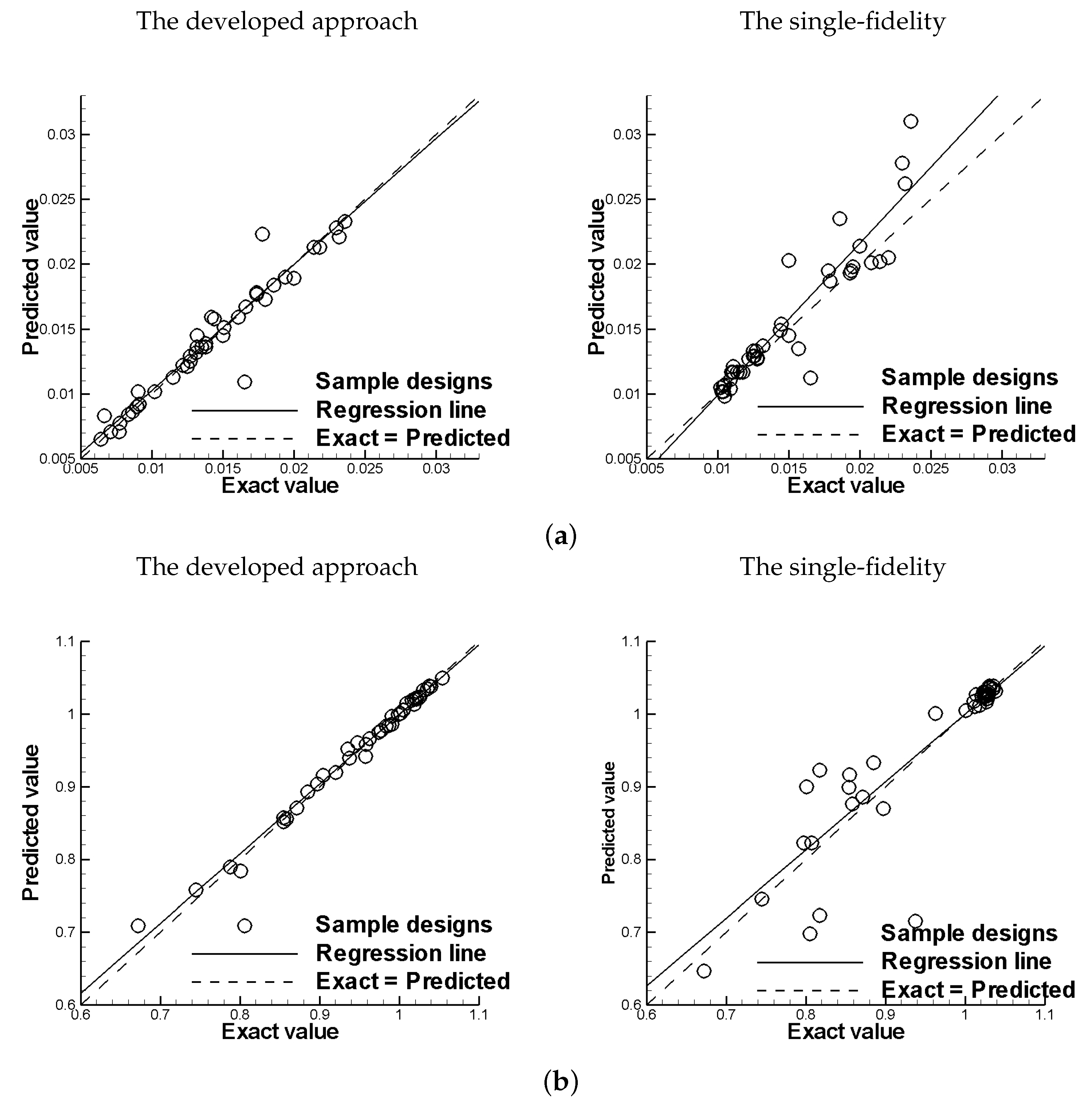
All the samples obtained by the two methods (the proposed multi-fidelity/multi-objective EGO and the single-fidelity/multi-objective EGO) are compared in Figure 15. In addition, the histories of the hypervolumes of the two methods are compared in Figure 16. These results show that the proposed multi-fidelity/multi-objective EGO achieves greater diversity of the non-dominated solutions because its hypervolume is larger than that of the single-fidelity/multi-objective EGO. The non-dominated solutions of the proposed multi-fidelity/multi-objective EGO included $C_{\mathrm{d}}$ ranging from 0.007 to 0.022, $t_{75}$ ranging from 0.034 to 0.065 and $C_{\mathrm{l}}$ ranging from 0.0938 to 1.054. On the other hand, the non-dominated solutions of the single-fidelity/multi-objective EGO included $C_{\mathrm{d}}$ ranging from 0.010 to 0.022, $t_{75}$ ranging from 0.047 to 0.065 and $C_{\mathrm{l}}$ ranging from 0.0938 to 1.039. Thus, the proposed multi-fidelity/multi-objective EGO achieved greater diversity of the solutions than the single-fidelity/multi-objective EGO. The cross-validation results for $C_{\mathrm{d}}$ and $C_{\mathrm{l}}$ are shown in Figure 17. It can be seen that the proposed hybrid surrogate model achieves higher accuracy than the single-fidelity kriging-based surrogate model. Thus, the proposed multi-fidelity/multi-objective EGO can achieve greater diversity of the solutions because its surrogate model achieves higher accuracy.

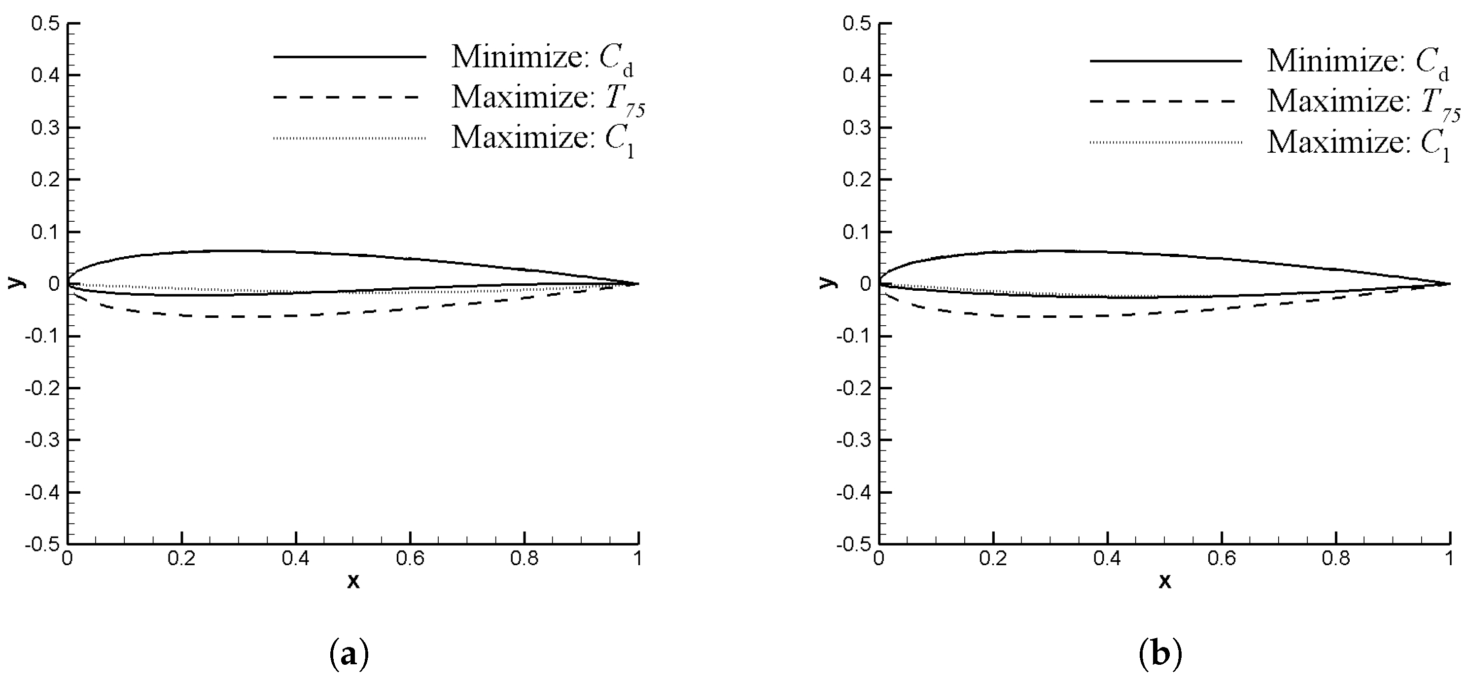
The optimal shapes of the non-dominated solutions of the two methods that minimize $C_{\mathrm{d}}$, maximize $t_{75}$ and maximize $C_{\mathrm{l}}$ are compared in Figure 18. The optimal designs of the single-fidelity/multi-objective EGO have similar shapes for minimizing $C_{\mathrm{d}}$ and maximizing $C_{\mathrm{l}}$ because the algorithm converges early at these optimum points. On the other hand, the optimal designs of the proposed multi-fidelity/multi-objective EGO have different shapes for each objective. In addition, the total design time of the multi-fidelity/multi-objective EGO is 162 min, and the total design time of the single-fidelity/multi-objective EGO is 160 min.

6. Conclusions

In this article, a multi-fidelity/multi-objective EGO combined with kriging and RBF was proposed based on the hybrid surrogate model to solve the multi-objective optimization problems and was applied to solve the multi-objective airfoil design problem. The proposed method constructed a hybrid surrogate model based on an RBF that predicts a global model and an ordinary kriging method that predicts the local variance. EHVI was used as an index to find additional samples for the optimization process. For multi-fidelity optimization, the global model was constructed using a dataset evaluated by a low-fidelity function, and the local variance was estimated using a dataset evaluated by a high-fidelity function.

To examine the proposed multi-fidelity/multi-objective EGO, two-/three-objective test problems were solved, and the results of the proposed multi-fidelity/multi-objective EGO were compared with those of the single-fidelity/multi-objective EGO. The results for the test functions showed that the proposed multi-fidelity/multi-objective EGO achieves faster convergence than the single-fidelity/multi-objective EGO. Moreover, the results showed that the proposed multi-fidelity/multi-objective EGO has greater diversity of the non-dominated solutions than the single-fidelity/multi-objective EGO. In addition, the results showed that the proposed multi-fidelity/multi-objective EGO has fewer global errors. Thus, the proposed multi-fidelity/multi-objective EGO can be widely applied to real-world problems.

Further, the proposed multi-fidelity/multi-objective EGO was applied to an aerodynamic airfoil shape optimization problem with two objectives: minimize $C_{\mathrm{d}}$ at cruising speed and maximize the thickness around the trialing edge. To evaluate the aerodynamic performance, XFOIL was used to construct a low-fidelity/low-cost dataset, and a Navier–Stokes solver was used to construct a high-fidelity/high-cost dataset. The results of the proposed multi-fidelity/multi-objective EGO were compared with those of the single-fidelity/multi-objective EGO. The optimization results showed that the proposed multi-fidelity/multi-objective EGO achieves greater diversity of the non-dominated solutions than the single-fidelity/multi-objective EGO. In addition, the cross-validation results showed that the proposed multi-fidelity/multi-objective EGO has fewer global errors. Finally, the proposed multi-fidelity/multi-objective EGO was applied to an aerodynamic airfoil shape optimization problem with three objectives: minimize $C_{\mathrm{d}}$ at cruising speed, maximize the thickness around the trialing edge and maximize $C_{\mathrm{l}}$ in the landing condition. The results showed that the proposed multi-fidelity/multi-objective EGO achieves greater diversity of the non-dominated solutions than the single-fidelity/multi-objective EGO. In addition, the error between the exact value and the predicted value of the hybrid surrogate model was smaller than that of the single-fidelity model. These results suggest that the multi-fidelity/multi-objective EGO is suitable for real-world multi-objective design problems. In this study, we limited the optimization to two/three objectives for simple aerodynamic design problems. In the future, we expect that our algorithm will be used to solve more complicated design problems, and we will investigate the effects of the application of multi-fidelity data in advanced kriging methods such as universal kriging and anisotropy kriging.

References

- Wickramasinghe, U.K.; Carrese, R.; Li, X. Designing airfoils using a reference point based evolutionary many-objective particle swarm optimization algorithm. IEEE Congr. Evolut. Comput. 2010, 10, 142–149. [Google Scholar]
- Ariyarit, A.; Kanazaki, M. Multi-modal distribution crossover method based on two crossing segments bounded by selected parents applied to multi-objective design optimization. J. Mech. Sci. Technol. 2015, 29, 1443–1448. [Google Scholar] [CrossRef]
- Choi, S.; Alonso, J.J.; Kroo, I.M. Two-level multifidelity design optimization studies for supersonic jets. J. Aircr. 2009, 46, 776–790. [Google Scholar] [CrossRef]
- Liu, W.-F.; Li, S.-Y.; Gong, Z.B.; Jiang, Z. Airfoil Optimization Design by Panel Methods for Small Size Aerial Vehicle at Low Reynolds Number. In Proceedings of the 1st International Conference on Mechanical Engineering and Material Science, Shanghai, China, 28–30 December 2012. [Google Scholar]
- Jameson, A. Optimum aerodynamic design using CFD and control theory. AIAA Paper 1995, 1729, 124–131. [Google Scholar]
- Choi, S.; Alonso, J.J.; Kroo, I.M.; Wintzer, M. Multifidelity design optimization of low-boom supersonic jets. J. Aircr. 2008, 46, 106–118. [Google Scholar] [CrossRef]
- Forrester, A.I.J.; Sobester, A.; Keane, A.J. Multi-fidelity optimization via surrogate modelling. Proc. R. Soc. Lond. A 2007, 463. [Google Scholar] [CrossRef]
- Huang, L.; Gao, Z.; Zhang, D. Research on multi-fidelity aerodynamic optimization methods. Chin. J. Aeronaut. 2013, 26, 279–286. [Google Scholar] [CrossRef]
- Khuri, A.I.; Mukhopadhyay, S. Response surface methodology. Wiley Interdiscip. Rev. 2010, 2, 128–149. [Google Scholar] [CrossRef]
- Rethore, P.E.; Fuglsang, P.; Larsen, G.C.; Buhl, T.; Larsen, T.J.; Madsen, H.A. TopFarm: Multi-fidelity optimization of offshore wind farm. In Proceedings of the Twenty-first International Offshore and Polar Engineering Conference, Maui, Hawaii, USA, 19–24 June 2011. [Google Scholar]
- Rethore, P.E.; Fuglsang, P.; Larsen, G.C.; Buhl, T.; Larsen, T.J.; Madsen, H.A. TopFarm: Multi-fidelity optimization of offshore wind farm. Wind Energy 2014, 17, 1797–1816. [Google Scholar] [CrossRef] [Green Version]
- Leon, E.R.; Le Pape, A.; Désidéri, J.A.; Alfano, D. Multi-Fidelity Concurrent Aerodynamic Optimization of Rotor Blades in Hover and Forward Flight. In Proceedings of the 40th European Rotorcraft Forum, Southampton, UK, 2–5 September 2014. [Google Scholar]
- Leusink, D.; Alfano, D.; Cinnella, P. Multi-fidelity optimization strategy for the industrial aerodynamic design of helicopter rotor blades. Aerosp. Sci. Technol. 2015, 42, 136–147. [Google Scholar] [CrossRef]
- Collins, K.B.; Sankar, L.N.; Mavris, D.N. Application of low-and high-fidelity simulation tools to helicopter rotor blade optimization. J. Am. Helicopter Soc. 2013, 58, 1–10. [Google Scholar]
- Fusi, F.; Guardone, A.; Quaranta, G.; Congedo, P.M. Multifidelity Physics-Based Method for Robust Optimization Applied to a Hovering Rotor Airfoil. AIAA J. 2015. [Google Scholar] [CrossRef]
- Jones, D.R.; Schonlau, M.; Welch, W.J. Efficient global optimization of expensive black-box functions. J. Glob. Optim. 1998, 13, 455–492. [Google Scholar] [CrossRef]
- Couckuyt, I.; Deschrijver, D.; Dhaene, T. Fast calculation of multiobjective probability of improvement and expected improvement criteria for Pareto optimization. J. Glob. Optim. 2014, 60, 575–594. [Google Scholar] [CrossRef]
- Hupkens, I.; Emmerich, M.; Deutz, A. Faster Computation of Expected Hypervolume Improvement. arXiv, 2014; arXiv:1408.7114. [Google Scholar]
- Orr, M.J.L. Introduction to Radial Basis Function Networks; Institute for Adaptive and Neural Computation, Edinburgh University: Edinburgh, UK, 1996. [Google Scholar]
- Praveen, C.; Duvigneau, R. Radial basis functions and kriging metamodels for aerodynamic optimization; RapiTech: Shanghai, China, 2007; Volume 159. [Google Scholar]
- Matheron, G. Principles of geostatistics. Econ. Geol. 1963, 58, 1246–1266. [Google Scholar] [CrossRef]
- Moore, R. Geostatistics in Hydrology: Kriging Interpolation; Technical Report; Mathematics Department, Macquarie University: Sydney, Australia, 1999. [Google Scholar]
- Goldberg, D.E.; Holland, J.H. Genetic algorithms and machine learning. Mach. Learn. 1988, 3, 95–99. [Google Scholar] [CrossRef]
- Bader, J.; Zitzler, E. HypE: An algorithm for fast hypervolume-based many-objective optimization. Evolut. Comput. 2011, 19, 45–76. [Google Scholar] [CrossRef] [PubMed]
- Everson, R.M.; Fieldsend, J.E.; Singh, S. Full elite sets for multi-objective optimisation. In Adaptive Computing in Design and Manufacture V; Springer: London, UK, 2002; pp. 343–354. [Google Scholar]
- Eshelman, L.J. Real-Coded Genetic Algorithms and Interval-Schemata. In Foundations of Genetic Algorithms; Elsevier: Amsterdam, The Netherlands, 1993; pp. 187–202. [Google Scholar]
- Melanie, M. The title of the cited contribution. In An Introduction to Genetic Algorithms; Publishing House: Cambridge, MA, USA, 1999; pp. 62–75. [Google Scholar]
- Huband, S.; Hingston, P.; Barone, L.; While, L. A review of multiobjective test problems and a scalable test problem toolkit. IEEE Trans. Evol. Comput. 2006, 10, 477–506. [Google Scholar] [CrossRef]
- Liem, R.P.; Mader, C.A.; Martins, J.R.R.A. Surrogate models and mixtures of experts in aerodynamic performance prediction for aircraft mission analysis. Aerosp. Sci. Technol. 2015, 43, 126–151. [Google Scholar] [CrossRef]
- Meckesheimer, M.; Booker, A.J.; Barton, R.R.; Simpson, T.W. Computationally inexpensive metamodel assessment strategies. AIAA J. 2002, 40.10, 2053–2060. [Google Scholar] [CrossRef]
- Obayashi, S.; Guruswamy, G.P. Convergence acceleration of a Navier–Stokes solver for efficient static aeroelastic computations. AIAA J. 1995, 33, 1134–1141. [Google Scholar]
- Yoon, S.; Jameson, A. Lower-upper symmetric-Gauss-Seidel method for the Euler and Navier–Stokes equations. AIAA J. 1988, 26, 1025–1026. [Google Scholar] [CrossRef]
- Fujii, K.; Obayashi, S. High-resolution upwind scheme for vortical-flow simulations. J. Aircr. 1989, 26, 1123–1129. [Google Scholar] [CrossRef]
- Baldwin, B.S.; Barth, T.J. A One-Equation Turbulence Transport Model for High Reynolds Number Wall-Bounded Flows; NASA: Washington, DC, USA, 1990. [Google Scholar] [CrossRef]
- Drela, M. XFOIL: An analysis and design system for low Reynolds number airfoils. In Low Reynolds Number Aerodynamics; Springer: Berlin/Heidelberg, Germany, 1989; pp. 1–12. [Google Scholar]
- Kulfan, B.M. Universal parametric geometry representation method. J. Aircr. 2008, 45, 142–158. [Google Scholar] [CrossRef]
- Lorentz, G.G. Bernstein Polynomials; American Mathematical Society: Providence, RI, USA, 2012. [Google Scholar]
Figure 1.
Schematic illustration of single-fidelity and multi-fidelity surrogate models.
Figure 2.
Flowchart of efficient global optimization: (a) single-fidelity efficient global optimization (EGO); (b) multi-fidelity EGO.
Figure 3.
Schematic illustration of hypervolume improvement and hypervolume: (a) hypervolume improvement; (b) hypervolume.
Figure 4.
Initial sampling data and additional sampling data of two-objective test problem: (a) multi-fidelity approach; (b) single-fidelity approach.
Figure 5.
Hypervolume comparison of multi-fidelity approach and single-fidelity approach of two-objective test problem.
Figure 6.
Cross-validation results of the two-objective test problem: (a) result of ; (b) result of .
Figure 7.
Initial sampling data and additional sampling data of three-objective test problem: (a) multi-fidelity approach; (b) single-fidelity approach.
Figure 8.
Hypervolume comparison of the multi-fidelity approach and the single-fidelity approach of three-objective test problem.
Figure 9.
Cross-validation results of the three-objective test problem: (a) result of ; (b) result of ; (c) result of .
Figure 10.
Computation structured grid: (a) full length; (b) grid around the airfoil.
Figure 11.
Initial sampling data and additional sampling data of two-objective airfoil shape optimization problem: (a) multi-fidelity approach; (b) single-fidelity approach.
Figure 12.
Hypervolume comparison of multi-fidelity approach and single-fidelity approach of two-objective airfoil shape optimization problem.
Figure 13.
Cross-validation of two-objective airfoil shape optimization problem of .
Figure 14.
Comparison of design geometries of two-objective airfoil shape optimization problem: (a) multi-fidelity approach; (b) single-fidelity approach.
Figure 15.
Initial sampling data and additional sampling data of three-objective airfoil shape optimization problem: (a) multi-fidelity approach; (b) single-fidelity approach.
Figure 16.
Hypervolume comparison of multi-fidelity approach and single-fidelity approach.
Figure 17.
Cross-validation results of three-objective airfoil shape optimization problem: (a) results of ; (b) results of .
Figure 18.
Comparison of design geometries of three-objective airfoil shape optimization problem: (a) multi-fidelity approach; (b) single-fidelity approach.