An Accurate Perception Method for Low Contrast Bright Field Microscopy in Heterogeneous Microenvironments ^†

Abstract

Automated optical tweezers-based robotic manipulation of microscale objects requires real-time visual perception for estimating the states, i.e., positions and orientations, of the objects. Such visual perception is particularly challenging in heterogeneous environments comprising mixtures of biological and colloidal objects, such as cells and microspheres, when the popular imaging modality of low contrast bright field microscopy is used. In this paper, we present an accurate method to address this challenge. Our method combines many well-established image processing techniques such as blob detection, histogram equalization, erosion, and dilation with a convolutional neural network in a novel manner. We demonstrate the effectiveness of our processing pipeline in perceiving objects of both regular and irregular shapes in heterogeneous microenvironments of varying compositions. The neural network, in particular, helps in distinguishing the individual microspheres present in dense clusters.

1. Introduction

Optical tweezers (OT) are well-suited for contact free manipulation of microscale objects of various shapes, dimensions and material compositions [1]. It uses a high numerical aperture microscope objective to tightly focus a laser beam that exerts the required amount of force to grasp (trap), move and orient microscale objects in a fluid medium. A large number of microscale objects are manipulated simultaneously by using a dynamic hologram to split the beam into multiple beams with complete individual control over the focal positions of each of the beams in three dimensions [2]. Combining these characteristics with low trapping force magnitudes (tens of picoNewtons) and the dependence of the forces on the relative refractive index of the manipulated objects with respect to the surrounding medium, the OT system is used often in many biomanipulation applications such as cell sorting, drug delivery and mechanistic study of fundamental physiological processes [3].

By automating the process of controlling the laser beams, the OT functions as an optically actuated microrobot with multiple reconfigurable end effectors (see Figure 1), or a collection of independently steerable microrobots [4]. We are particularly interested in the indirect manipulation of a large number of cells to study their collective migration behaviors in the presence of external stimuli or form precise patterns such as vascular microstructures that can be embedded within maturing engineered tissue constructs. These cells are not trapped directly by the laser beams to avoid photodamage caused by laser exposure induced local heating or photopolymerization. Instead, they are manipulated by inert end effectors, which consist of optically-trapped microspheres (beads) that are completely unaffected by the laser [5]. The trapped beads are able to easily grasp as well as release the cells due to the absence of chemical bonding or functional adhesion between the beads and the cells.

Such automated micromanipulation requires accurate, real-time estimation of the positions and orientations (states) of the workspace objects. These estimated states are combined with a dynamical model of the objects, and fed to a path planner to compute collision-free object trajectories. Trajectory information is then provided to a motion controller to execute stable actions (set and change the focal positions of the laser beams) that closely follow the trajectories. Considering that the objects are sensed using a charge-coupled device (CCD) camera employing standard bright field imaging, being able to process the low contrast images to perceive what type of object is located where is important. Since some of the objects change shape dynamically, it is necessary for any perception method to track object boundaries in addition to detecting their centroid locations and motion directions. It is also important for the perception method to work in a variety of fluid media offering different background image contrasts where the objects will be manipulated.

A plethora of work already exists in the context of automated optical micromanipulation, particularly for dynamics modeling, path planning and motion control. Representative examples of dynamics modeling include the use of Langevin equation to simulate the behavior of an optically-trapped microsphere [6] and a stochastic perturbation model to analyze the trapping stability of microparticles during motion [7]. For path or trajectory planning, representative examples include a partially observable Markov decision process algorithm for single object [8] and multiple object [9] transport, a rapidly-exploring random tree method for cell transport [10], and an A* algorithm for indirect manipulation of cells using optically-trapped microspheres [11]. With respect to motion control, recent representative works include a vision-based observer method for multiple cell transport [12], a proportional-derivative (PD) control strategy for single cell transport [13], a saturation controller for swarming motions of cells [14], a combined translational and rotational controller for cells [15], and a motorized stage-optical tweezers cooperative controller for multi-cell manipulation [16]. Other representative methods include a disturbance compensation controller for in vivo cell manipulation [17], a potential field controller for multi-stage cell transport [18], a neural network controller for object manipulation in the presence of unknown optical trapping stiffness [19], a model predictive controller for microsphere pattern formation [20,21], and independent actuation of fifty microrobots using optically generated thermal gradients [22].

Magnetic actuation provides an alternative technique for automated biomanipulation that has attracted a lot of attention. Magnetic manipulation involves either using time varying magnetic fields to move the biological objects directly [23,24], or using time varying magnetic fields to move microrobots that serve as end effectors for the objects [25,26,27,28,29]. We refer the interested reader to [30] for a survey of automated planning and control methods across different micromanipulation techniques, to [31] for a recent review of the advances in controlling multiple microrobots, and to [32] for a discussion on various designs of magnetically actuated microrobots. However, as in the case of optical manipulation, not much work has been done to specifically address the problem of microscale object perception from bright field imaging.

While there are a handful of methods for bright field image processing, most of them require a set of defocused images at varying heights and/or detect objects of one type only [33,34,35,36]. Moreover, some of the methods are not suitable for real-time implementation [37] or only work for specific cell shapes [38]. We have developed a method to address many of these limitations and perceive objects of varying types and shapes from a series of time-lapse images taken at the same cross-sectional plane [39]. Our method is based on a novel combination of many well-known image processing techniques. Here, we further demonstrate the effectiveness of the method in providing highly accurate and precise perception results for multiple cell types, including human cells, in different fluid media, whose compositions may vary over time. In addition, we present a convolutional neural network model to distinguish the individual beads even in tightly aggregated clusters.

2. Materials and Methods

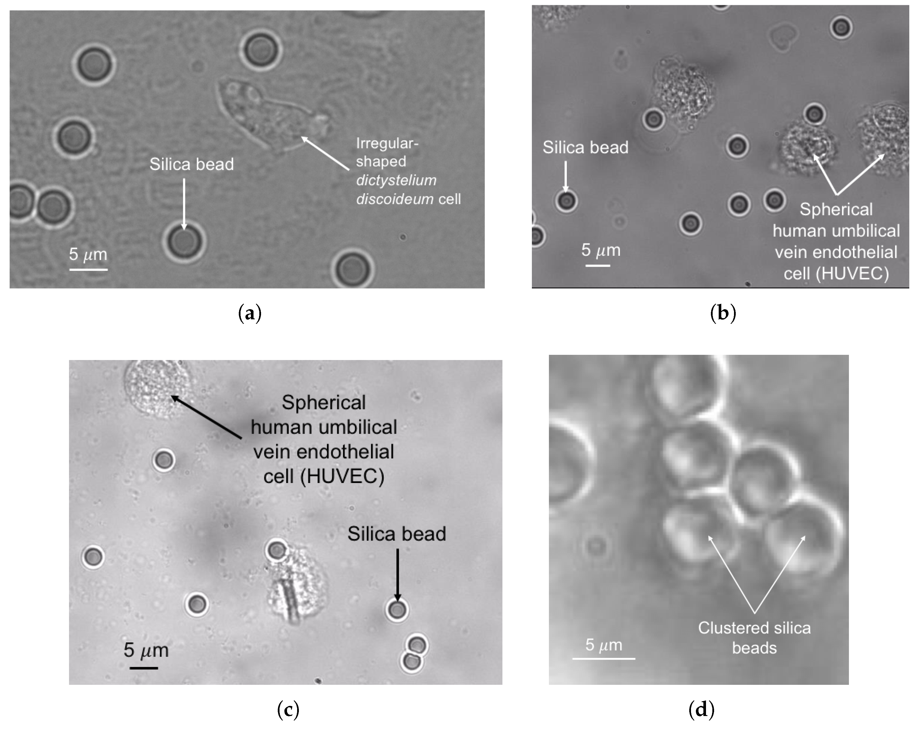
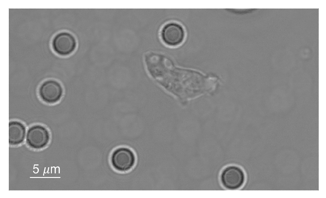
2.1. Data

Four distinct sequences of images are used to develop an accurate microscale object perception method. The first sequence of images, $I^{iw}(x,y)=\{I_1^{iw}(x,y),\dots ,I_{N_1}^{iw}(x,y)\}$, contains microspheres (beads) and irregular-shaped amoeba cells suspended in water. Note that the shapes of the amoeba cells change dynamically following a wave-like pattern with a leading side and a trailing side as they move around in the medium. Each image is represented as a matrix of gray scale intensity values at every $(x,y)$ pixel location. The second sequence of images, $I^{sw}(x,y)=\{I_1^{sw}(x,y),\dots ,I_{N_2}^{sw}(x,y)\}$, contains beads and regular-shaped (mostly spherical) human endothelial cells (hECs) dispersed in water. The third sequence of images, $I^{sm}(x,y)=\{I_1^{sm}(x,y),\dots ,I_{N_3}^{sm}(x,y)\}$, contains beads and hECs in Matrigel, a commonly used extracellular matrix for cell culture and engineered tissue development. It is worth pointing out that the composition of Matrigel changes spontaneously during cell manipulation at room temperature due to polymerization or gel formation. This change in composition alters the background contrast of the bright field images. The fourth sequence of images, $I^{cm}(x,y)=\{I_1^{cm}(x,y),\dots ,I_{N_4}^{cm}(x,y)\}$, comprises dense aggregates (clusters) of beads in Matrigel. Example images from all the sequences are shown in Figure 2.

$I^{iw}(x,y)$, $I^{sw}(x,y)$, $I^{sm}(x,y)$, and $I^{cm}(x,y)$ are provided as inputs to the perception method. The method first categorizes an imaged object to be either a bead or a cell. It then computes the centroids and diameters of the beads, and the centers, dimensions and orientations (with respect to the horizontal axis) of the bounding boxes for the cells. It also traces the beads boundaries and the cells contours. For the objects that are present along the image boundaries and are only partially visible, the method does not attempt to categorize them into any type, but still computes their centroids and traces their boundaries. We describe the method in detail in the next sub-Section, and use $I_j^{iw}(x,y)$, $I_j^{sw}(x,y)$, $I_j^{sm}(x,y)$, and $I_j^{cm}(x,y)$ as examples to illustrate the result of each method step.

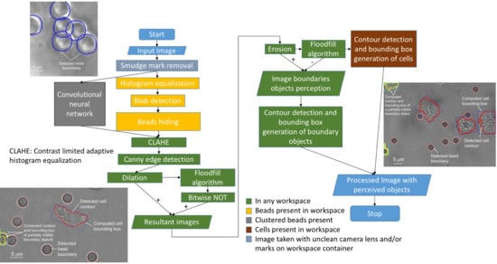
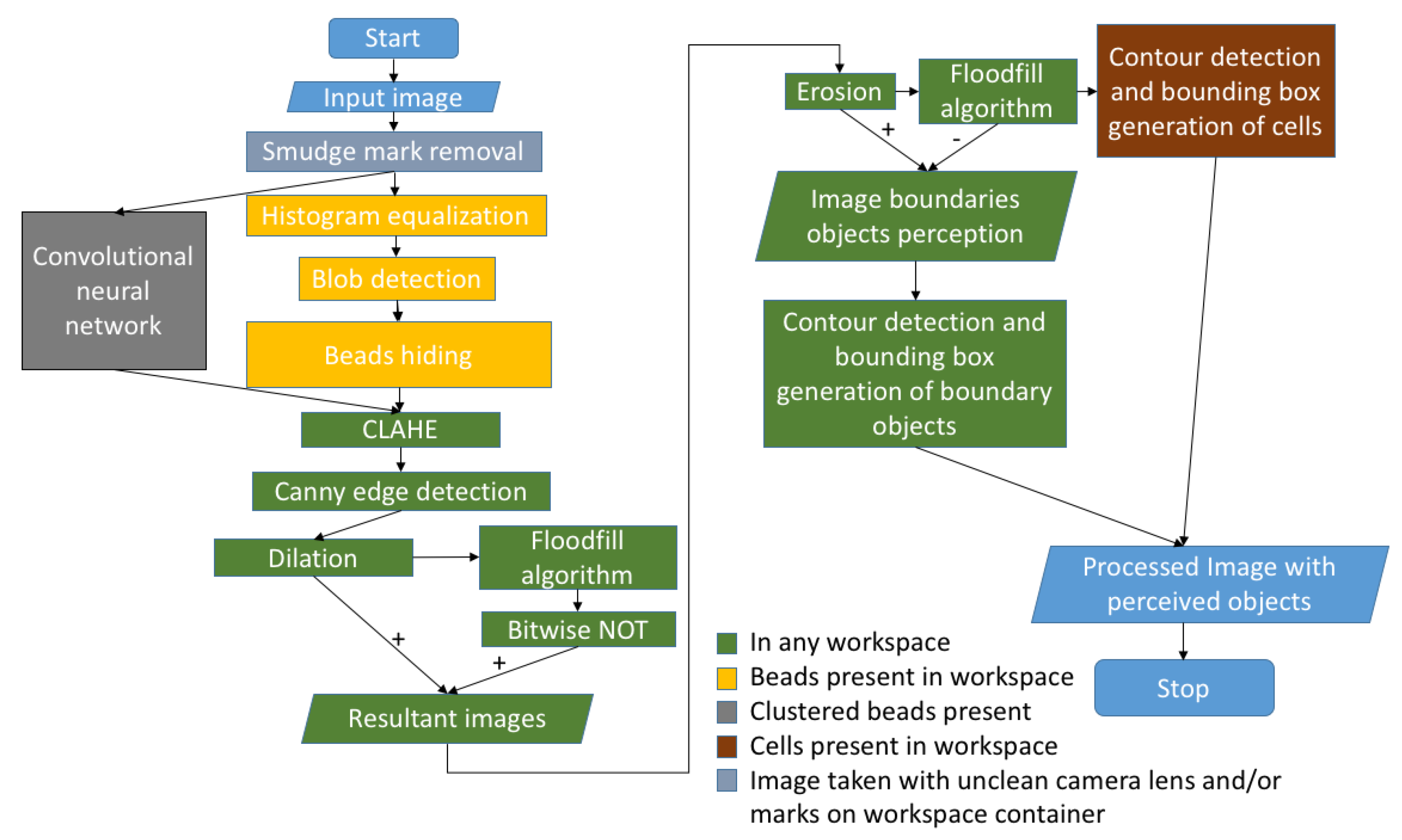
2.2. Technical Approach

The object perception algorithm consists of three main steps: (1) smudge mark removal from the images (if necessary), (2) bead perception, including distinguishing the individual beads in clusters, and (3) cell perception, including detecting the partially visible objects.

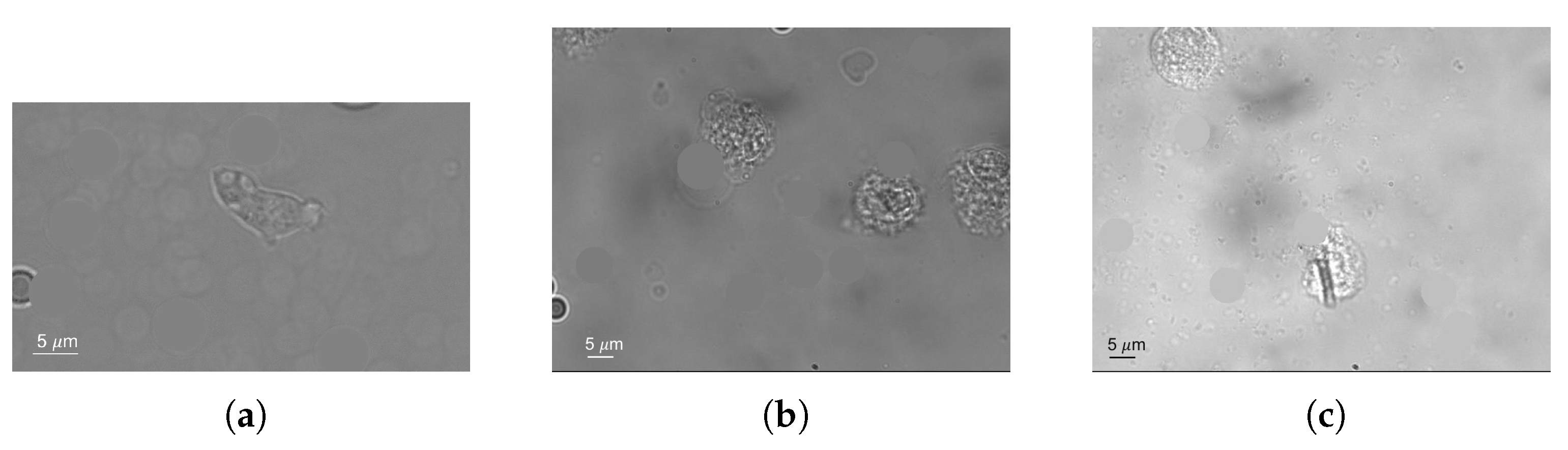
2.2.1. Smudge Mark Removal

We observe that the $I^{iw}(x,y)$ image has a pattern of smudge marks, which makes it difficult to accurately perceive the beads and cells present in the image. These smudge marks arise from an unclean camera lens and/or spillage of oil from the oil-immersion objective on the workspace container, which can be either a glass microscope slide or a glass-bottomed Petri dish. Such smudge marks are, however, not observed in the other images, $I^{sw}(x,y)$, $I^{sm}(x,y)$ and $I^{cm}(x,y)$. If such marks are present, we use an algorithm [40], which has been successful for outdoor robotics and computer vision applications, to remove the marks. The algorithm uses the following equation:

$$I_r(x,y)=\frac{I_o(x,y)-cb(x,y)}{a(x,y)},$$

(1)

where $I_r(x,y)$ denotes the smudge-free image; $I_o(x,y)\in I^{iw}(x,y)$ represents the original image; $a(x,y)$ is the attenuation map that models the reduction in illumination due to absorption by lens dirt; $b(x,y)$ is the intensification map that captures the scattering effect of lens dirt; and c is the aggregate of scene-dependent, outside illumination intensity. $a(x,y)$, $b(x,y)$ and c are then given as

$$a(x,y)=\frac{Avg\left(\right|\nabla I\left|\right)}{Avg\left(\right|\nabla I_{est}\left|\right)},$$

(2)

$$b(x,y)=Avg\left(I\right)-Avg\left(I_{est}\right)a(x,y),$$

(3)

$$c=\underset{c}{\arg \min }\left|\right|\nabla I_r(x,y){\left|\right|}_1.$$

(4)

Here, $Avg(.)$ denotes an averaging operation and I represents a set of training or calibration images of the same workspace using the same camera system but with some objects’ movements across the different image frames. $Avg\left(\right|\nabla I\left|\right)$ is the averaged magnitude of the image gradient over the calibration set, and $Avg\left(I_{est}\right)$ and $Avg\left(\right|\nabla I_{est}\left|\right)$ are estimated from $Avg\left(I\right)$ and $Avg\left(\right|\nabla I\left|\right)$, respectively, using least squares fitting with a bivariate polynomial ${\sum }_3^{i=0}{\sum }_3^{j=0}{a}_{ij}{x}^i{y}^j$, where x and y are normalized pixel coordinates. $a(x,y)$ and $b(x,y)$ are pre-computed from I, whereas c is calculated online for the first few images and the average of all the c values is used for the rest of the images as outside illumination remains the same. An example of a smudge-free image, $I_r^{iw}(x,y)$, is shown in Figure 3.

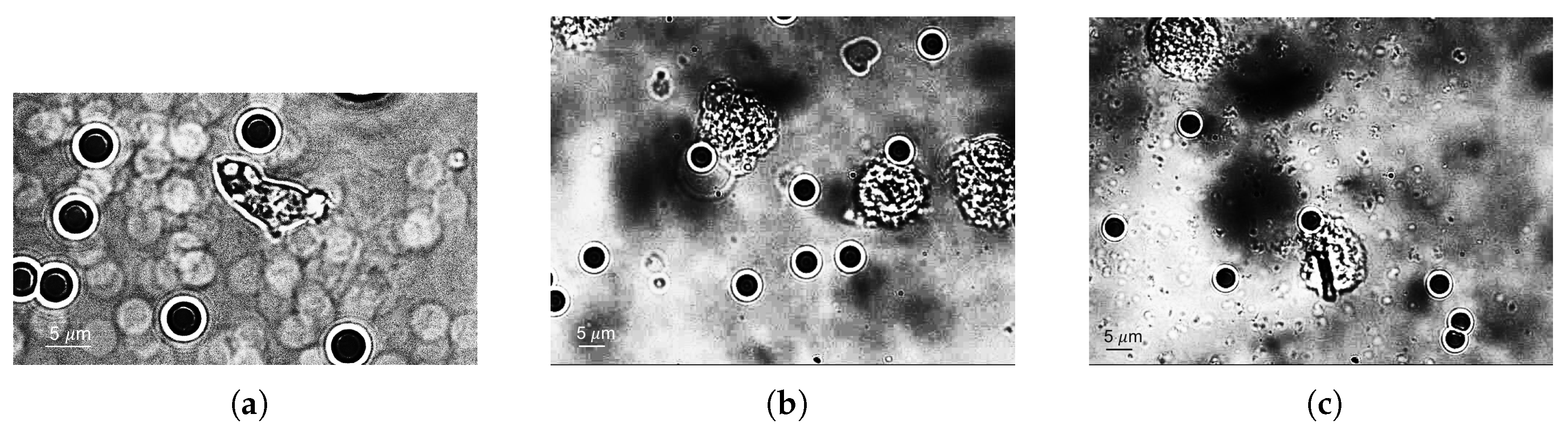
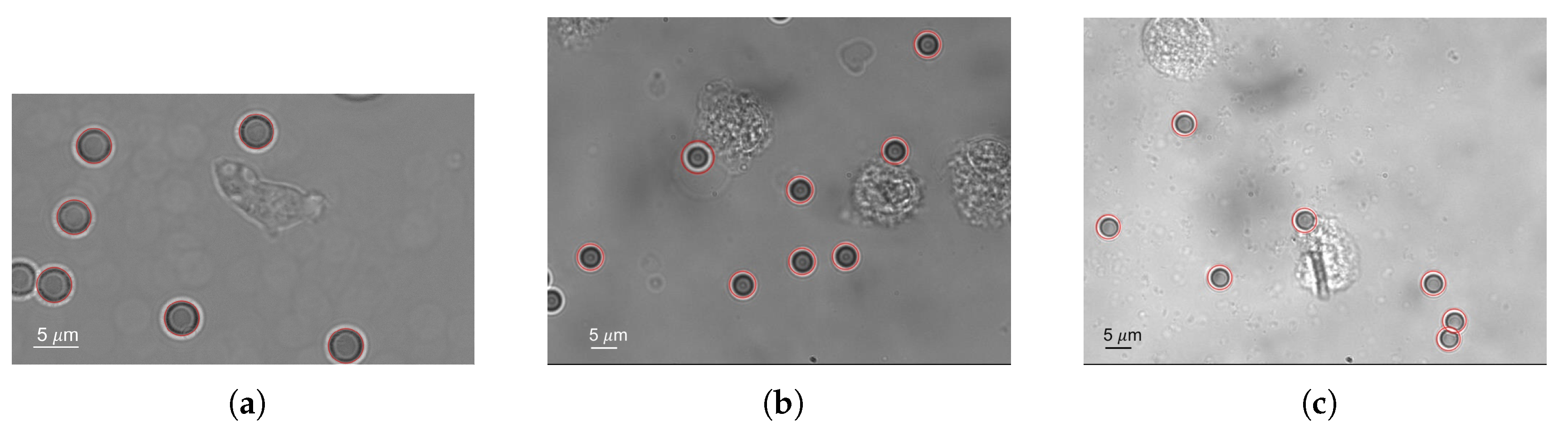
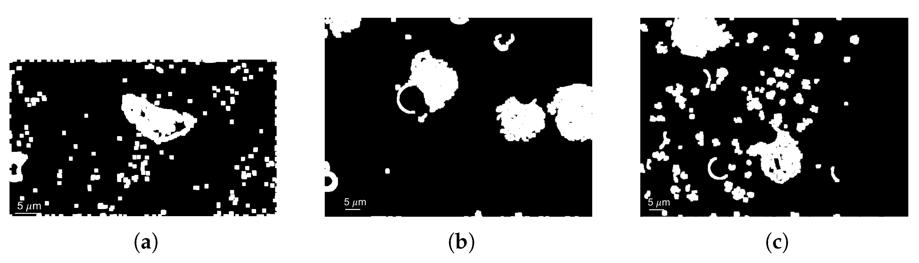
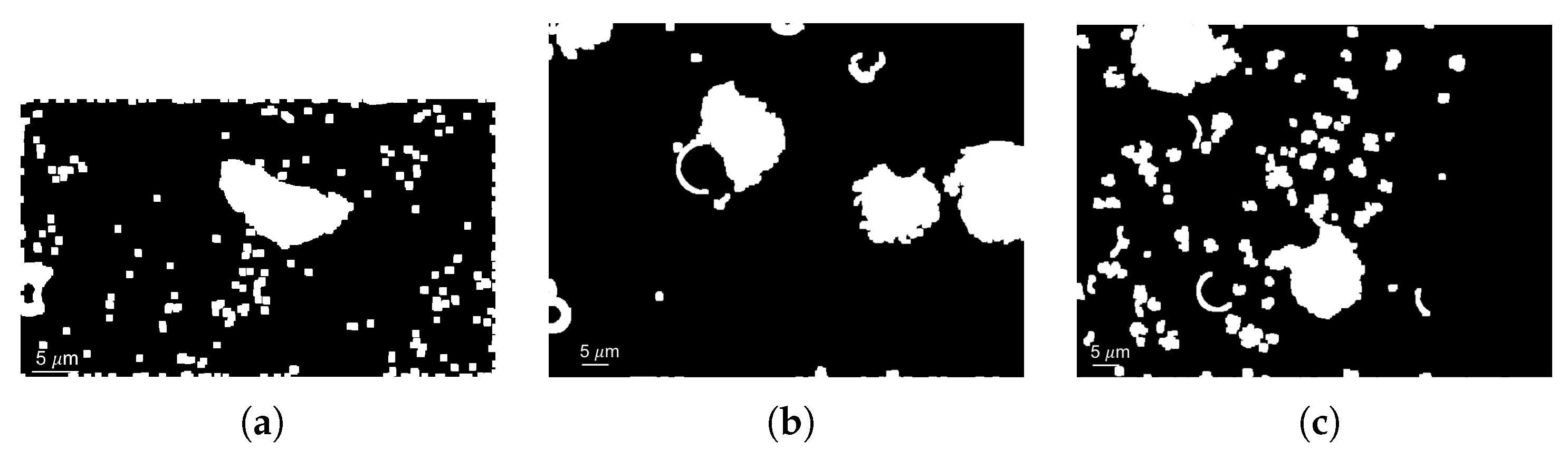
2.2.2. Bead Perception

We first apply the histogram equalization method (on either smudge-free or original images) to more equally distribute the intensity values across the images based on the intensities frequencies. This equalization improves the contrast of the locally low contrast regions of the image. The outcome of this method on $I_{jr}^{iw}(x,y)$, $I_{jr}^{sw}(x,y)$ and $I_{jr}^{sm}(x,y)$ to yield images $I_{jh}^{iw}(x,y)$, $I_{jh}^{sw}(x,y)$ and $I_{jh}^{sm}(x,y)$, respectively, is shown in Figure 4. Following this step, to reduce the noise without adversely affecting the contrast of the object edges, the median blurring method is applied. This blurring is done by replacing individual pixel intensities with the median intensity of the neighboring pixels that fall inside a user-specified kernel.

Observing that the beads possess similar properties such as area and intensity in all the the image sequences $I_r^{iw}(x,y)$, $I_r^{sw}(x,y)$ and $I_r^{sm}(x,y)$, we next use the blob detection method to identify the beads. In this method, the source image is first converted to multiple binary images by applying a binary thresholding for a set of evenly spaced thresholds. Contours of connected components are then found in each of these binary images using a topological border following algorithm [41]. The centers of the connected components are computed, and they are grouped together on the basis of their closeness (parametric distance) to each other. Every such group is designated as a blob, and the overall blob centers and radii are recorded. One challenge here is that this method compares the properties of the blobs with those of their surroundings for detection. As the image boundary objects do not have surrounding pixels on all the sides for comparison purposes, white boundaries are added to the median blurred images. The spherical cells are not identified as they do not qualify as blobs owing to irregularities in their intensities. The detected blobs are drawn on a copy of each image, and are represented as $I_b^{iw}(x,y)$, $I_b^{sw}(x,y)$ and $I_b^{sm}(x,y)$. Example images with identified beads are shown in Figure 5.

Convolutional Neural Network:

Though the above method works well in detecting separated beads, it encounters challenges when aggregates or clusters of beads are present in the fluid medium. To identify the individual beads in these clusters, i.e., perform segmentation, we use a convolutional neural net (CNN). CNNs have been shown to perform well in various image classification tasks [42]. Image segmentation can be performed by a fully CNN based encoder decoder system [43]. CNNs have also been successfully used in classifying complex datasets such as hand-written numbers [44].

To solve the problem of segmenting the clusters, we use pixel classification. Since we cannot be sure of the number of beads in any cluster, it is not feasible to predict the coordinates of the beads. The pixel classification approach helps us tackle this issue. Each pixel in an image is either classified as a bead center or not a bead center. The image is first padded by black spaces and then split into smaller images of size 31 × 31. Each of these sub images is centered on the pixel from the padded image. These sub images are then used as inputs to the CNN shown in Figure 6. The CNN architecture is modeled after the architecture presented in [44]. Both of the convolution layers are equipped with a commonly-used rectified linear unit (ReLU) activation function. This activation function helps to model nonlinearity in the output of each neuron w.r.t. the input x as shown in the equation below:

$$f\left(x\right)=max(0,x).$$

(5)

The first convolution layer has seven 7 × 7 filters. Filters are an array of weights, whose distribution enables the CNN to model any feature. The first layer also has a stride of 2, which means that the filters are applied by centering them on every other pixel in the input images. The second convolution layer has three filters of size 3 × 3 with stride equal to 1, meaning that the filters are applied on every pixel. The convolution layers are both followed by a max pooling layer of size 2 × 2. The max pooling layers help prevent over fitting in the CNN by downsampling, which is achieved by selecting the maximum value locally in a 2 × 2 grid from the output of the previous layer.

The final two layers in the CNN architecture are dense or fully connected layers, where all the inputs are connected to all the outputs. The first dense layer is of size 64 with the ReLU activation function. Since we are trying to classify if a pixel is a bead center or not, the final output of the network needs to be its confidence on these two mutually exclusive events. Hence, the final layer of the CNN is a dense layer of size 2 with a Softmax activation function shown in Equation (6). This activation function provides a probability distribution over the outputs in a layer. The actual sizes of the all the layers except the last one are found by trying different sizes and comparing their respective performances. After the CNN predicts the pixel states, those identified as bead centers are averaged with similarly classified neighboring pixels in a 3 × 3 grid:

$$\sigma \left(x\right)=\frac{\exp \left(x_i\right)}{{\displaystyle \sum _{i=1}^n}\exp \left(x_j\right).}$$

(6)

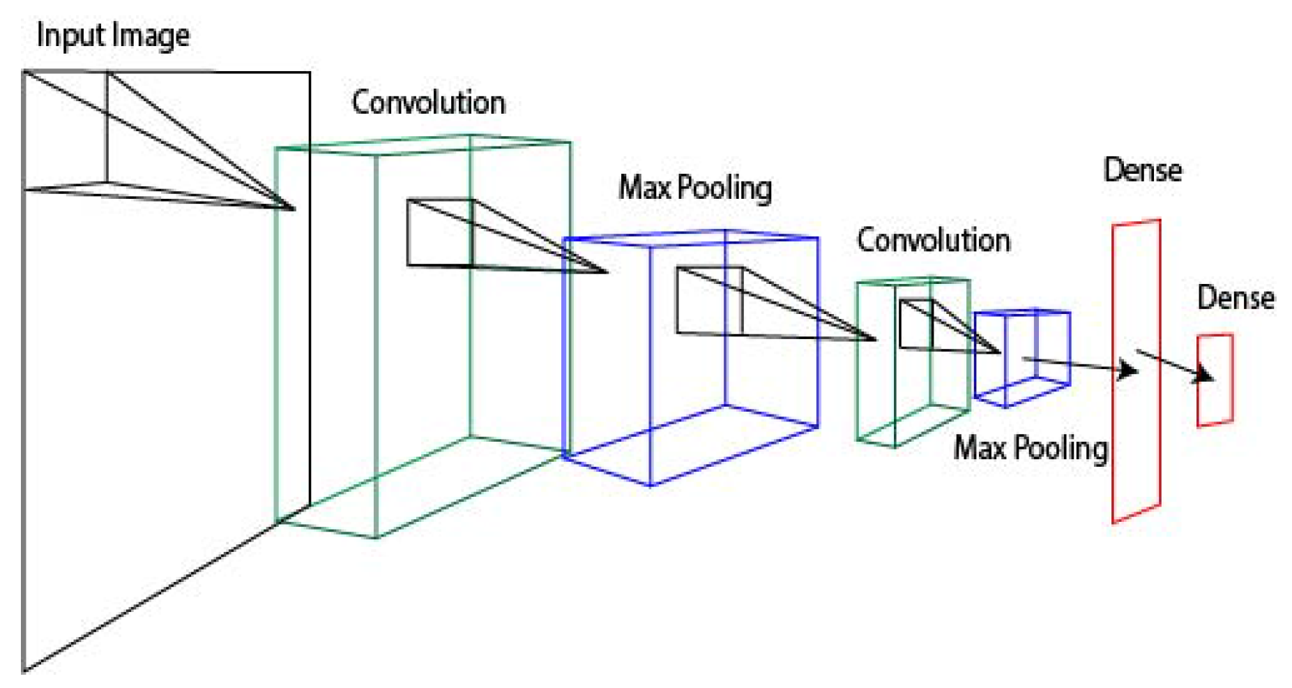
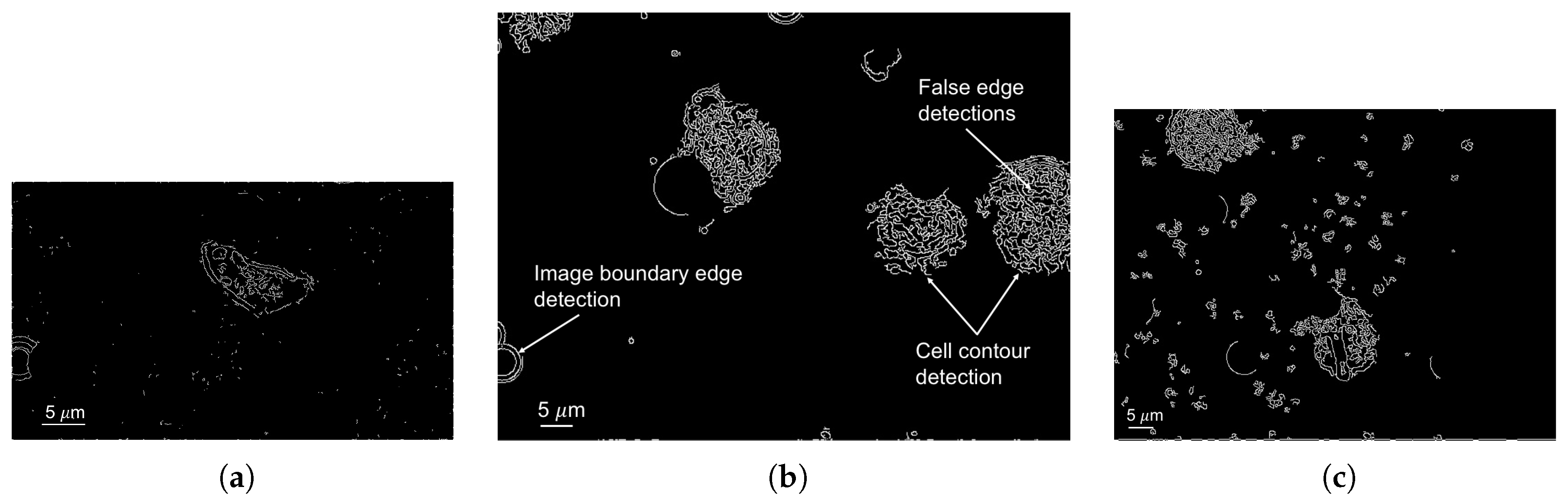
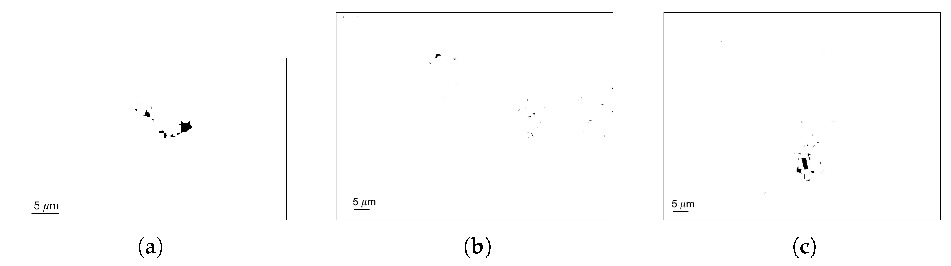
2.2.3. Cell Perception

We next address the task of perceiving the cells on the images where the beads are already identified. To do so, we first hide the identified beads by drawing appropriately sized-circles on top of the beads using the background image intensity, which is computed as the dominant pixel value from the image intensity histogram. The new images are denoted as $I_{bh}^{iw}(x,y)$, $I_{bh}^{sw}(x,y)$ and $I_{bh}^{sm}(x,y)$ for irregular-shaped amoeba cells in water and spherical human cells in water and Matrigel, respectively. They are shown in Figure 7. We then employ a sequence of steps to trace the contours and generate the bounding boxes for the cells. These steps are described as follows.

Edge detection:

We first want to detect the edges of the cells in the bright field images. For this purpose, we employ two well-known methods, namely, contrast limited adaptive histogram equalization (CLAHE) and Canny edge detection, one after the other. The CLAHE method partitions an image into small regions called tiles, where each tile’s contrast is enhanced using a combination of adaptive histogram equalization and a clipping algorithm [45]. The neighboring tiles are then merged using bilinear interpolation. Canny edge detector is a multi-step algorithm that detects a wide range of edges in images [46] by defining the edges as curved line segments comprising points of abrupt changes in image brightness. The processed binary image sets are denoted as $I_e^{iw}(x,y)$, $I_e^{sw}(x,y)$ and $I_e^{sm}(x,y)$, examples of which are shown in Figure 8. However, due to intensity variations in the interior regions and portions of the exterior regions of the cells, there are a large number of false detections. These false detections are handled by the subsequent steps of our perception method.

Dilation:

We now apply dilation on the binary images with detected edges. In this step, the foreground boundaries (i.e., the white pixels) are enlarged or dilated, where the amount of dilation depends on a user-specified kernel size and shape. The new processed images for our three data sets are denoted by $I_d^{iw}(x,y)$, $I_d^{sw}(x,y)$ and $I_d^{sm}(x,y)$, respectively, where the cells start to get filled up as seen in Figure 9. However, the number of white pixels in the cells exterior regions increase significantly even though a major portion of the cells’ interior regions turn white. Moreover, a small number of black pixels are still observed in the interior regions, which hinders accurate cell contour detection and needs to be taken care of.

Floodfill algorithm:

We now address the issue of detecting the disconnected black pixels in the cells interior regions. To do so, we first use the well-known floodfill algorithm. This algorithm requires two inputs, namely, a set of seed points and a replacement color. The pixels that are connected to the first seed point and have the same color as the seed point are filled by the replacement color, and this process is repeated for all the seed points one by one. We provide the image boundaries as the seed points and use white as the replacement color. Thus, this algorithm converts all the black pixels connected to the image boundaries to white. After employing this step on the dilated images, we obtain new binary images that are denoted by $I_f^{iw}(x,y)$, $I_f^{sw}(x,y)$ and $I_f^{sm}(x,y)$, respectively, examples of which are shown in Figure 10. We then use the bitwise NOT operation to convert all the white pixels to black and vice versa. This process is applied to the floodfilled images, and the resultant images, $I_{fd}^{iw}(x,y)$, $I_{fd}^{sw}(x,y)$ and $I_{fd}^{sm}(x,y)$, are added to the respective dilated images. The net effect of these operations is illustrated in Figure 11, which removes the previously detected black pixels in the cells’ interior regions.

Erosion:

Erosion is next applied on the floodfilled and dilated image sets to restore the size of the cell silhouettes that are enlarged by dilation. This process is the opposite of dilation in the sense that the background boundaries (i.e., the black pixels) are enlarged instead of the white pixels. Just like dilation though, the amount of erosion depends on a user-specified kernel size and shape. The resulting processed image sets are denoted as $I_{er}^{ir}(x,y)$, $I_{er}^{sw}(x,y)$ and $I_{er}^{sm}(x,y)$ for irregular-shaped amoeba cells in water and spherical human cells in water and Matrigel, respectively. Examples of processed images are shown in Figure 12. However, in addition to the cells, partially visible objects along the image boundaries also show up in the processed images. We now present a sequence of steps to perceive just the boundaries’ objects.

Perception of objects on image boundaries:

We first apply the floodfill algorithm on the eroded image sets $I_{er}^{iw}(x,y)$, $I_{er}^{sw}(x,y)$ and $I_{er}^{sm}(x,y)$. The image boundaries are selected as the seed points and black is the replacement color. This algorithm, thus, converts all the white pixels connected to the image boundaries to black, which hides the image boundaries’ objects. The resulting images are denoted as $I_{fe}^{iw}(x,y)$, $I_{fe}^{sw}(x,y)$ and $I_{fe}^{sm}(x,y)$, respectively, and example images are shown in Figure 13. The silhouettes of the image boundaries’ objects, $I_s^{iw}$, $I_s^{sw}$ and $I_s^{sm}$, are then computed by subtracting $I_{fe}^{iw}(x,y)$, $I_{fe}^{sw}(x,y)$ and $I_{fe}^{sm}(x,y)$ from their respective eroded images. This step completes the goal of separately identifying the boundaries’ objects, and is illustrated in Figure 14. However, categorizing the boundary objects as beads or cells is not done using this method.

Contour detection and bounding box generation:

The last step in our method is detecting the contours of both the perceived cells and the image boundary objects. The contours are obtained by tracing the boundaries of the white-colored regions of the floodfilled images $I_{fe}^{iw}$, $I_{fe}^{sw}$ and $I_{fe}^{sm}$, which encode the filled cell regions, or the silhouette images, $I_s^{iw}$, $I_s^{sw}$ and $I_s^{sm}$, which contain the boundaries’ objects. Bounding boxes are then computed using the minimum-area enclosing rectangle algorithm [47]. Examples of fully processed images with clearly marked boundaries, contours and bounding boxes are shown in Figure 15. A flowchart summarizing all the object perception steps is shown in Figure 16.

3. Results

The bright field images were taken in a CUBE (Meadowlark Optics, Frederick, CO, USA) holographic optical tweezers (HOT) platform. The platform consisted of an IPG Photonics Nd-YAG fiber optic 5 W infra-red laser with wavelength of 1064 nm (Oxford, MA, USA), an ASI Controls workstage (San Ramon, CA, USA), and a proprietary $512\times 512$ spatial light modulator (Meadowlark Optics, Frederick, CO, USA) with a phase mask generation software running on a desktop computer. The microscope objective was an oil-immersion Olympus 40x/1.35 numerical aperture (NA) lens (Center Valley, PA, USA). The OT system was equipped with a high speed 300 frames per second GigE Vision camera (Teledyne DALSA, Waterloo, ON, Canada) to capture the endothelial cell and clustered bead images, albeit under different illumination conditions. A different $\mu$Eye camera (IDS, Inc., Cambridge, MA, USA) was used to record the Dictyostelium discoideum (dicty) cell images using a Nikon Plan Apo 60x/1.4 NA (Melville, NY, USA) oil-immersion objective.

The sequence $I^{iw}(x,y)$ contained 1000 images of resolution $1024\times 600$ from time-lapse experiments performed with silica beads and dicty cells in water. Both $I^{sw}(x,y)$ and $I^{sm}(x,y)$ included 500 images of resolution $640\times 480$ from separate experiments carried out with silica beads and human umbilical vein endothelial cells (HUVECs) in water and Matrigel, respectively. The sequence $I^{cm}(x,y)$ was comprised of 24 microscopy images of clustered silica beads in Matrigel, which were then split into 2000 sub images. The silica beads always had nominal diameters of $5.0\mathsf{\mu }$m.

The entire microscale object perception method was run on an Intel core i5 processor (Hillsboro, OR, USA) with $2.3$ GHz clock speed and 8 GB RAM. The convolutional neural net (CNN) was, however, trained on an Intel i7 7700k 4.2 GHz Quad-Core processor with the help of an NVIDIA GTX 1080 GPU (Santa Clara, CA, USA) and 16 GB of RAM. It was built using the Keras library [48]. Python 2.7.10 with an OpenCV 3.0.0 library was used for initial prototyping purposes. The final method was implemented using C++ in Visual Studio 2013 integrated development environment (IDE) (Microsoft Corporation, Redmond, WA, USA) to support direct interfacing with the HOT hardware system.

To train the CNN, we needed both positive and negative training samples. All the training samples were centered around the pixels of interest, which were either labeled as positive corresponding to bead centers or negative corresponding to non-bead centers. The convolution system automatically learned the features to classify the pixels. Partial beads in the middle of the original images were treated as negative samples since they would appear as full beads in some sub images. Beads on the edges of the original images were classified as positive. Figure 17 and Figure 18 show examples of positively and negatively labeled samples, respectively. The labeled data set was then split into independent training and testing data.

We chose a minimum area of 90 pixels square and a minimum circularity of $0.085$ for the blob detection step. In the CLAHE algorithm, a grid size of $4\times 4$ and a clip limit of $2.2$ were used, where the clip limit specified a contrast enhancement threshold with higher values resulting in more contrast. For the Canny edge detector, in the case of the dicty cells, lower and higher thresholds were chosen to be $0.66$ and $1.33$ times the median grayscale value of the images, respectively. In the case of the HUVECs, corresponding threshold values were $1.23$ and $1.96$ times the median grayscale image values, respectively, regardless of the medium type. For the dilation and erosion steps, a square kernel of size $14\times 14$ was used for the dicty cells, and a square kernel of size $6\times 6$ was used for the HUVECs. (We chose asymmetric kernels with even edge lengths instead of the more commonly used symmetric kernels with odd edge lengths as they yielded more accurate results. This could be because asymmetric kernels did not completely cancel out the effects of erosion and dilation.) Contours with areas smaller than $1/8$th of the largest contour area in any image sequence were ignored for the cells, whereas contours with areas smaller than $1/20$th of the largest contour area were discarded for the uncategorized boundary objects. The overall processing time for an image was $0.88$ s on an average with a standard deviation of $0.08$ s, barring the smudge removal step that needed to be computed once and took about $25.5$ s.

The CNN was trained on the 2000 sub images that were evenly split between the positive and negative samples. This even split ensured there was no bias towards predicting one kind of sample over the other to improve modeling accuracy. The training occurred over 500 epochs or iterations, where, in each epoch, the 2000 sub images were randomly split into training and testing sets following an 80:20 ratio. The CNN was learned using the training set of that epoch, after which the trained CNN was evaluated on the testing set of that epoch. Such repeated training and testing prevented over fitting of the CNN to any particular type of the images. A weighted average form of the individual CNNs learned during each epoch was considered as the final model so as to minimize the prediction error over all the training samples. It took about seven hours to complete the training process. We then used the learned CNN to process completely new test images comprising one or more clusters of silica beads in less than a second. Representative examples of a few such processed images are shown in Figure 19. Note that the CNN performs well in terms of detecting all the individual beads as long as they are of similar sizes, i.e., present at similar z-planes.

We compared our method with four other methods that have some variations in one or more of our object perception steps. The first and last of these comparison methods use maximally stable extremal regions [49], or MSER in short, for bead detection. All the other steps remain the same as in our method. MSER detects regions of interest based on their intensity functions and, thus, provides certain useful characteristics such as stability and invariance to affine transformations for the detected regions. MSER requires several parameters, namely, variation, minimum area, maximum area, maximum variation, and minimum diversity. We selected $13.5$, 4000, 6000, 0, and 0 as the parameter values for the dicty cells, $13.5$, 500, 775, 0, and 0 for the HUVECs, and 4, 100, 700, 0, and 0 for the clustered beads. Our first comparison method uses an additional circularity parameter that is given by the absolute difference in blob radius between the x- and y-directions. This parameter was always selected to be 3.

The second perception method uses speeded up robust features, or SURF in short [50], for bead detection. Again, none of the other steps changes from our method. SURF uses a Haar wavelet based feature descriptor that computes an integer approximation of the determinant of the Hessian matrix for the pixel intensities in the blobs of interest. We chose a threshold Hessian value of 1800, four octaves and three octave layers for the dicty cells, 30,000, four and three for the corresponding parameters in the case of the HUVECs, and 26,000, four and three as the parameters for the clustered beads. The third comparison method uses Otsu’s thresholding technique for Canny edge detection, keeping all the other steps the same as that of our method, to automatically segment an image into a background class and a foreground class that minimizes the weighted within-class variance [51].

Figure 20, Figure 21 and Figure 22 illustrate how our object perception method outperforms other methods for the same set of test images shown in Figure 15a–c, respectively. Otsu’s thresholding method for Canny edge detection is unable to distinguish between the objects both for dicty cells in water and HUVECs in Matrigel. The regular MSER method also yields spurious features for the HUVECs and cannot detect the dicty cell accurately. The other two methods, namely, MSER with circularity parameter and SURF, perform reasonably well overall but cannot always differentiate a boundary object from a fully visible object, or a cell from a bead, and show greater inaccuracies in tracing the object boundaries. (As a side note, the MSER and SURF methods are considerably faster than our method (Otsu’s thresholding method is slightly slower) and take about $0.3$ s to run on an average. In scenarios where image processing speed is of maximum importance, either of those methods can be applied instead of our blob detection step if bead clusters are not present.)

Quantitative performance comparisons of object perception are presented in Figure 23 for dicty cells in water, in Figure 24 for HUVECs in water, in Figure 25 for HUVECs in Matrigel, and in Figure 26 for clustered beads in Matrigel, respectively. Other than in the case of the clustered beads, we estimate the error for a particular test image as the sum of the relative deviation of estimated bead radius, bead centroid location, cell bounding box area, and cell centroid location from manually annotated (ground truth) values averaged over all the beads and cells in the image. Any false detection or missing detection of an object counts to a relative error measure of unity for that particular object. For the clustered beads, the error is calculated as the number of beads that are not identified by the perception method. A bead is considered to be unidentified if its predicted center location is off by more than five pixels in any direction. (We overestimate the performance of the Otsu’s thresholding method due to our choice of error calculation that ignores spurious feature detections.)

Our method consistently shows smaller error measures both in terms of median value (inaccuracy) and inter-quartile range (imprecision) as compared to all the other methods for the test images. Broadly speaking, the median accuracy of our method is between 80–90% and the range of precision lies between 70–75%. It performs slightly better for the spherical HUVECs as compared to the irregular-shaped dicty cells. It also performs substantially better than the other methods for the tightly clustered beads. The other methods have extremely large error values as they only predict the presence of one large bead at the centroid of each cluster; the Otsu’s thresholding method is unable to make any predictions at all. Our CNN model is, however, able to identify the individual beads in the clusters (for the most part).

4. Discussion

In this paper, we present an accurate and robust method to perceive the two dimensional shapes and locations of both biological and colloidal microscale objects from low contrast bright field images. We leverage a smudge mark removal technique that works well in outdoor operations if the images are taken by an unclean camera lens. More generally, we combine existing image contrast enhancement, convolution neural nets (CNNs) and edge detection algorithms in a novel manner to detect and distinguish between cells and beads in microenvironments of varying fluid compositions even when the beads are close to the cells, the cells change shapes dynamically, and the beads are densely clustered. Our method demonstrates consistently better performance than other state-of-the-art methods on time-lapse images comprising spherical human endothelial cells of varying sizes and irregular-shaped amoeba cells. It is also able to identify the individual silica beads within clusters inside polymerizing Matrigel media, when all the other methods completely fail to do so.

Thus, we believe that our perception method will play a foundational role in enabling automated optical manipulation of multiple cells concurrently using indirect robotic grasping strategies that minimize the adverse effects on cell viabilities. It is also expected to serve as a generic template for any form of imaging-guided micromanipulation regardless of the type of actuation. In the future, we plan to implement our method on a GPU platform to reduce the processing time by an order of magnitude. We also intend to train our CNN classification model to handle more complicated scenarios involving heterogeneous clusters of beads and cells robustly. Our recently-developed sparse topological data analysis (Sparse-TDA) method [52] could be then used to extract the optimal set of sparse features to be fed to the CNN model for facilitating multi-way classification. Moreover, we aim to extend the method for perceiving objects in three dimensions. Such perception would fuse information from multiple images taken at different z-depths by a moving camera, and would, therefore, require more extensive use of supervised machine learning techniques to learn not just the positions but also the shapes of different microscale objects.

References

1. Ashkin, A. History of Optical Trapping and Manipulation of Small-Neutral Particle, Atoms, and Molecules. IEEE J. Sel. Top. Quantum Electron. 2000, 6, 841–856. [Google Scholar] [CrossRef]
2. Gibson, G.M.; Bowman, R.W.; Linnenberger, A.; Dienerowitz, M.; Phillips, D.B.; Carberry, D.M.; Miles, M.J.; Padgett, M.J. A Compact Holographic Optical Tweezers Instrument. Rev. Sci. Instrum. 2012, 83, 113107. [Google Scholar] [CrossRef] [PubMed]
3. Banerjee, A.G.; Chowdhury, S.; Losert, W.; Gupta, S.K. Survey on Indirect Optical Manipulation of Cells, Nucleic Acids, and Motor Proteins. J. Biomed. Opt. 2011, 16, 051302. [Google Scholar] [CrossRef] [PubMed]
4. Banerjee, A.G.; Chowdhury, S.; Gupta, S.K. Optical Tweezers: Autonomous Robots for the Manipulation of Biological Cells. IEEE Robot. Autom. Mag. 2014, 21, 81–88. [Google Scholar] [CrossRef]
5. Thakur, A.; Chowdhury, S.; Švec, P.; Wang, C.; Losert, W.; Gupta, S.K. Indirect Pushing based Automated Micromanipulation of Biological Cells using Optical Tweezers. Int. J. Robot. Res. 2014, 33, 1098–1111. [Google Scholar] [CrossRef]
6. Banerjee, A.G.; Balijepalli, A.; Gupta, S.K.; LeBrun, T.W. Generating Simplified Trapping Probability Models from Simulation of Optical Tweezers Systems. J. Comput. Inf. Sci. Eng. 2009, 9, 021003. [Google Scholar] [CrossRef]
7. Yan, X.; Cheah, C.C.; Pham, Q.-C.; Slotine, J.-J.C. Robotic Manipulation of Micro/Nanoparticles using Optical Tweezers with Velocity Constraints and Stochastic Perturbations. In Proceedings of the IEEE International Conference on Robotics and Automation, Seattle, WA, USA, 26–30 May 2015. [Google Scholar]
8. Banerjee, A.G.; Pomerance, A.; Losert, W.; Gupta, S.K. Developing a Stochastic Dynamic Programming Framework for Optical Tweezer-based Automated Particle Transport Operations. IEEE Trans. Autom. Sci. Eng. 2010, 7, 218–227. [Google Scholar] [CrossRef]
9. Banerjee, A.G.; Chowdhury, S.; Losert, W.; Gupta, S.K. Real-time Path Planning for Coordinated Transport of Multiple Particles using Optical Tweezers. IEEE Trans. Autom. Sci. Eng. 2012, 9, 669–678. [Google Scholar] [CrossRef]
10. Ju, T.; Liu, S.; Yang, J.; Sun, D. Rapidly Exploring Random Tree Algorithm-based Path Planning for Robot-aided Optical Manipulation of Biological Cells. IEEE Trans. Autom. Sci. Eng. 2014, 11, 649–657. [Google Scholar] [CrossRef]
11. Chowdhury, S.; Thakur, A.; Švec, P.; Wang, C.; Losert, W.; Gupta, S.K. Automated Manipulation of Biological Cells using Gripper Formations Controlled by Optical Tweezers. IEEE Trans. Autom. Sci. Eng. 2014, 11, 338–347. [Google Scholar] [CrossRef]
12. Cheah, C.C.; Li, X.; Yan, X.; Sun, D. Observer-based Optical Manipulation of Biological Cells with Robotic Tweezers. IEEE Trans. Robot. 2014, 30, 68–80. [Google Scholar] [CrossRef]
13. Cheah, C.C.; Li, X.; Yan, X.; Sun, D. Simple PD Control Scheme for Robotic Manipulation of Biological Cell. IEEE Trans. Autom. Control 2015, 60, 1427–1432. [Google Scholar] [CrossRef]
14. Chen, H.; Sun, D. Swarm-inspired Transportation of Biological Cells using Saturation-controlled Optical Tweezers. In Proceedings of the IEEE International Conference on Robotics and Automation, Seattle, WA, USA, 26–30 May 2015. [Google Scholar]
15. Xie, M.; Mills, J.K.; Wang, Y.; Mahmoodi, M.; Sun, D. Automated Translational and Rotational Control of Biological Cells with a Robot-aided Optical Tweezers Manipulation System. IEEE Trans. Autom. Sci. Eng. 2016, 13, 543–551. [Google Scholar] [CrossRef]
16. Li, X.; Cheah, C.C.; Ta, Q.M. Cooperative Optical Trapping and Manipulation of Multiple Cells with Robot Tweezers. IEEE Trans. Control Syst. Technol. 2017, 25, 1564–1575. [Google Scholar] [CrossRef]
17. Li, X.; Liu, C.; Chen, S.; Wang, Y.; Cheng, S.H.; Sun, D. In Vivo Manipulation of Single Biological Cells With an Optical Tweezers-Based Manipulator and a Disturbance Compensation Controller. IEEE Trans. Robot. 2017, 33, 1200–1212. [Google Scholar] [CrossRef]
18. Yang, H.; Li, X.; Liu, Y.; Sun, D. Automated Transportation of Biological Cells for Multiple Processing Steps in Cell Surgery. IEEE Trans. Autom. Sci. Eng. 2017, 14, 1712–1721. [Google Scholar] [CrossRef]
19. Li, X.; Cheah, C.C. Stochastic Optical Trapping and Manipulation of Micro Object with Neural-Network Adaptation. IEEE/ASME Trans. Mechatron. 2017, 22, 2633–2642. [Google Scholar] [CrossRef]
20. Rajasekaran, K.; Bollavaram, M.; Banerjee, A.G. Toward Automated Formation of Microsphere Arrangements using Multiplexed Optical Tweezers. In Proceedings of the SPIE Optical Trapping and Optical Micromanipulation Conference, San Diego, CA, USA, 28 August–1 September 2016. [Google Scholar]
21. Rajasekaran, K.; Samani, E.U.; Stewart, J.; Banerjee, A.G. Imaging-Guided Collision-Free Transport of Multiple Optically Trapped Beads. In Proceedings of the International Conference on Manipulation, Automation, and Robotics at Small Scales, Montréal, QC, Canada, 17–21 July 2017. [Google Scholar]
22. Rahman, M.A.; Cheng, J.; Wang, Z.; Ohta, A.T. Cooperative Micromanipulation Using the Independent Actuation of Fifty Microrobots in Parallel. Sci. Rep. 2017, 7, 3278. [Google Scholar] [CrossRef] [PubMed]
23. Kim, P.S.S.; Becker, A.; Ou, Y.; Julius, A.A.; Kim, M.J. Swarm Control of Cell-based Microrobots using a Single Global Magnetic Field. In Proceedings of the International Conference on Ubiquitous Robots and Ambient Intelligence, Jeju, Korea, 30 October–2 November 2013. [Google Scholar]
24. Felfoul, O.; Martel, S. Assessment of Navigation Control Strategy for Magnetotactic Bacteria in Microchannel: Toward Targeting Solid Tumors. Biomed. Microdevices 2013, 15, 1015–1024. [Google Scholar] [CrossRef] [PubMed]
25. Frutiger, D.R.; Vollmers, K.; Kratochvil, B.E.; Nelson, B.J. Small, Fast, and under Control: Wireless Resonant Magnetic Micro-agents. Int. J. Robot. Res. 2010, 29, 613–636. [Google Scholar] [CrossRef]
26. Steager, E.B.; Sakar, M.S.; Magee, C.; Kennedy, M.; Cowley, A.; Kumar, V. Automated Biomanipulation of Single Cells using Magnetic Microrobots. Int. J. Robot. Res. 2013, 32, 346–359. [Google Scholar] [CrossRef]
27. Sitti, M.; Ceylan, H.; Hu, W.; Giltinan, J.; Turan, M.; Yim, S.; Diller, E. Biomedical Applications of Untethered Mobile Milli/Microrobots. Proc. IEEE 2015, 103, 205–224. [Google Scholar] [CrossRef] [PubMed]
28. Chowdhury, S.; Jing, W.; Cappelleri, D.J. Towards Independent Control of Multiple Magnetic Mobile Microrobots. Micromachines 2015, 7, 3. [Google Scholar] [CrossRef]
29. Chowdhury, S.; Johnson, B.V.; Jing, W.; Cappelleri, D. Designing Local Magnetic Fields and Path Planning for Independent Actuation of Multiple Mobile Microrobots. J. Micro-Bio Robot. 2017, 12, 21–31. [Google Scholar] [CrossRef]
30. Banerjee, A.G.; Gupta, S.K. Research in Automated Planning and Control for Micromanipulation. IEEE Trans. Autom. Sci. Eng. 2013, 10, 485–495. [Google Scholar] [CrossRef]
31. Chowdhury, S.; Jing, W.; Cappelleri, D. Controlling Multiple Microrobots: Recent Progress and Future Challenges. J. Micro-Bio Robot. 2015, 10, 1–11. [Google Scholar] [CrossRef]
32. Chen, X.-Z.; Hoop, M.; Mushtaq, F.; Siringil, E.; Hu, C.; Nelson, B.J.; Pane, S. Recent Developments in Magnetically Driven Micro- and Nanorobots. Appl. Mater. Today 2017, 9, 37–48. [Google Scholar] [CrossRef]
33. Peng, T.; Balijepalli, A.; Gupta, S.K.; LeBrun, T. Algorithms for On-line Monitoring of Micro Spheres in an Optical Tweezers-based Assembly Cell. J. Comput. Inf. Sci. Eng. 2007, 7, 330–338. [Google Scholar] [CrossRef]
34. Ali, R.; Gooding, M.; Szilágyi, T.; Vojnovic, B.; Christlie, M.; Brady, M. Automatic Segmentation of Adherent Biological Cell Boundaries and Nuclei from Brightfield Microscopy Images. Mach. Vis. Appl. 2012, 23, 607–621. [Google Scholar] [CrossRef]
35. Mohamadlou, H.; Shope, J.C.; Flann, N.S. Maximizing Kolmogorov Complexity for Accurate and Robust Bright Field Cell Segmentation. BMC Bioinf. 2014, 15, 32. [Google Scholar] [CrossRef] [PubMed]
36. Cenev, Z.; Venäläinen, J.; Sariola, V.; Zhou, Q. Object Tracking in Robotic Micromanipulation by Supervised Ensemble Learning Classifier. In Proceedings of the International Conference on Manipulation, Automation and Robotics at Small Scales, Paris, France, 18–22 July 2016. [Google Scholar]
37. Buggenthin, F.; Marr, C.; Schwarzfischer, M.; Hoppe, P.S.; Hilsenbeck, O.; Schroeder, T.; Theis, F.J. An Automatic Method for Robust and Fast Cell Detection in Bright Field Images from High-throughput Microscopy. BMC Bioinform. 2013, 14, 297. [Google Scholar] [CrossRef] [PubMed]
38. Hajiyavand, A.M.; Saadat, M.; Bedi, A.-P.S. Polar Body Detection for ICSI Cell Manipulation. In Proceedings of the International Conference on Manipulation, Automation and Robotics at Small Scales, Paris, France, 18–22 July 2016. [Google Scholar]
39. Bollavaram, M.; Sane, P.; Chowdhury, S.; Gupta, S.K.; Banerjee, A.G. Automated Detection of Live Cells and Microspheres in Low Contrast Bright Field Microscopy. In Proceedings of the International Conference on Manipulation, Automation and Robotics at Small Scales, Paris, France, 18–22 July 2016. [Google Scholar]
40. Gu, J.; Ramamoorthi, R.; Belhumeur, P.; Nayar, S. Removing Image Artifacts due to Dirty Camera Lenses and Thin Occluders. ACM Trans. Graph. 2009, 28, 144. [Google Scholar] [CrossRef]
41. Suzuki, S.; Abe, K. Topological structural analysis of digitized binary images by border following. Comput. Graph. Image Process. 1985, 30, 32–46. [Google Scholar] [CrossRef]
42. LeCun, Y.; Bengio, Y.; Hinton, G. Deep Learning. Nature 2015, 521, 436–444. [Google Scholar] [CrossRef] [PubMed]
43. Long, J.; Shelhamer, E.; Darrell, T. Fully Convolutional Networks for Semantic Segmentation. In Proceedings of the IEEE Conference on Computer Vision and Pattern Recognition, Boston, MA, USA, 7–12 June 2015. [Google Scholar]
44. LeCun, Y.; Bottou, L.; Bengio, Y.; Haffner, P. Gradient-based Learning Applied to Document Recognition. Proc. IEEE 1998, 86, 2278–2324. [Google Scholar] [CrossRef]
45. Pizer, S.M.; Amburn, E.P.; Austin, J.D.; Cromartie, R.; Geselowitz, A.; Greer, T.; Romeny, B.H.; Zimmerman, J.B.; Zuiderveld, K. Adaptive Histogram Equalization and its Variations. Comput. Graph. Image Process. 1987, 39, 355–368. [Google Scholar] [CrossRef]
46. Canny, J. A Computational Approach to Edge Detection. IEEE Trans. Pattern Anal. Mach. Intell. 1986, 6, 679–698. [Google Scholar] [CrossRef]
47. Toussaint, G.T. Solving Geometric Problems with the Rotating Calipers. In Proceedings of the IEEE Mediterranean Electrotechnical Conference, Athens, Greece, 24–26 May 1983. [Google Scholar]
48. Keras. Available online: https://github.com/fchollet/keras (accessed on 1 October 2017).
49. Nister, D.; Stewenius, H. Linear Time Maximally Stable Extremal Regions. In Proceedings of the European Conference on Computer Vision, Marseille, France, 12–18 October 2008. [Google Scholar]
50. Bay, H.; Ess, A.; Tuytelaars, T.; Gool, L.V. Speeded-Up Robust Features (SURF). Comput. Vis. Image Underst. 2008, 110, 346–359. [Google Scholar] [CrossRef]
51. Fang, M.; Yue, G.X.; Yu, Q.C. The Study on an Application of Otsu Method in Canny Operator. In Proceedings of the International Symposium on Information Processing, Huangshan, China, 21–23 August 2009. [Google Scholar]
52. Guo, W.; Manohar, K.; Brunton, S.; Banerjee, A.G. Sparse-TDA: Sparse Realization of Topological Data Analysis for Multi-Way Classification. arXiv, 2017; arXiv:1701.03212. [Google Scholar]
Figure 1. Holographic optical tweezers system.
Applsci 07 01327 g001
Figure 2. Example images of cells and microspheres in different fluid media: (a) amoeba cell and silica beads in water, I j i w ( x , y ) ; (b) human endothelial cells and silica beads in water, I j s w ( x , y ) ; (c) human endothelial cells and silica beads in Matrigel, I j s m ( x , y ) ; (d) clustered silica beads in polymerizing Matrigel, I j c m ( x , y ) .
Applsci 07 01327 g002
Figure 3. Smudge free image of amoeba cell and silica beads in water.
Applsci 07 01327 g003
Figure 4. Histogram equalized bright field images of beads and cells: (a) I j h i w ( x , y ) ; (b) I j h s w ( x , y ) ; (c) I j h s m ( x , y ) .
Applsci 07 01327 g004
Figure 5. Processed bright field images with beads identified: (a) I j b i w ( x , y ) ; (b) I j b s w ( x , y ) ; (c) I j b s m ( x , y ) .
Applsci 07 01327 g005
Figure 6. Architecture of the convolutional neural network used for perceiving the individual beads in clusters.
Applsci 07 01327 g006
Figure 7. Processed bright field images with beads hidden: (a) I j b h i w ( x , y ) ; (b) I j b h s w ( x , y ) ; (c) I j b h s m ( x , y ) .
Applsci 07 01327 g007
Figure 8. Processed bright field images with edges detected: (a) I j e i w ( x , y ) ; (b) I j e s w ( x , y ) ; (c) I j e s m ( x , y ) .
Applsci 07 01327 g008
Figure 9. Dilated bright field images: (a) I j d i w ( x , y ) ; (b) I j d s w ( x , y ) ; (c) I j d s m ( x , y ) .
Applsci 07 01327 g009
Figure 10. Result of floodfill algorithm applied to the dilated bright field images shown in Figure 9: (a) I j f i w ( x , y ) ; (b) I j f s w ( x , y ) ; (c) I j f s m ( x , y ) .
Applsci 07 01327 g010
Figure 11. Result of the addition of dilated image and bitwise NOT on the floodfilled bright field images shown in Figure 10: (a) I j f d i w ( x , y ) ; (b) I j f d s w ( x , y ) ; (c) I j f d s m ( x , y ) .
Applsci 07 01327 g011
Figure 12. Eroded bright field images: (a) I j e r i w ( x , y ) ; (b) I j e r s w ( x , y ) ; (c) I j e r s m ( x , y ) .
Applsci 07 01327 g012
Figure 13. Result of applying floodfill algorithm on the eroded bright field images shown in Figure 12: (a) I j f e i w ( x , y ) ; (b) I j f e s w ( x , y ) ; (c) I j f e s m ( x , y ) .
Applsci 07 01327 g013
Figure 14. Silhouettes of the objects on image boundaries obtained by subtracting Figure 13 from the eroded bright field images shown in Figure 12: (a) I j s i w ( x , y ) ; (b) I j s s w ( x , y ) ; (c) I j s s m ( x , y ) .
Applsci 07 01327 g014
Figure 15. Fully processed bright field images: (a) amoeba cells and silica beads in water, I j c i w ( x , y ) ; (b) human endothelial cells and silica beads in water, I j c s w ( x , y ) ; (c) human endothelial cells and silica beads in Matrigel, I j c s m ( x , y ) ; (d) clustered silica beads in polymerizing Matrigel, I j c c m ( x , y ) .
Applsci 07 01327 g015
Figure 16. Microscale object perception method flowchart. CLAHE: contrast limited adaptive histogram equalization.
Applsci 07 01327 g016
Figure 17. Examples of positive training samples for the convolutional neural network.
Applsci 07 01327 g017
Figure 18. Examples of negative training samples for the convolutional neural network.
Applsci 07 01327 g018
Figure 19. Processed images of densely clustered silica beads in Matrigel: (a) single cluster with one bead sightly separated from the rest; (b) multiple clusters; (c) single cluster with all the beads tightly aggregated.
Applsci 07 01327 g019
Figure 20. Processed images of amoeba cells and silica beads in water using various perception methods: (a) Maximally stable extremal regions (MSER) with circularity parameter; (b) Speeded up robust features (SURF); (c) Canny edge detector with Otsu’s thresholding; (d) MSER.
Applsci 07 01327 g020
Figure 21. Processed images of human endothelial cells and silica beads in water using various perception methods: (a) MSER with circularity parameter; (b) SURF; (c) Canny edge detector with Otsu’s thresholding; (d) MSER.
Applsci 07 01327 g021
Figure 22. Processed images of human endothelial cells and silica beads in Matrigel using various perception methods: (a) MSER with circularity parameter; (b) SURF; (c) Canny edge detector with Otsu’s thresholding; (d) MSER.
Applsci 07 01327 g022
Figure 23. Performance comparison of different perception methods for dicty cells and silica beads in water.
Applsci 07 01327 g023
Figure 24. Performance comparison of different perception methods for human endothelial cells and silica beads in water.
Applsci 07 01327 g024
Figure 25. Performance comparison of different perception methods for human endothelial cells and silica beads in Matrigel.
Applsci 07 01327 g025
Figure 26. Performance comparison of different perception methods for clustered beads in Matrigel.
Applsci 07 01327 g026