Article

A Numerical Investigation on the Natural Frequencies of FGM Sandwich Shells with Variable Thickness by the Local Generalized Differential Quadrature Method

by
Francesco Tornabene
1,*,
Nicholas Fantuzzi
1,
Michele Bacciocchi
1,
Erasmo Viola
1 and
Junuthula N. Reddy
2
1
DICAM—Department, School of Engineering and Architecture, University of Bologna, 40126, Italy
2
Advanced Computational Mechanics Laboratory, Department of Mechanical Engineering, Texas A&M University, College Station, TX, 77843, USA
*
Author to whom correspondence should be addressed.
Appl. Sci. 2017, 7(2), 131; https://doi.org/10.3390/app7020131
Submission received: 15 January 2017 / Revised: 20 January 2017 / Accepted: 23 January 2017 / Published: 27 January 2017

Abstract

:
The main aim of the present paper is to solve numerically the free vibration problem of sandwich shell structures with variable thickness and made of Functionally Graded Materials (FGMs). Several Higher-order Shear Deformation Theories (HSDTs), defined by a unified formulation, are employed in the study. The FGM structures are characterized by variable mechanical properties due to the through-the-thickness variation of the volume fraction distribution of the two constituents and the arbitrary thickness profile. A four-parameter power law expression is introduced to describe the FGMs, whereas general relations are used to define the thickness variation, which can affect both the principal coordinates of the shell reference domain. A local scheme of the Generalized Differential Quadrature (GDQ) method is employed as numerical tool. The natural frequencies are obtained varying the exponent of the volume fraction distributions using higher-order theories based on a unified formulation. The structural models considered are two-dimensional and require less degrees of freedom when compared to the corresponding three-dimensional finite element (FE) models, which require a huge number of elements to describe the same geometries accurately. A comparison of the present results with the FE solutions is carried out for the isotropic cases only, whereas the numerical results available in the literature are used to prove the validity as well as accuracy of the current approach in dealing with FGM structures characterized by a variable thickness profile.

1. Introduction

Shells are structural elements commonly employed by engineers, architects and designers to fulfil particular structural requirements. In fact, due to their peculiar shape and the curvature effect they are characterized by high-level stiffness, which allows to carry external loads in an efficient way. Analogously, their dynamic behavior is considerably affected by these curved geometries. Examples of shell structures can be easily seen everywhere, for example, large roofs, boat hulls, car bodies, fuselages, as well as several mechanical components, are all shell structures. Thus, it is evident that their importance is well-known in many fields, such as automotive, mechanical, civil, and aerospace engineering, architecture, aeronautical and naval industries [1,2,3]. Nevertheless, assessment of their advantages due to the curvature effect are made difficult by lack of accurate analytical description of the curved middle surface. To the best of authors’ knowledge, this issue can be overcome by means of the differential geometry which provide extremely simple and efficient tools to define these surfaces. As highlighted by Kraus in his book [4], shell structures can be obtained by a proper parametric description of their middle surfaces. As a consequence, doubly-curved geometries characterized by a punctual variation of the main radii of curvature can be easily taken into account.
The excellent features of shells are enhanced by the introduction of innovative materials characterized by superior mechanical properties. For example, by using composite materials it is possible to manufacture light-weight structures with higher strength, reducing the amount of material needed to build them. Consequently, the main aim of many designers and engineers is to find the best mechanical configuration to solve particular structural problems, by combining in an optimal way several layers of composite materials. Thus, laminated structures became more popular due to this aspect, as it can be noted from the huge amount of related papers available in the literature [5,6,7,8,9,10,11,12,13,14,15,16,17,18,19,20,21,22,23,24,25,26,27,28,29,30,31,32,33,34,35,36,37,38,39,40,41,42,43,44]. It should be noted that laminates could be affected by some typical issues, such as delamination and stress concentrations at the interfaces, since various materials are used as constituents of the layers. In order to avoid problems associated with material mismatch at the layer interfaces, the class of Functionally Graded Materials (FGMs) was introduced. By assigning a continuous gradual variation of the mechanical properties along a specified direction, these composites do not show discontinuities in the material. As a consequence, the residual stresses and the stress concentrations that commonly affect a laminated structure can be reduced by mixing two or more constituents according to a specific graded distribution of the volume fraction. The wide use of FGMs is proven by the large number of papers published in the literature [45,46,47,48,49,50,51,52,53,54,55,56,57,58,59,60,61,62,63,64,65,66,67,68,69,70,71,72]. For the sake of completeness, it should be noted that the same idea of graded materials is currently employed to define also the volume fractions of nanoparticles such as Carbon Nanotubes (CNTs) in nanocomposites [73,74,75].
The mechanical response of each structural element is obviously affected by the choice of the materials and the distribution of the various constituents. Nevertheless, the shape of these structures plays an important role as well. In fact, many designers aim to find the optimal geometry to achieve desired structural requirements. For this purpose, it is possible to modify the buckling behavior, change the bending response, and influence the vibration characteristics by varying the shape of a particular structure. Among the various approaches of structural optimization processes, the assignment of a variable thickness allows to modify the stiffness of the structure by redistributing the materials within the reference domain without increasing the structural weight. In other words, variable thickness can enhance the mechanical behavior of a structure by increasing the stiffness in those parts of the structure where the stresses are high and reducing the amount of material where it is not needed.
Several works concerning variable thickness structure are available in the literature, most of them are related to isotropic materials. A partial bet relevant literature review of this topic is presented here. Since the present paper is focused on the free vibration analysis, only the studies that were performed the same kind of structural analysis are mentioned. The work by Mizusawa [76] must be cited since it presented many investigations concerning isotropic plates characterized by different thickness profiles. In his paper, a complete analysis was performed for various geometries and different boundary conditions. In a similar manner, Shufrin and Eisenberger [77] computed the natural frequencies of plates with variable thickness by using both first-order and higher-order structural models. On the other hand, a variable kinematic Ritz approach was employed by Dozio and Carrera [78] to evaluate the vibrational behavior of quadrilateral plates with arbitrary thickness. The exact element method was employed to find the axisymmetric vibration frequencies of isotropic circular and annular plates with variable thickness by Eisenberger and Jabareen [79]. On the other hand, Wu and Liu [80] solved numerically the same problem by using the generalized differential quadrature method, whereas a finite element method was proposed by Liang et al. [81] for the same purpose. The free vibration analysis of circular sandwich plates made of isotropic layers with a parabolic thickness variation was carried out by Lal and Rani [82]. All the aforementioned papers are related to flat panels. The following works are focused on isotropic shell structures. The free vibrations of circular cylindrical shells with variable thickness were investigated by Duan and Koh [83] and by El-Kaabazi and Kennedy [84] by means of an analytical procedure and the Wittrick-Williams algorithm, respectively. The works by Kang and Leissa [85,86] and by Leissa and Kang [87] represented a great contribution to this topic for the results given on thick spherical and paraboloidal shells of revolution with variable thickness obtained by a three-dimensional analysis. The dynamic stiffness method was employed by Efraim and Eisenberger [88] to compute the natural frequencies of thick spherical shell panels with variable thickness for various boundary restraints, taking into account both the effects of transverse shear stresses and rotary inertia. Finally, Jiang and Redekop [89] studied the free vibrations of orthotropic toroidal shells described by the Sanders-Budiansky equations by means of a semi-analytical differential quadrature method. In this circumstance, the variable thickness profile is defined by a sinusoidal variation and the solutions are obtained for different geometric configurations. In this paper an orthotropic medium was considered. At this point, some works concerning FGM structures with variable thickness can be cited. Firstly, the exact element method was used by Efraim and Eisenberger [90] to provide some benchmark solutions to the free vibration problem of FGM annular plates. Several thickness profiles, as well as volume fraction distributions, were considered. The same kind of FGM structures resting on the Pasternak elastic foundation were investigated also by Hosseini-Hashemi et al. [91] and by Tajeddini et al. [92]. In the first paper, the differential quadrature method was used to solve numerically the governing equations based on the classical plate theory, whereas the free vibration problem was solved by means of the polynomial-Ritz method in the second paper.
The main aim of the present paper is to investigate the natural frequencies of shell structures with variable thickness made of FGMs. A unified formulation is employed to derive the governing equations for several Higher-order Shear Deformation Theories (HSDTs) [93,94,95,96,97,98,99,100,101,102,103,104,105,106,107,108,109,110,111,112,113,114]. As highlighted by Librescu and Reddy [115], the introduction of innovative materials in the stacking sequence of the structure could generate some effects that classical and first-order theories that are commonly neglected. For the sake of completeness, it should be noted that the same observation was illustrated also in the works [116,117,118,119,120,121]. In the present paper, the field equations, as well as the corresponding boundary conditions are solved by means of the Generalized Differential Quadrature (GDQ) method developed by Shu [122]. A local approach which does not take into account all the sampling points of the domain is employed to approximate the derivatives of the governing equations, following the adaptive procedure illustrated by Wang [123]. Further details concerning the numerical method can be found in [124,125,126,127,128]. It should be underlined that the authors have considered the topic of variable thickness shells in the works [104,109], where laminated composite structures are investigated. In particular, a global version of the GDQ method is employed in the paper by Bacciocchi et al. [109], in which several comparisons with the results available literature allowed to validate both the structural model and the numerical technique. On the other hand, the convergence and accuracy features of the local approach of the GDQ are studied in the work by Tornabene et al. [104], where a general formulation to define arbitrary smooth thickness variations was presented. Nevertheless, in these papers the mechanical properties of the materials were assumed constant in each layer. The novelty introduced in this paper is to employ FGM plies. Thus, all the structures are characterized by a continuous gradual variation of the mechanical properties along the shell thickness. In addition, several lamination schemes and different through-the-thickness distributions of the constituents are considered to define sandwich configurations, without discontinuities at the interfaces between two contiguous layers. In the aforementioned papers, in fact, all the laminae are orthotropic and their mechanical parameters do not depend on the thickness coordinate. As far as the thickness profiles are concerned, the general approach shown in the work by Tornabene et al. [104] represents the mathematical tool employed even in this paper to describe the thickness variation by means of several functions, such as sinusoidal or power-law.
The present work is structured as follows. The mechanics of FGMs is described preliminarily. Then, some details concerning the definition of the shell geometry and the higher-order structural models are presented. The main aspects of the local GDQ method are briefly illustrated, followed by some numerical results. Finally, some concluding remarks are presented.

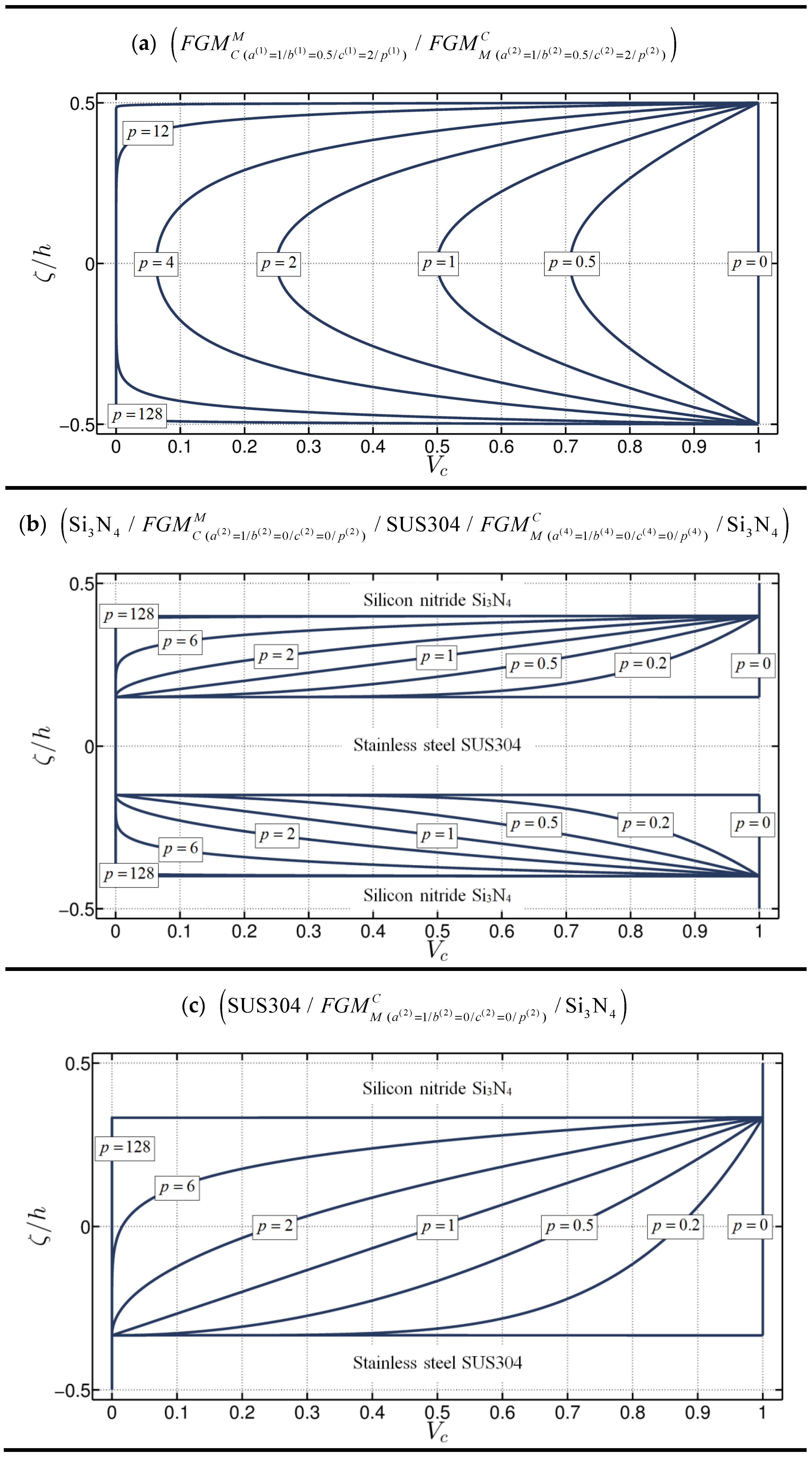
2. Functionally Graded Materials

It is well-known that FGMs allows to define a continuous gradual variation of the mechanical properties of two isotropic constituents, in general one ceramic and one metal, from the bottom to the top surfaces of the layer in which they are employed. In the present paper, the rule of mixture is used to evaluate the mechanical properties of these composites. For the sake of simplicity, let us assume that the k -th layer of the structure is made of FGM and the two constituents are ceramic and metallic materials, respectively. Each mechanical quantity related to the first constituent is denoted by the subscript “ C ”, whereas the subscript “ M ” is used to specify the properties of the metal. Since the two constituents are assumed isotropic and linear elastic, they are fully characterized through the Young’s modulus ( E C , E M ), Poisson’s ratio ( ν C , ν M ), and the density ( ρ C , ρ M ). By hypothesis, these composites are isotropic and non-homogenous along the thickness direction, which is denoted by ζ . Thus, the rule of mixture provides the following relations
E ( k ) ( ζ ) = E C V C ( k ) ( ζ ) + E M V M ( k ) ( ζ )
ν ( k ) ( ζ ) = ν C V C ( k ) ( ζ ) + ν M V M ( k ) ( ζ )
ρ ( k ) ( ζ ) = ρ C V C ( k ) ( ζ ) + ρ M V M ( k ) ( ζ )
where E ( k ) ( ζ ) , ν ( k ) ( ζ ) , and ρ ( k ) ( ζ ) stand for the overall mechanical properties of the k -th FGM layer. On the other hand, V C ( k ) ( ζ ) and V M ( k ) ( ζ ) represent the volume fraction distributions of the ceramic and the metal, respectively. These two quantities are related as follows
V C ( k ) ( ζ ) + V M ( k ) ( ζ ) = 1
Thus, Equations (1)–(3) could be rewritten also as a function only of the volume fraction of one constituent. Several expressions are available in the literature to define the continuous and gradual variation of the mechanical properties along the thickness of the FGM layer [67]. In the current paper, a four-parameter power law is introduced for this purpose. Let us assume that the volume fraction is strictly related to the materials located to the external surfaces of the k -th FGM layer. With reference to Figure 1, in which a generic stacking sequence made of FGM and isotropic layers is depicted, the k -th ply is identified by the thickness coordinates ζ k and ζ k + 1 , which denote respectively the coordinates of its bottom and top surfaces in each point of the reference domain.
On the other hand, h k represents the thickness of the k -th layer in a generic point of the domain. If the constituent at the top surface is the ceramic material, the volume fraction V C ( k ) ( ζ ) is defined as follows
V C ( k ) ( ζ ) = ( 1 a ( k ) ( ζ k + 1 ζ h k ) + b ( k ) ( ζ k + 1 ζ h k ) c ( k ) ) p ( k )
where a ( k ) , b ( k ) , c ( k ) and p ( k ) are the four parameters that characterize the distribution at issue. As specified in the paper by Tornabene [60], their value must be chosen accurately so that Equation (4) is satisfied for any value of p ( k ) . On the other hand, if the constituent at the top surface is the metallic material the volume fraction V C ( k ) ( ζ ) assumes the following aspect
V C ( k ) ( ζ ) = ( 1 a ( k ) ( ζ ζ k h k ) + b ( k ) ( ζ ζ k h k ) c ( k ) ) p ( k )
It should be noted that homogeneous and isotropic material can be obtained as a particular case of the FGM, by setting properly the value of the exponent p ( k ) . In other words, by setting p ( k ) = 0 or p ( k ) = it is possible to model an isotropic layer. In addition, it should be specified that sandwich structures can be obtained by choosing properly the volume fraction distributions of the constituents in the various plies. As a consequence, the composites are not characterized by those discontinuities at the layer interfaces that typically identify conventional laminates. At this point, a peculiar notation must be introduced to specify univocally the volume fraction distribution used to define the gradual variation of the mechanical properties. In the following, the acronyms shown below are employed for this purpose. In particular, if the Equation (5) is employed, the k -th FGM layer is denoted by
F G M M ( a ( k ) / b ( k ) / c ( k ) / p ( k ) ) C
On the other hand, the notation
F G M C ( a ( k ) / b ( k ) / c ( k ) / p ( k ) ) M
is used to specify the use of Equation (6). Finally, it is important to underline that E ( k ) ( ζ ) , ν ( k ) ( ζ ) , and ρ ( k ) ( ζ ) are all affected by the gradation laws specified in Equation (5) or (6).

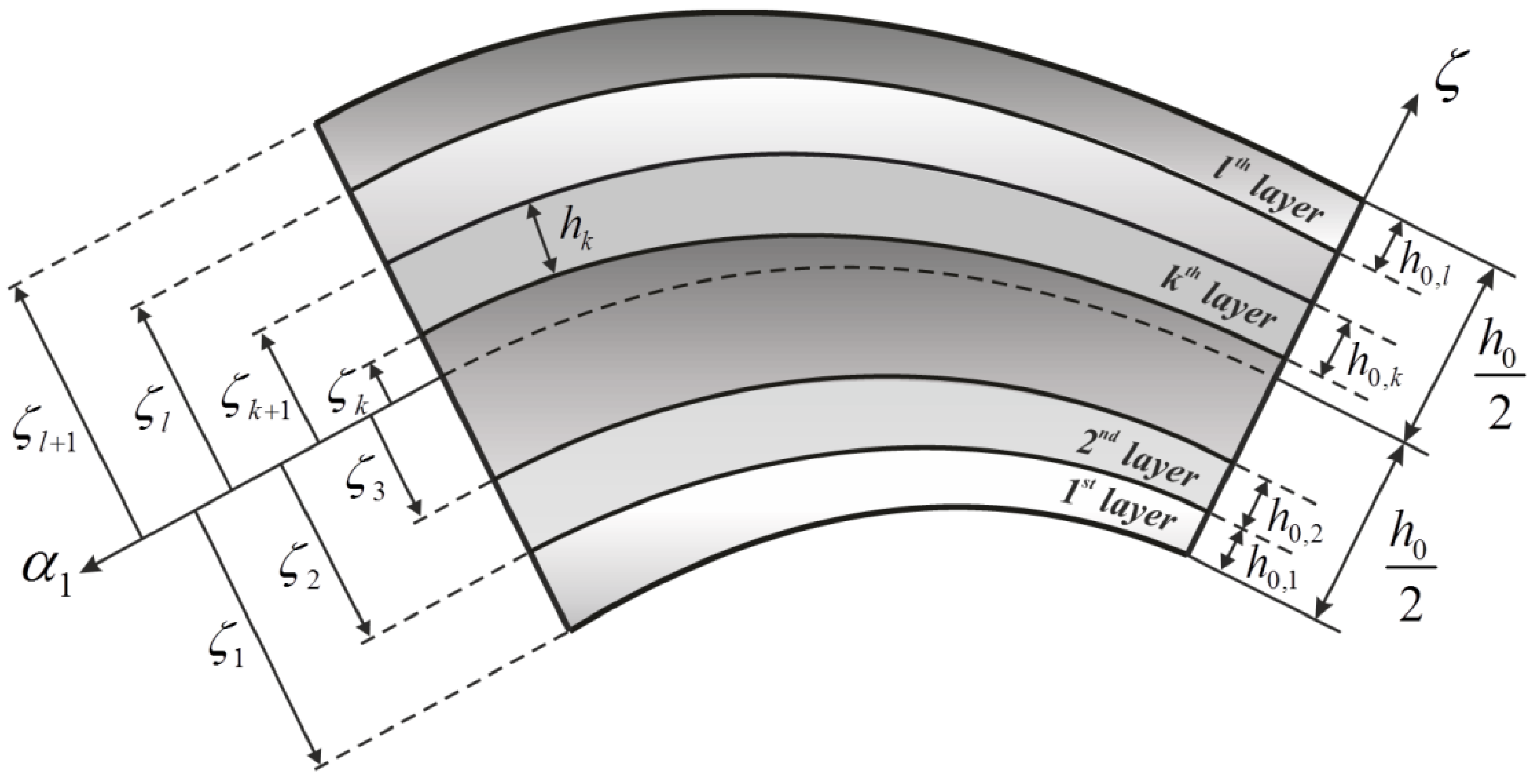
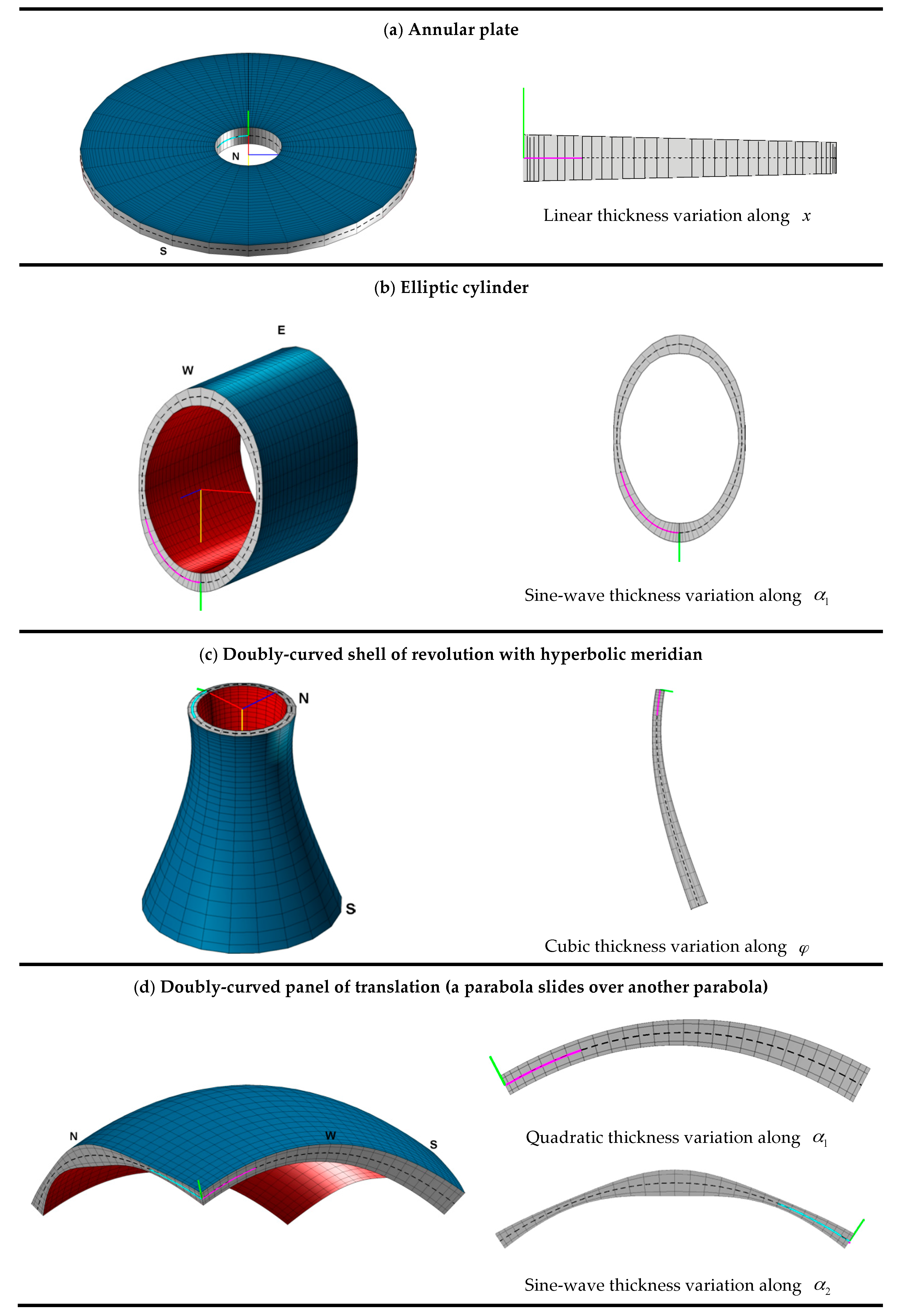
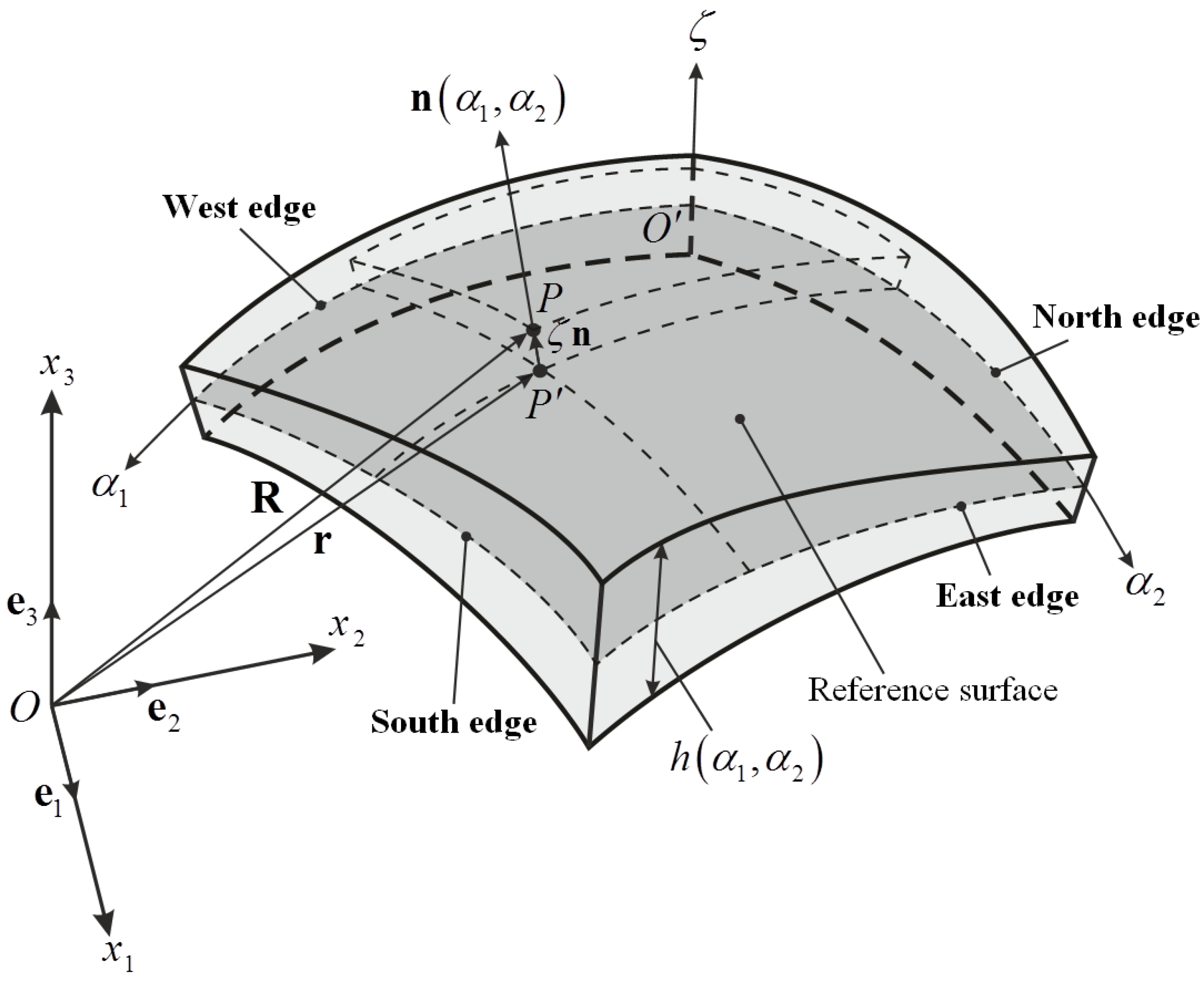
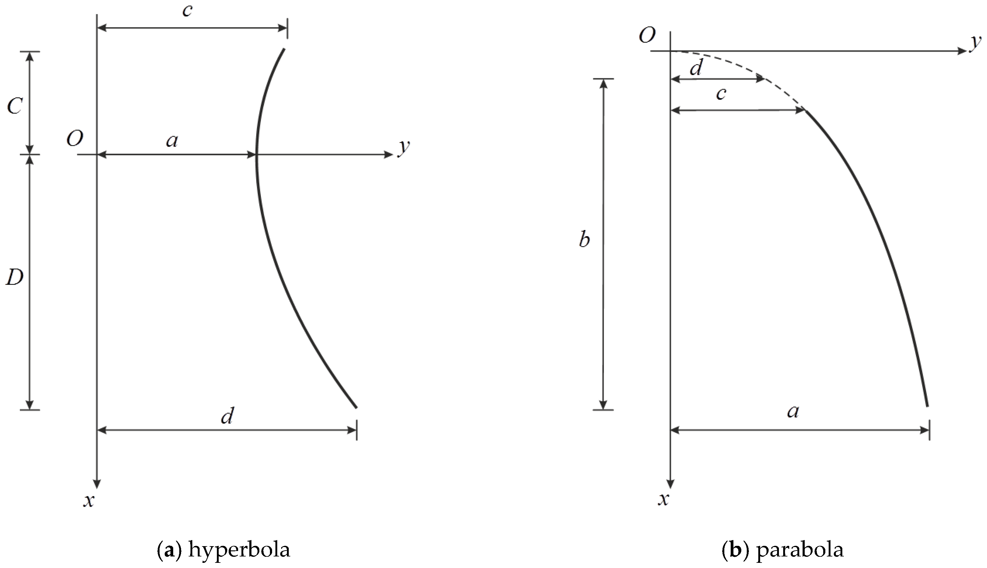
3. Definition of the Geometry

Let us consider a generic doubly-curved shell element with variable thickness as the one schematically depicted in Figure 2. It is completely identified by means of the position vector R ( α 1 , α 2 , ζ ) defined as follows
R ( α 1 , α 2 , ζ ) = r ( α 1 , α 2 ) + h ( α 1 , α 2 ) 2 z n ( α 1 , α 2 )
where z = 2 ζ / h ( α 1 , α 2 ) , for z [ 1 , 1 ] , is a non-dimensional parameter which represents the distance between the generic point P within the three-dimensional shell body and its projection P , located on the middle surface. It should be noted that O α 1 α 2 ζ denotes the local reference coordinate system of the shell element. In particular, α 1 , α 2 are the principal curvilinear coordinates of the shell middle surface, whereas ζ specify the coordinate along the normal directions, which is identified by the outward unit normal vector n ( α 1 , α 2 ) . The following boundary values must be specified to define the three-dimensional domain of the shell.
α 1 0 α 1 α 1 1
α 2 0 α 2 α 2 1
h ( α 1 , α 2 ) 2 ζ h ( α 1 , α 2 ) 2
From the definition shown in Equation (9), it is clear that the thickness of the shell h ( α 1 , α 2 ) is arbitrary and can vary point by point.
It should be recalled that its overall value is given by the sum of the thickness of each ply if the structure is made of several layers (Figure 1). Thus, one gets
h ( α 1 , α 2 ) = k = 1 l h k ( α 1 , α 2 )
where l stands for the number of layers. In the present paper, the thickness variation assumes the following aspect
h ( α 1 , α 2 ) = h 0 ( 1 + f ( α 1 ) + g ( α 2 ) )
in which h 0 is the thickness reference value, whereas f ( α 1 ) , g ( α 2 ) are arbitrary functions that describe the thickness profile along the principal curvilinear coordinates α 1 , α 2 . It should be pointed out that there is no restriction on the choice of these functions, as illustrated in details in the work by Tornabene et al. [104]. Nevertheless, they must represent a smooth variation and their effect has to involve each layer. Thus, the parameters h 0 , k , for k = 1 , 2 , ... , l , are introduced to specify the thickness reference value of each lamina. For completeness purposes, the reader can refer to the work by Tornabene et al. [104] for a general treatise on the variable thickness. In connection with Equation (9), r ( α 1 , α 2 ) is the vector that allows to identify each point of the shell reference surface, which corresponds to the middle surface of the structure. In general, its expression can be written as follows
r ( α 1 , α 2 ) = f 1 ( α 1 , α 2 ) e 1 + f 2 ( α 1 , α 2 ) e 2 + f 3 ( α 1 , α 2 ) e 3
in which f i ( α 1 , α 2 ) , for i = 1 , 2 , 3 , are generic functions that depend on the shell middle surface, whereas e i , for i = 1 , 2 , 3 , are the unit vectors which denote the main axes of the global reference system O x 1 x 2 x 3 shown in Figure 2. Equation (15) is fundamental to evaluate each geometric quantity related to the shell under consideration. For this purpose, its derivatives with respect to the principal curvilinear coordinates must be also computed. As far as the first-order derivatives are concerned, one gets
r , 1 = r α 1
r , 2 = r α 2
whereas the second-order derivatives assume the following aspect
r , 11 = 2 r α 1 2
r , 22 = 2 r α 2 2
At this point, an analytic expression can be found for the unit normal vector n ( α 1 , α 2 )
n = r , 1 r , 2 | r , 1 r , 2 |
where “ ” denotes the vector product. Analogously, the definition of the Lamè parameters A 1 ( α 1 , α 2 ) , A 2 ( α 1 , α 2 ) is also provided
A 1 = r , 1 r , 1
A 2 = r , 2 r , 2
where “ ” denotes the scalar product. Finally, the middle surface of a doubly-curved shell is characterized by two principal radii of curvature R 1 ( α 1 , α 2 ) , R 2 ( α 1 , α 2 ) that vary point by point. The following expressions can be used to define them
R 1 = r , 1 r , 1 r , 11 n
R 2 = r , 2 r , 2 r , 22 n
Equations (23) and (24) are valid since α 1 , α 2 are principal and orthogonal by hypothesis. Once definition of R 1 ( α 1 , α 2 ) , R 2 ( α 1 , α 2 ) is specified, the following quantities can be also computed
H 1 = 1 + ζ R 1
H 2 = 1 + ζ R 2
It should be specified that the parameters H 1 ( α 1 , α 2 , ζ ) , H 2 ( α 1 , α 2 , ζ ) are required to take into account the three-dimensional size of a generic shell structure. Differential geometry is the mathematical tool that allows to compute all the geometric quantities defined in the present section.

4. Higher-Order Equivalent Single Layer Approach

A unified formulation is employed in the present paper to define several HSDTs in a compact manner. In particular, an Equivalent Single Layer (ESL) approach is taken into account. The three-dimensional displacements U 1 ( α 1 , α 2 , ζ , t ) , U 2 ( α 1 , α 2 , ζ , t ) , U 3 ( α 1 , α 2 , ζ , t ) for a generic composite shell made of several layers can be written as a function of a generic order of kinematic expansion τ .
U 1 = τ = 0 N + 1 F τ ( ζ ) u 1 ( τ ) ( α 1 , α 2 , t ) U 2 = τ = 0 N + 1 F τ ( ζ ) u 2 ( τ ) ( α 1 , α 2 , t ) U 3 = τ = 0 N + 1 F τ ( ζ ) u 3 ( τ ) ( α 1 , α 2 , t )
Where the generalized displacements u 1 ( τ ) ( α 1 , α 2 , t ) , u 2 ( τ ) = u 2 ( τ ) ( α 1 , α 2 , t ) , u 3 ( τ ) = u 3 ( τ ) ( α 1 , α 2 , t ) represent the degrees of freedom of the problem and are defined on the shell middle surface. They can be conveniently collected in the algebraic vector u ( τ ) ( α 1 , α 2 , t ) for each order τ of kinematic expansion.
u ( τ ) = [ u 1 ( τ ) u 2 ( τ ) u 3 ( τ ) ] T
On the other hand, F τ ( ζ ) denotes the shear function (or thickness functions) linked to the τ -th order of kinematic expansion and can assumes different meanings. In the current work, the power function ζ τ , for τ = 0 , 1 , 2 , ... , N , is chosen for this purpose. The ( N + 1 ) -st order of kinematic expansion denotes the Murakami’s function that is employed to model the zig–zag effect [94,95,96]. For the laminated shell element shown in Figure 1, the Murakami’s function is defined as follows:
Z = ( 1 ) k ( 2 ζ k + 1 ζ k ζ ζ k + 1 + ζ k ζ k + 1 ζ k )
in which the index k is introduced to specify the k -th ply. Thus, the ( N + 1 ) -st shear function is assumed equal to Equation (29) if the zig-zag effect is included in the structural theory (in other words, one gets F N + 1 = Z ). It should be noted that each HSDT is identified by the maximum order of kinematic expansion N . If the power function ζ τ is employed to define all the thickness functions of the model, the following HSDT can be introduced.
N = 1 ED 1 N = 2 ED 2 N = 3 ED 3 N = 4 ED 4
When the zig–zag effect is contemplated, the same order theories are specified as follows:
N = 1 EDZ 1 N = 2 EDZ 2 N = 3 EDZ 3 N = 4 EDZ 4
With reference to the Equations (30) and (31), it should be noted that the letter “E” specifies an ESL model, “D” means that the fundamental equations will be written in terms of generalized displacements, and “Z” stands for the Murakami’s function. At this point it is important to underline that the displacement field of the well-known first-order shear deformation theory can be obtained from Equation (27) by choosing properly the shear functions and the degrees of freedom. In the following, this theory will be indicated by the notation FSDT (First-order Shear Deformation Theory). Analogously, the term FSDTZ is introduced to identify the FSDT embedded with the Murakami’s function.
At this point, the generalized strain components can be defined. For the sake of conciseness, they are collected in the corresponding algebraic vector ε ( τ ) ( α 1 , α 2 , t )
ε ( τ ) = [ ε 1 ( τ ) ε 2 ( τ ) γ 1 ( τ ) γ 2 ( τ ) γ 13 ( τ ) γ 23 ( τ ) ω 13 ( τ ) ω 23 ( τ ) ε 3 ( τ ) ] T
for each order τ of kinematic expansion. The generalized strain components assume the compact matrix form shown below for each order of kinematic expansion τ = 0 , 1 , 2 , ... , N , N + 1
ε ( τ ) = D Ω u ( τ )
where D Ω is the differential operator defined as
D Ω = [ 1 A 1 α 1 1 A 1 A 2 A 2 α 1 1 A 1 A 2 A 1 α 2 1 A 2 α 2 1 R 1 0 1 0 0 1 A 1 A 2 A 1 α 2 1 A 2 α 2 1 A 1 α 1 1 A 1 A 2 A 2 α 1 0 1 R 2 0 1 0 1 R 1 1 R 2 0 0 1 A 1 α 1 1 A 2 α 2 0 0 1 ] T
The internal stress resultants for each order of kinematic expansion τ = 0 , 1 , 2 , ... , N , N + 1 are collected in the algebraic vector S ( τ ) ( α 1 , α 2 , t ) which assume the following aspect.
S ( τ ) = [ N 1 ( τ ) N 2 ( τ ) N 12 ( τ ) N 21 ( τ ) T 1 ( τ ) T 2 ( τ ) P 1 ( τ ) P 2 ( τ ) S 3 ( τ ) ] T
Due to the duality between stresses and strains, the generalized stress resultants can be directly related to the corresponding generalized displacements. In compact matrix form, one gets
S ( τ ) = η = 0 N + 1 A ( τ η ) D Ω u ( η )
for τ = 0 , 1 , 2 , ... , N , N + 1 , in which A ( τ η ) is the matrix of the elastic constants. Equation (36) is of extremely importance since it gives also the definition of the stress resultants involved in those boundary conditions that affect the stresses, such as in the free edges. In general, the matrix A ( τ η ) assumes the following aspect for a shell made of l layers.
A ( τ η ) = [ A 11 ( 20 ) ( τ η ) A 12 ( 11 ) ( τ η ) A 16 ( 20 ) ( τ η ) A 16 ( 11 ) ( τ η ) 0 0 0 0 A 13 ( 10 ) ( τ η ˜ ) A 12 ( 11 ) ( τ η ) A 22 ( 02 ) ( τ η ) A 26 ( 11 ) ( τ η ) A 26 ( 02 ) ( τ η ) 0 0 0 0 A 23 ( 01 ) ( τ η ˜ ) A 16 ( 20 ) ( τ η ) A 26 ( 11 ) ( τ η ) A 66 ( 20 ) ( τ η ) A 66 ( 11 ) ( τ η ) 0 0 0 0 A 36 ( 10 ) ( τ η ˜ ) A 16 ( 11 ) ( τ η ) A 26 ( 02 ) ( τ η ) A 66 ( 11 ) ( τ η ) A 66 ( 02 ) ( τ η ) 0 0 0 0 A 36 ( 01 ) ( τ η ˜ ) 0 0 0 0 A 44 ( 20 ) ( τ η ) A 45 ( 11 ) ( τ η ) A 44 ( 10 ) ( τ η ˜ ) A 45 ( 10 ) ( τ η ˜ ) 0 0 0 0 0 A 45 ( 11 ) ( τ η ) A 55 ( 02 ) ( τ η ) A 45 ( 01 ) ( τ η ˜ ) A 55 ( 01 ) ( τ η ˜ ) 0 0 0 0 0 A 44 ( 10 ) ( τ ˜ η ) A 45 ( 01 ) ( τ ˜ η ) A 44 ( 00 ) ( τ ˜ η ˜ ) A 45 ( 00 ) ( τ ˜ η ˜ ) 0 0 0 0 0 A 45 ( 10 ) ( τ ˜ η ) A 55 ( 01 ) ( τ ˜ η ) A 45 ( 00 ) ( τ ˜ η ˜ ) A 55 ( 00 ) ( τ ˜ η ˜ ) 0 A 13 ( 10 ) ( τ ˜ η ) A 23 ( 01 ) ( τ ˜ η ) A 36 ( 10 ) ( τ ˜ η ) A 36 ( 01 ) ( τ ˜ η ) 0 0 0 0 A 33 ( 00 ) ( τ ˜ η ˜ ) ]
where
A n m    ( p q ) ( τ η ) = k = 1 l ζ k ζ k + 1 B ¯ n m ( k ) F η F τ H 1 H 2 H 1 p H 2 q d ζ A n m    ( p q ) ( τ ˜ η ) = k = 1 l ζ k ζ k + 1 B ¯ n m ( k ) F η F τ ζ H 1 H 2 H 1 p H 2 q d ζ A n m    ( p q ) ( τ η ˜ ) = k = 1 l ζ k ζ k + 1 B ¯ n m ( k ) F η ζ F τ H 1 H 2 H 1 p H 2 q d ζ A n m    ( p q ) ( τ ˜ η ˜ ) = k = 1 l ζ k ζ k + 1 B ¯ n m ( k ) F η ζ F τ ζ H 1 H 2 H 1 p H 2 q d ζ
for τ , η = 0 , 1 , 2 , ... , N , N + 1 , n , m = 1 , 2 , 3 , 4 , 5 , 6 and p , q = 0 , 1 , 2 . For the sake of conciseness, the symbols τ , η denote the shear function order, whereas τ ˜ , η ˜ stand for the corresponding derivatives with respect to ζ . On the other hand, B ¯ n m ( k ) specifies the elastic constant of the material. It assumes the following definition for n , m = 1 , 2 , 3 , 6
B ¯ n m ( k ) = E ¯ n m ( k )
whereas for n , m = 4 , 5 one gets
B ¯ n m ( k ) = κ E ¯ n m ( k )
where κ = 1 / χ is the shear correction factor. If the structural model requires this correction, the value of χ is set equal to χ = 1.2 , otherwise the unitary value is employed ( χ = 1 ). Equations (39) and (40) are general and allows to introduce also the plane stress hypothesis. In fact, E ¯ n m ( k ) denotes the elastic constant of the material of the k -th ply. If the plane stress hypothesis is required, the reduced elastic coefficients must be used ( E ¯ n m ( k ) = Q ¯ n m ( k ) ). On the other hand, the non-reduced coefficients are employed ( E ¯ n m ( k ) = C ¯ n m ( k ) ). These aspects will be specified properly by adding specific subscripts and superscripts to the notation used to denote the structural model. For instance, the Reissner-Mindlin theory needs both the shear correction factor and the plane stress-reduced elastic coefficients. As a consequence, it will be indicated as FSDT R S χ = 1.2 , where R S stands for “reduced stiffness”. Finally, it should be specified that the quantities E ¯ n m ( k ) depend on the third coordinate ζ if the layer is made of FGM. In other words, one gets E ¯ n m ( k ) ( ζ ) .
A set of three motion equations for each order of kinematic expansion τ = 0 , 1 , 2 , ... , N , N + 1 is obtained. In compact matrix form, they assume the following aspect
D Ω * S ( τ ) = η = 0 N + 1 M ( τ η ) u ¨ ( η )
The equilibrium operator D Ω * is defined as follows:
D Ω * = [ 1 A 1 α 1 + 1 A 1 A 2 A 2 α 1 1 A 1 A 2 A 1 α 2 1 R 1 1 A 1 A 2 A 2 α 1 1 A 2 α 2 + 1 A 1 A 2 A 1 α 2 1 R 2 1 A 1 A 2 A 1 α 2 1 A 1 α 1 + 1 A 1 A 2 A 2 α 1 0 1 A 2 α 2 + 1 A 1 A 2 A 1 α 2 1 A 1 A 2 A 2 α 1 0 1 R 1 0 1 A 1 α 1 + 1 A 1 A 2 A 2 α 1 0 1 R 2 1 A 2 α 2 + 1 A 1 A 2 A 1 α 2 1 0 0 0 1 0 0 0 1 ] T
On the other hand, the mass matrix M ( τ η ) is defined below:
M ( τ η ) = [ I ( τ η ) 0 0 0 I ( τ η ) 0 0 0 I ( τ η ) ]
for τ , η = 0 , 1 , 2 , ... , N , N + 1 . If ρ ( k ) stands for the mass density of the k -th layer, the inertia masses I ( τ η ) in Equation (43) are computed for each order of kinematic expansion τ , η = 0 , 1 , 2 , ... , N , N + 1 as follows
I ( τ η ) = k = 1 l ζ k ζ k + 1 ρ ( k ) F τ F η H 1 H 2 d ζ
With reference to the motion Equation (41), it should be specified that u ¨ ( η ) ( α 1 , α 2 , t ) is the algebraic vector that collects the second-order derivatives of the generalized displacements Equation (28) with respect to the time variable t . The system of governing Equation (41) can be expressed as a function of the degrees of freedom by inserting Equation (36) into (41). The fundamental equations are obtained for each order of kinematic expansion τ , η = 0 , 1 , 2 , ... , N , N + 1
η = 0 N + 1 L ( τ η ) u ( η ) = η = 0 N + 1 M ( τ η ) u ¨ ( η )
where L ( τ η ) is the fundamental operator defined as follows
L ( τ η ) = [ L 11 ( τ η ) L 12 ( τ η ) L 13 ( τ η ) L 21 ( τ η ) L 22 ( τ η ) L 23 ( τ η ) L 31 ( τ η ) L 32 ( τ η ) L 33 ( τ η ) ]
The terms collected into Equation (46) can be computed by applying the following definition
L ( τ η ) = D Ω * A ( τ η ) D Ω
for τ , η = 0 , 1 , 2 , ... , N , N + 1 . It should be pointed out that Equation (45) define a set of 3 × ( N + 2 ) motion equations. Since it represents a set of partial differential equations, the proper boundary conditions must be enforced to find the solution. At this point, Figure 2 can be taken as a reference to identify the coordinates of each edge along which the boundary conditions are applied. Let us consider fully clamped edges (specified by “C”) or free edges (denoted by “F”). The boundary conditions assume the following aspect
C u 1 ( τ ) = u 2 ( τ ) = u 3 ( τ ) = 0 F    N 1 ( τ ) = N 12 ( τ ) = T 1 ( τ ) = 0
for α 2 0 α 2 α 2 1 and α 1 = α 1 0 or α 1 = α 1 1 . This is the case of the South (S) and North (N) edges. The same boundary conditions can be written as follows:
C u 1 ( τ ) = u 2 ( τ ) = u 3 ( τ ) = 0 F    N 21 ( τ ) = N 2 ( τ ) = T 2 ( τ ) = 0
for α 1 0 α 1 α 1 1 and α 2 = α 2 0 or α 2 = α 2 1 . This is the case of the West (W) and East (E) edges. In the next sections related to the numerical applications, the boundary conditions applied along each edge will be specified following the order WSEN. Finally, it should be noted that another set of compatibility conditions must be enforced if the considered structure has a common edge, as in the case of complete shells of revolution or toroidal panels. If the closing edge involves the coordinates α 1 = α 1 0 and α 1 = α 1 1 , the following conditions must be added in terms of stress resultants
N 1 ( τ ) ( α 1 0 , α 2 , t ) = N 1 ( τ ) ( α 1 1 , α 2 , t ) N 12 ( τ ) ( α 1 0 , α 2 , t ) = N 12 ( τ ) ( α 1 1 , α 2 , t ) T 1 ( τ ) ( α 1 0 , α 2 , t ) = T 1 ( τ ) ( α 1 1 , α 2 , t )
and displacements
u 1 ( τ ) ( α 1 0 , α 2 , t ) = u 1 ( τ ) ( α 1 1 , α 2 , t ) u 2 ( τ ) ( α 1 0 , α 2 , t ) = u 2 ( τ ) ( α 1 1 , α 2 , t ) u 3 ( τ ) ( α 1 0 , α 2 , t ) = u 3 ( τ ) ( α 1 1 , α 2 , t )
On the other hand, if the closing edge is identified by α 2 = α 2 0 and α 2 = α 2 1 , the compatibility conditions in terms of stress resultants become
N 21 ( τ ) ( α 1 , α 2 0 , t ) = N 21 ( τ ) ( α 1 , α 2 1 , t ) N 2 ( τ ) ( α 1 , α 2 0 , t ) = N 2 ( τ ) ( α 1 , α 2 1 , t ) T 2 ( τ ) ( α 1 , α 2 0 , t ) = T 2 ( τ ) ( α 1 , α 2 1 , t )
whereas the kinematic conditions assume the aspect written below
u 1 ( τ ) ( α 1 , α 2 0 , t ) = u 1 ( τ ) ( α 1 , α 2 1 , t ) u 2 ( τ ) ( α 1 , α 2 0 , t ) = u 2 ( τ ) ( α 1 , α 2 1 , t ) u 3 ( τ ) ( α 1 , α 2 0 , t ) = u 3 ( τ ) ( α 1 , α 2 1 , t )
Finally, it should be specified that the presented theoretical approach is employed to analyze the mechanical behavior of thick and moderately thick shells that are defined by the following limitations
0.01 max ( h R min , h L min ) 0.2
where R min and L min stand for the minimum value of the radii of curvature and the minimum size, respectively.

5. Numerical Aspects

In this section, the numerical techniques employed in the present work are briefly illustrated. In particular, the GDQ method is used to approximate the derivatives in order to solve the strong form of the governing equations and to obtain the geometric parameters required to define the shell geometry. On the other hand, the integrals needed to evaluate the elastic constants of the stiffness matrix are computed by means of the Generalized Integral Quadrature (GIQ). For further details concerning these numerical approaches, the reader can refer to the review paper by Tornabene et al. [124].

5.1. Local Generalized Differential Quadrature Method

The Local Generalized Differential Quadrature (LGDQ) method is a numerical tool that allows to approximate the derivatives of a generic function without considering all the points of the reference domain. In other words, local interpolating basis functions are taken into account instead of their corresponding global ones, if compared to the well-known GDQ method. The main features of the LGDQ are explained in this paragraph considering a one-dimensional domain for conciseness purposes. The n -th derivative of a sufficiently smooth function f ( x ) evaluated at a generic point x i can be computed as a weighted linear sum of the function values at some selected grid points, considering only a limited part of the whole domain, which is globally made up of I N discrete points. From the mathematical point of view, one gets
d n f ( x ) d x n | x = x i j = N 1 N 2 ς i j ( n ) f ( x j )
for i   =   1 ,   2 , ... ,   I N , where the symbol ς i j ( n ) denotes the weighting coefficients for derivative in hand. It is clear that the evaluation of these weighting coefficients and the choice of a proper grid distribution represent the key points of the present technique. The limit values of the sum N 1 , N 2 depend on the position of the point x i where the derivative is computed. The following relations must be introduced to define their value
N 1 = max ( i I P N , 1 ) N 2 = min ( i + I P N , I N )
for i   =   1 ,   2 , ... ,   I N . The symbol I P N stands for the number of grid points that must be taken into account on the left and on the right of the point x i itself. It should be noted that the value of I P N has to be set a priori. Due to the definitions shown in Equation (56), the values of N 1 , N 2 is variable and assumes different meanings according to the position of the point x i within the domain. Figure 3 is introduced now to explain more clearly the significance of Equation (56). Let us assume that x i is placed in the center of the domain so that on both its left and its right the number of points is greater than I P N . As it can be noted from Figure 3a, the derivative shown in Equation (55) is computed considering ( 2 I P N + 1 ) points, since N 1 = i I P N and N 2 = i + I P N . Let us consider the circumstance in which x i is located next to the limits of the domain (or corresponds also to the boundary points). In these case, the value of I P N can be greater than the number of points that actually appear on the left (Figure 3b) or on the right (Figure 3c) of x i . With reference to the case depicted in Figure 3b, one gets N 1 = 1 and N 2 = i + I P N , whereas N 1 = i I P N and N 2 = I N is set for the situation shown in Figure 3c. It should be clear that the variability of N 1 , N 2 is given not to overcome the domain boundaries. Finally, the well-known GDQ method in its global form can be obtained by setting N 1 = 1 and N 2 = I N for each value of I P N .
As far as the evaluation of the weighting coefficients ς i j ( n ) is concerned, the formulas shown in the works [104,123] can be used. For the first-order derivatives, one gets
ς i j ( 1 ) = k = N 1 , k i , j N 2 ( x i x k ) k = N 1 , k i , j N 2 ( x j x k )           for     i j ,     j [ N 1 , N 2 ]
ς i j ( 1 ) = k = N 1 , k i N 2 ς i k ( 1 )           for     i = j ,     j [ N 1 , N 2 ]
ς i j ( 1 ) = 0           otherwise
On the other hand, the following recursive relations must be employed for the n -th order derivatives
ς i j ( n ) = n ( ς i j ( 1 ) ς i i ( n 1 ) ς i j ( n 1 ) x i x j )           for     i j ,     j [ N 1 , N 2 ]
ς i j ( n ) = k = N 1 , k i N 2 ς i k ( n )           for     i = j ,     j [ N 1 , N 2 ]
ς i j ( n ) = 0           otherwise
The formulation just presented can be easily extended to the case of two-dimensional domain following the same considerations shown in the works [108,109]. It should be noted that in this case a discrete grid distribution must be applied along both the principal coordinate directions. Let us assume that the domain is bounded by the limitations shown in Equations (10)–(12). The discrete points within the shell reference domain can be placed as follows
α 1 i = α 1 1 α 1 0 r I N r 1 ( r i r 1 ) + α 1 0
α 2 j = α 2 1 α 2 0 r I M r 1 ( r j r 1 ) + α 2 0
for i = 1 , 2 , ... , I N and j = 1 , 2 , ... , I M , where I N , I M denote the total number of points along α 1 , α 2 , respectively. Due to the general features of the present approach, several grid distributions can be considered to define the value of r i , r j . Due to the accuracy and convergence characteristics shown in the work [104], the points are placed within the domain by evaluating the roots of the Chebyshev polynomials of the second kind. In other words, r i , r j assume the following aspect
r i = cos ( I N i + 1 I N + 1 π )
r j = cos ( I M j + 1 I M + 1 π )
for i = 1 , 2 , ... , I N , j = 1 , 2 , ... , I M , and r [ 1 , 1 ] . It should be noted that a local interval of points must be defined also along the second principal direction of the two-dimensional domain. For this purpose, the parameter I P M is introduced with the same meaning of I P N . For the sake of simplicity, in the present work the value of I P M corresponds to I P N . In general, the use of the LGDQ should be more advisable to deal with those physical problems in which the properties of the domain change point by point. With this aim, a substantial number of discrete points could be required to define accurately these features, as in the case of shells with variable thickness presented in this work. As a consequence, the cost could be high from the computational point of view if a global approach is employed. Nevertheless, the LGDQ represents an efficient tool to reduce the computational effort since the matrix that collects the coefficients is banded, as explained in the literature [102,104].

5.2. Generalized Integral Quadrature Method

The GIQ method is a numerical tool that allows to evaluate integrals. Let us consider a smooth function f ( x ) defined in a closed domain [ a , b ] . In addition, let us assume that I T points are placed to discretize the domain itself, so that one gets a = x 1 , x 2 , , x I T 1 , x I T = b . As a consequence, I T 1 subdomains are defined. The continuous function f ( x ) can be approximated by the Lagrange polynomials of order I T 1 , since I T points are employed to discretize the domain. The integral of the approximated function in the closed interval [ x i , x j ] is defined as follows
x i x j f ( x ) d x = k = 1 I T w k i j f ( x k )
In other words, the numerical integral of f ( x ) is a weighted linear sum of the values that the function f ( x ) assumes in each point of the reference domain. It should be noted that this procedure involves the values that the function assumes in the points placed outside the integration domain. As in the GDQ method, w k i j are the weighting coefficients required for the integration, which can be computed as shown below. Let us assume that the function f ( x ) is approximated by a polynomial expansion as
f ( x ) = a 1 + a 2 x + + a I T x I T 1
in which a i , for i = 1 , 2 , ... , I T , denote the arbitrary constants of the polynomial. An auxiliary function F ( x ) must be introduced so that
f ( x ) = d F ( x ) d x
Due to Equation (68), the function F ( x ) can be defined as
F ( x ) = c x f ( λ ) d λ + u ( c ) = I f ( x , c ) + u ( c )
in which I f ( x , c ) is the integrand function that assumes the following aspect
I f ( x , c ) = x ( a 1 + a 2 2 x + + a I T I T x I T 1 ) c ( a 1 + a 2 2 c + + a I T I T c I T 1 )
On the other hand, c denotes an arbitrary constant. Due to the Weierstrass theorem and the properties of a linear vector space, the expression below represents an approximation of the function I f ( x , c )
I f ( x , c ) = j = 1 I T ( x c ) l j ( x ) d j
where l j ( x ) specifies the Lagrange polynomials. The first derivative of I f ( x , c ) with respect to x can be easily evaluated at the point x i
d I f ( x , c ) d x | x i = I f ( 1 ) ( x , c ) | x i = j = 1 I T d j ( l j ( x i ) + ( x i c ) l j ( 1 ) ( x i ) )
where l j ( 1 ) ( x i ) stands for the first-order derivative with respect to x of the Lagrange polynomials computed at x i . It should be noted that l j ( 1 ) ( x i ) stands for the first-order derivative with respect to x of the Lagrange polynomials computed at x i and coincides with the weighting coefficients of the first order derivative ς i j ( 1 ) given by the GDQ method [124]. By applying the differential quadrature law, Equation (73) becomes
d I f ( x , c ) d x | x i = I f ( 1 ) ( x , c ) | x i = j = 1 I T ς ¯ i j ( 1 ) I f ( x j , c ) = j = 1 I T ς ¯ i j ( 1 ) k = 1 I T d k ( x j c ) l k ( x j )
in which the terms l k ( x j ) = δ k j represent the Kronecker delta. The following results is achieved by comparing Equations (73) and (74)
d I f ( x , c ) d x | x i = I f ( 1 ) ( x , c ) | x i = j = 1 I T ς ¯ i j ( 1 ) ( x j c ) d j
where the weighting coefficients assume the form
ς ¯ i j ( 1 ) = x i c x j c ς i j ( 1 )
for i j , and
ς ¯ i j ( 1 ) = ς i i ( 1 ) + 1 x i c
for i = j . The arbitrary constant c must be set equal to c = x I T + 10 10 due to accuracy and stability reasons [124]. At this point, Equation (74) can be conveniently written in matrix form
I f ( 1 ) = ς ¯ ( 1 ) I f
in which ς ( 1 ) is the matrix that collects the weighting coefficients, and the following vectors are introduced
I f ( 1 ) = f = [ I f ( 1 ) ( x 1 , c ) , I f ( 1 ) ( x 2 , c ) , , I f ( 1 ) ( x I T 1 , c ) , I f ( 1 ) ( x I T , c ) ]
I f = F = [ I f ( x 1 , c ) , I f ( x 2 , c ) , , I f ( x I T 1 , c ) , I f ( x I T , c ) ]
Recalling Equation (70), vector I f can be rewritten as
I f = F = [ c x 1 f ( x ) d x , c x 2 f ( x ) d x , , c x I T 1 f ( x ) d x , c x I T f ( x ) d x ]
Thus, the integrals shown in Equation (81) can be evaluated as follows
I f = W I f ( 1 )
where W = ( ς ¯ ( 1 ) ) 1 is the matrix of the weighting coefficients for the integrals that can be computed by inverting the corresponding matrix of the weighting coefficients for the first-order derivatives. One gets
c x i f ( x ) d x = k = 1 I T w i k f ( x k )
for i = 1 , 2 , ... , I T . Finally, the integral in Equation (67) is obtained
c x j f ( x ) d x + c x i f ( x ) d x = c x j f ( x ) d x x i c f ( x ) d x = x i x j f ( x ) d x = k = 1 I T ( w j k w i k ) f ( x k )
where the weighting coefficients for the GIQ method are given by
w k i j = w j k w i k
It should be clear that they can be evaluated directly from the expressions of the weighting coefficients used to approximate the first order derivatives [124]. A proper grid distribution must be introduced to discretize the reference domain. Since in the present work the integrals must be evaluated along the shell thickness to compute the elastic coefficients of the stiffness matrix, the points along the coordinate ζ can be located as
ζ m = ( 1 cos ( i 1 I T 1 π ) ) h ( α 1 , α 2 ) 2 h ( α 1 , α 2 ) 2 ,
for m = 1 , 2 , ... , I T . Equation (86) represents the well-known Chebyshev–Gauss–Lobatto grid distribution. It is important to notice that each node defined by Equation (86) depends on the principal coordinates α 1 , α 2 since the thickness of the considered structures is variable. The value of I T is fixed equal to 51 for each numerical analysis presented in the following sections.

6. Free Vibration Analysis

The governing system of equations can be written in the following form
η = 0 N + 1 L ( τ η ) U ( η ) + ω 2 η = 0 N + 1 M ( τ η ) U ( η ) = 0
for τ = 0 , 1 , 2 , ... , N , N + 1 , if the solution is conveniently assumed equal to
u ( τ ) ( α 1 , α 2 , t ) = U ( τ ) ( α 1 , α 2 ) e i ω t
where U ( τ ) is the vector of the mode shapes defined as follows
U ( τ ) = [ U 1 ( τ ) ( α 1 , α 2 ) U 2 ( τ ) ( α 1 , α 2 ) U 3 ( τ ) ( α 1 , α 2 ) ] T
for each order of kinematic expansion τ . It should be noted that ω denotes the corresponding circular frequencies, from which it is possible to evaluate the natural frequencies as f = ω / 2 π .
At this point, Equation (87) can be solved by means of the LGDQ method. In other words, the derivatives that appear in the governing equation can be approximated through Equation (55) and written in their discrete form. Thus, the governing system of equations assume the following aspect
K δ = ω 2 M δ
in which K and M represent the stiffness and the mass matrices, respectively. On the other hand, δ is the vector that collects the vibration spatial amplitude values. It is well-known that Equation (90) represents a generalized linear eigenvalue problem. The eigenvalue ω k are evidently the circular frequencies of the considered structure. Once their value is computed, the corresponding eigenvectors δ k that represent the mode shapes can be evaluated, too. It should be specified that the maximum number of eigenvalues, as well as eigenvectors, depends on the number of points I N , I M chosen to discretize the reference domain along the two principal directions α 1 , α 2 , respectively. It is point out that the size of system of discrete Equation (90) is equal to 3 × ( N + 2 ) × ( I N × I M ) × ( I N × I M ) , where N denotes the maximum order of kinematic expansion. It should be noted that the size of the problem can be reduced by applying the well-known kinematic condensation of non-domain degrees of freedom in order to separate the quantities associated with the central points of the domain from the ones related to the boundaries.

7. Numerical Results

The four structures with variable thickness made of FGMs depicted in Figure 4 are considered in the present section to evaluate their natural frequencies by the LGDQ method. As previously illustrated, the reference domain (or middle surface) is described by the corresponding position vector r ( α 1 , α 2 ) , whereas a proper expression is introduced to define the smooth thickness variation of the shells. With reference to Figure 4, it should be specified that the shell cross-sections affected by the thickness variation are represented, too. To this end, the local coordinate reference system is also depicted to understand more clearly the thickness variation (the principal axes are specified by the colors magenta, cyan and green, respectively). Different stacking sequences and volume fraction distributions are taken into account to characterize the mechanical features of the composites (Figure 5). The two isotropic constituents and their corresponding properties are listed in Table 1 for conciseness purposes.
Firstly, the proposed method is validated by the comparison with the results available in the literature. Then, several parametric investigations are performed to show the effect of the variation of the volume fraction distributions on the natural frequencies. In these circumstances, the results are compared with the ones obtained by a three-dimensional finite element model (3D-FEM) for the limit cases. In other words, the commercial code Abaqus is employed only to evaluate the natural frequencies of composite structures made of isotropic layers. For this purpose, the three-dimensional model is obtained by using 20-node hexahedrons elements (C3D20). On the other hand, all the results shown in the following tables are obtained by the LGDQ method implemented in a MATLAB code [128]. In the present solution, the degrees of freedom are equal to 3 ( N + 2 ) × ( I N × I M ) , or 3 ( N + 1 ) × ( I N × I M ) in case the Murakami’s function is neglected in the HSDT.

7.1. Comparison with the Literature

The FGM annular plate defined in the work by Efraim and Eisenberger [90] is considered in the current section to validate the proposed approach. The plate middle surface is described by the following position vector
r ( x , ϑ ) = ( R i + x ) cos ϑ e 1 ( R i + x ) sin ϑ e 2
where x , ϑ are the principal coordinate of the surface, assuming x [ 0 , L ] and ϑ [ 0 , 2 π ] . The inner radius is denoted by R i , whereas the outer one can be computed as R o u t = R i + L . A linear variation is applied along the radial direction to define the thickness profile
h ( x ) = H ( 1.2 0.4 x L )
in which H is a constant parameter. The following relations must be taken into account to describe completely the plate geometry
H / R o u t = 0.1
R i / R o u t = 0.2
For the sake of completeness, both the structure and its radial cross-section are depicted in Figure 4a. The upper surface of the plate is made of Silicon nitride and a linear variation of the mechanical properties is assumed to describe the functionally graded composite layer. On the other hand, the lower surface is completely made of Stainless steel. The first 20 natural frequencies (apart from free body motions) are shown in Table 2 in their dimensionless form
Ω = 2 π f R o u t ρ M E M
As far as the boundary conditions are concerned, the structure is taken completely free (FF). The LGDQ solutions are obtained by setting I N = I M = 41 and I P N = I P M = 14 . Three different structural models are considered: FSDT R S χ = 1.2 , ED 2 χ = 1.2 , and ED 3 . It should be noted that both the first and second order theories require the shear correction factor χ = 1.2 , whereas the hypothesis of plane stress is take into account only in the FSDT. From the results shown in Table 2, it can be noted that the numerical values are in good agreement with the reference solutions for each model.

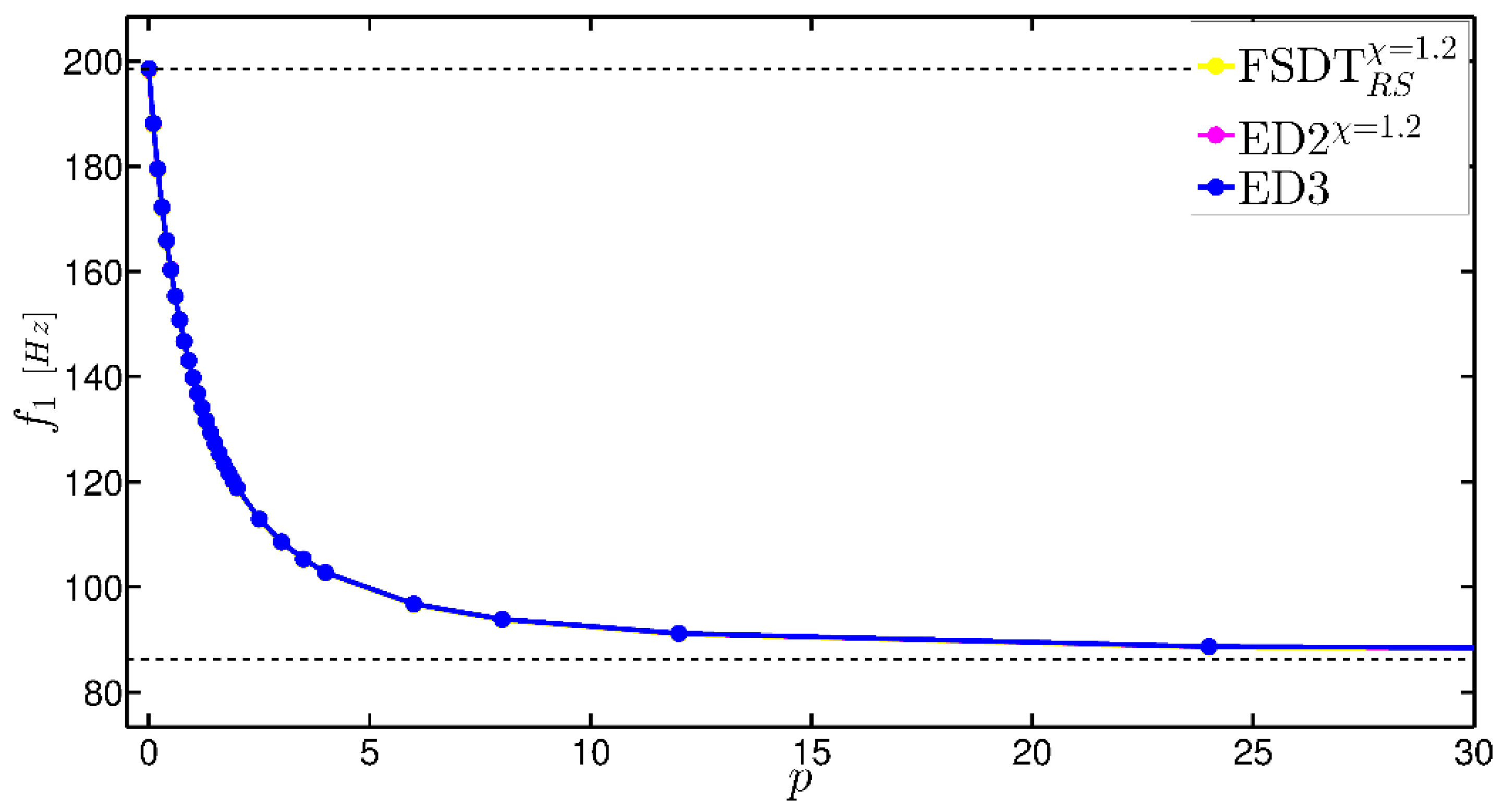
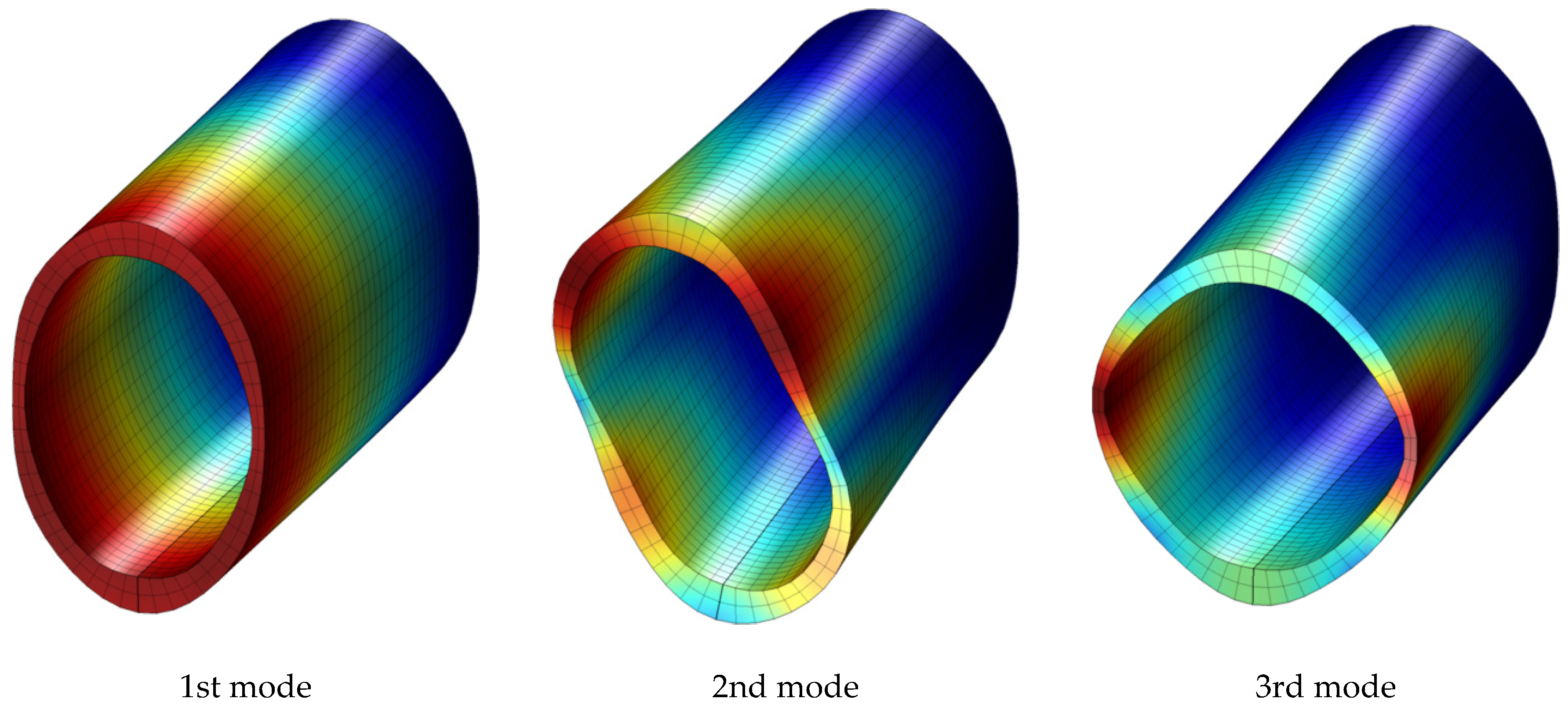
7.2. Elliptic Cylinder

The next application aims to evaluate the natural frequencies of a FC elliptic cylinder made of two FGM layers of equal thickness. The geometry under consideration is depicted in Figure 4b. The stacking sequence, as well as the volume fraction distribution of the constituents, are shown in Figure 5a for different values of the exponent p ( 1 ) = p ( 2 ) = p . The middle surface of the shell is given by the following position vector
r ( α 1 , y ) = a cos α 1 e 1 y e 2 + b sin α 1 e 3
where a = 1    m and b = 1.5    m are the semi diameters of the ellipse. The coordinates α 1 , y are bounded respectively by the limitations α 1 [ α 1 0 , α 1 1 ] and y [ 0 , L ] , with α 1 0 = π / 2 , α 1 1 = 3 π / 2 , and L = 4    m . A sine-wave variation is applied along the first coordinate α 1 to define the thickness profile. Mathematically speaking, the thickness is described by the following expression
h ( α 1 ) = h 0 ( 1 + 1 2 ( sin ( π ( 4 α 1 α 1 0 α 1 1 α 1 0 + 1 2 ) ) ) 3 )
with h 0 = 0.2    m . The first 10 natural frequencies for the considered structure are shown in Table 3 for different values of the parameter p [ 0 , ] , varying the structural model. As in the previous example, the FSDT R S χ = 1.2 , ED 2 χ = 1.2 , and ED 3 are employed. The same considerations concerning the shear correction factor and the reduced elastic stiffnesses are still valid.
It should be noted that the boundary values of p denote a structure completely made of Silicon nitride ( p = 0 ) and Stainless steel ( p = ), respectively. In this cases, the comparison with the 3D-FEM solutions is performed with excellent results for all the structural theories. It should be noted that the finite element model is made of 69680 brick elements (924690 degrees of freedom). On the other hand, the LGDQ solutions is obtained by setting I N = 51 , I M = 31 , and I P N = I P M = 16 . These values are chosen to describe accurately both the elliptical shape and the thickness variation. For completeness purposes, the variation of the first natural frequency is depicted graphically in Figure 6 as a function of the exponent p . It is evident that for lower values of p the frequencies are highly affected by variation of the volume fraction distribution of the constituents. On the other hand, for p > 4 ÷ 6 the variation in terms of natural frequencies is considerably restricted. The same behavior can be observed for each structural model. In the same plots, the black dashed lines represent the extreme cases of the isotropic homogeneous shell ( p = 0 and p = ) and the corresponding frequencies are evaluated by the finite element software. For the sake of conciseness, Figure 6 shows only the variation of the first natural frequency, but it should be specified that higher modes exhibit the same trend. It is evident that the variation of the natural frequencies is bounded by these two lines. Finally, the first three mode shapes for a FC elliptic cylinder with variable thickness are shown in Figure 7 assuming p = 1 , which corresponds to a linear distribution of the volume fraction. From these images, it can be noted that the boundary conditions are well-enforced. In this paper, the colormap used for the mode shapes stands for the intensity of the modal displacements. A zero displacement is specified by a dark blue color, whereas a red tone represents bigger movements.

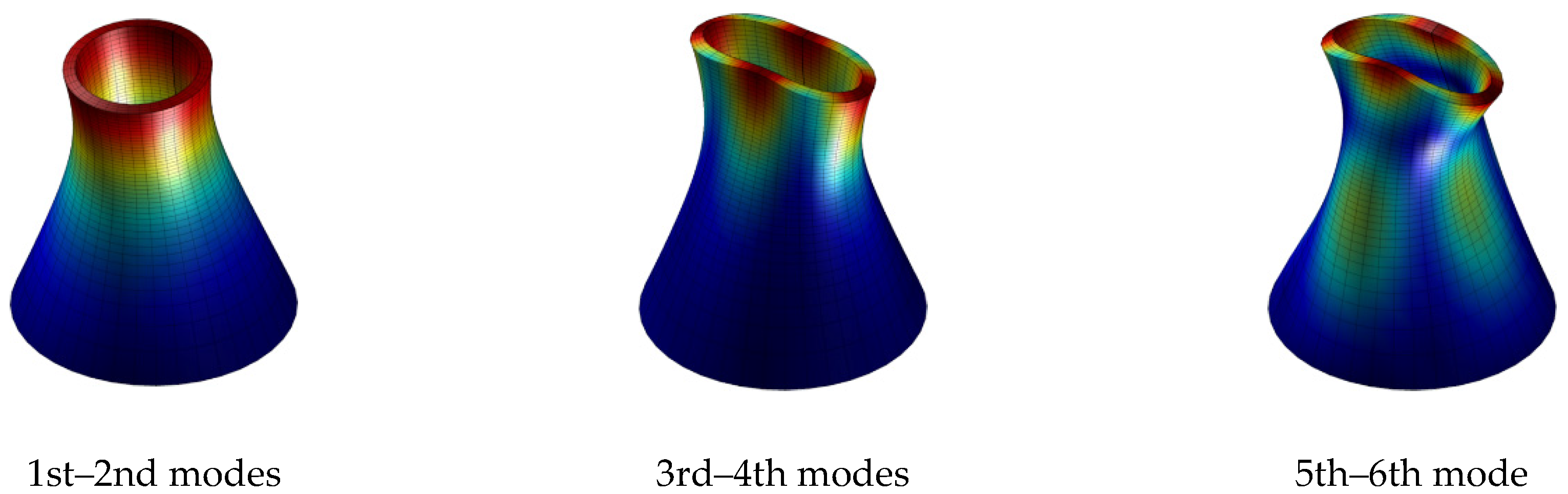
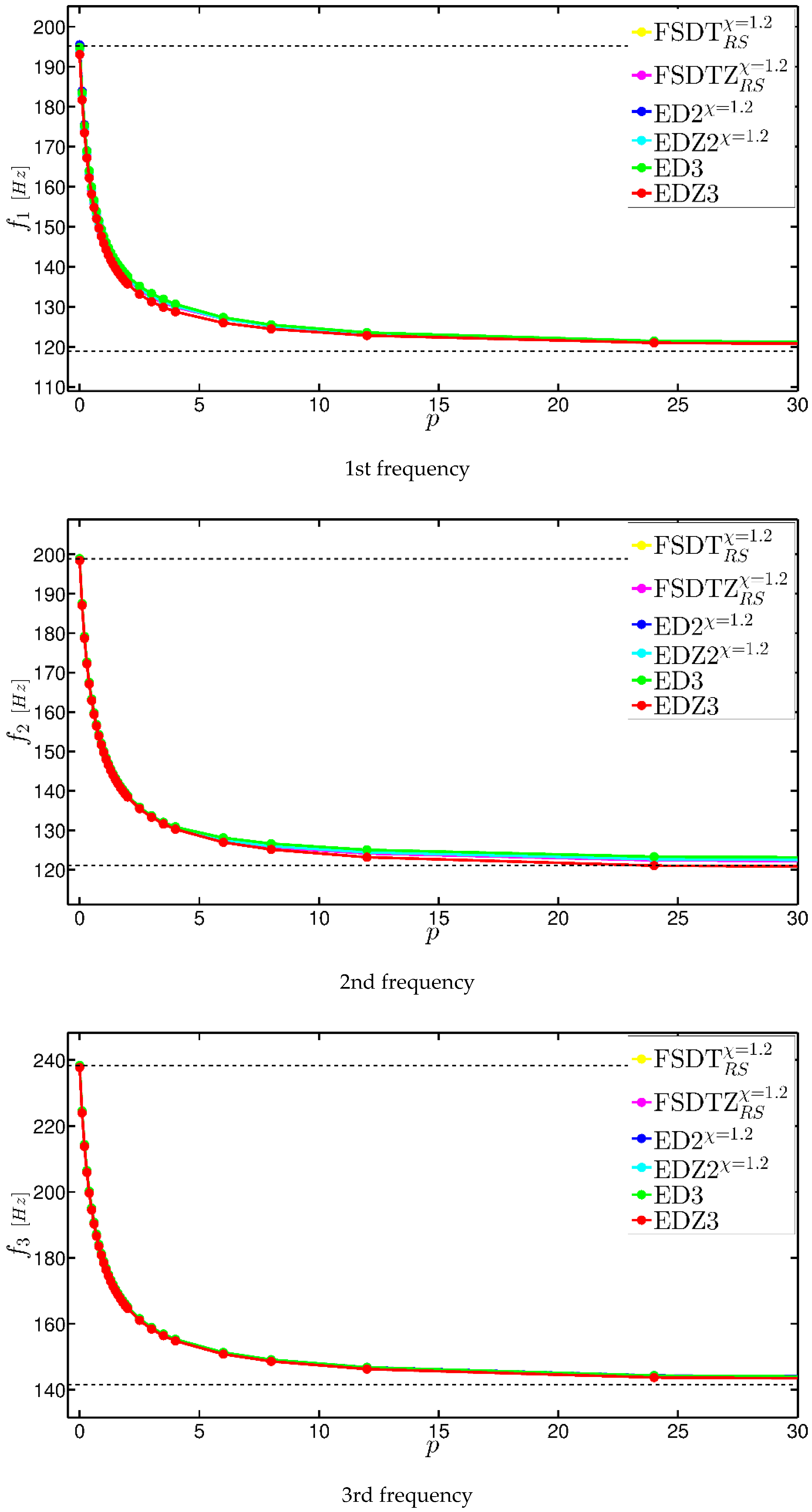
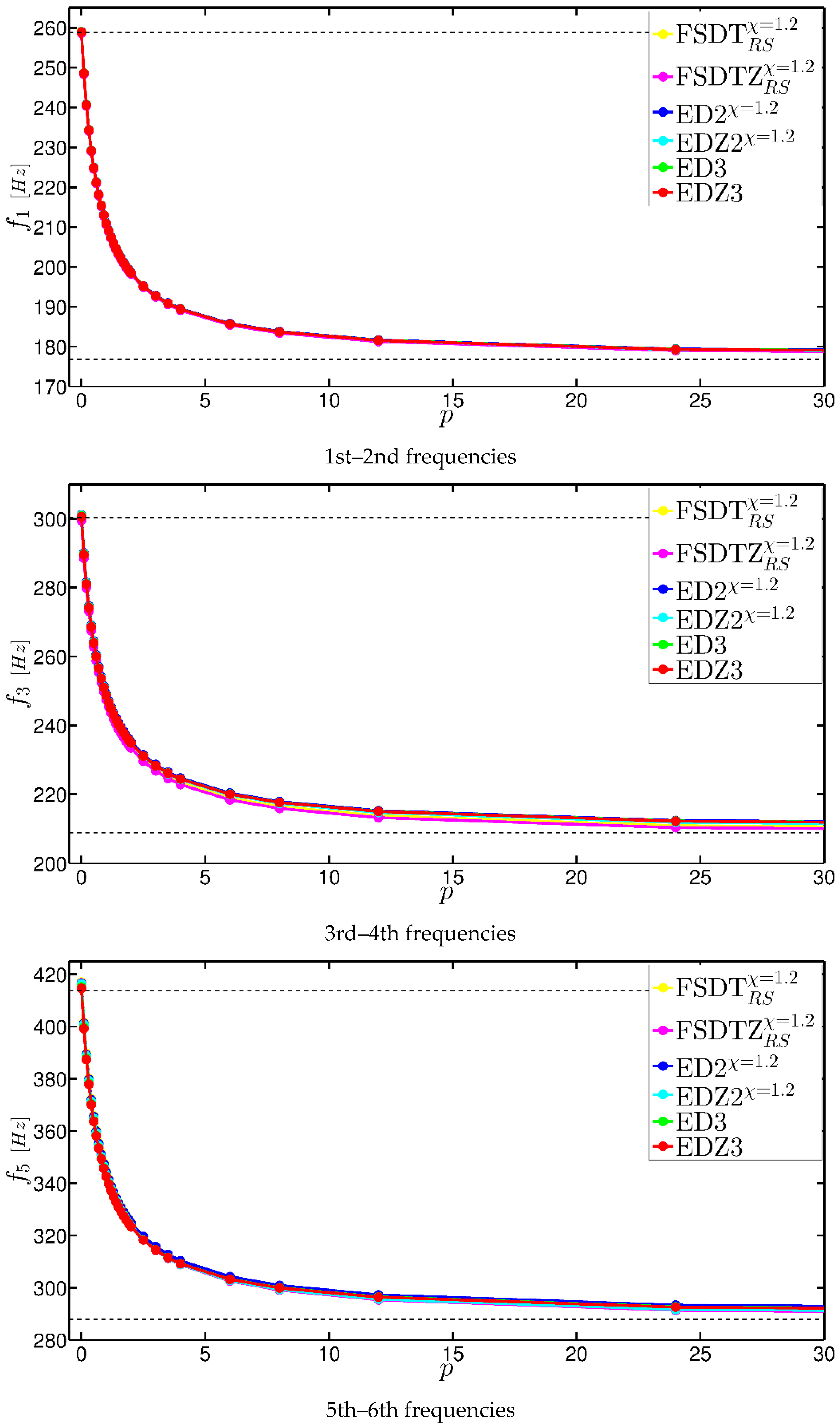
7.3. Doubly-Curved Shell of Revolution with Hyperbolic Meridian

The FC hyperbolic meridian shell, depicted in Figure 4c, is a doubly-curved shell of revolution whose reference surface is defined a branch of a hyperbola. The surface at issue is described by the following position vector
r ( φ , ϑ ) = R 0 ( φ ) cos ϑ e 1 R 0 ( φ ) sin ϑ e 2 + ( R 0 ( φ ) ) 2 a 2 k 2 1 e 3
The coordinates φ , ϑ are defined in the intervals φ [ φ 0 , φ 1 ] and ϑ [ ϑ 0 , ϑ 1 ] , where φ 0 = 1.741190 , φ 1 = 1.212026 , ϑ 0 = 0 , ϑ 1 = 2 π . On the other hand, the parallel radius R 0 ( φ ) assumes the aspect shown below
R 0 ( φ ) = a sin φ k 2 1 k 2 sin 2 φ 1
where k = 1 + a 2 / b 2 . It should be specified that a is the parallel radius of the throat section of the structure, and b = a D / d 2 a 2 is the characteristic dimension of the shell, in which a = 1    m , d = 2    m , D = 4    m . The meaning of these parameters, as well as the ones needed to sketch the following structure, can be found in Figure 8. For further details concerning the present geometry the reader can refer to the book by Tornabene et al. [2]. With reference to Figure 8a, the characteristic dimension of the hyperbola can be defined alternatively as b = a C / c 2 a 2 , where c is the parallel radius at the top section of the structure and C represents its coordinate that in the present case is equal to C = 1    m . The value of c can be computed by means of Equation (99). The reference value of thickness is h 0 = 0.2    m and it is measured along the top edge. A cubic variation is applied along the first coordinate φ and it can be defined as follows:
h ( φ ) = h 0 ( 1 + 2 ( φ φ 0 φ 1 φ 0 ) 3 )
It should be noted that the same thickness variation affects each ply, as it can be observed in the cross-section of Figure 4c. The structure is made of five layers with different thickness reference values. The two external laminae are isotropic and fully ceramic ( h 0 , 1 = h 0 , 5 = 0.02    m ), whereas the inner isotropic core is made of metal and its thickness is equal to h 0 , 3 = 0.06    m . The remaining two plies have equal thickness h 0 , 2 = h 0 , 4 = 0.05    m and are graded as it can be noted from the stacking sequence depicted in Figure 5b, where the volume fraction distributions of the two constituents are also specified for several values of the exponent p ( 2 ) = p ( 4 ) = p [ 0 , ] . In a similar way to the previous example, the boundary values of p define respectively a layer fully made of Silicon nitride ( p = 0 ) and Stainless steel ( p = ). The results of this parametric study are given in Table 4 for the FSDT R S χ = 1.2 , ED 2 χ = 1.2 , and ED 3 models.
Due to the presence of various layers with different mechanical properties, the influence of the Murakami’s function is also investigated. Thus, the aforementioned structural theories are also embedded with this function. The results related to the FSDTZ R S χ = 1.2 , EDZ 2 χ = 1.2 , and EDZ 3 models are shown in Table 5. Even in this circumstance, the shear correction factor is used for the first and second order models, whereas the plane stress hypothesis is considered only in the Reissner-Mindlin theory. It is easy to notice that the Murakami’s function does not significantly affect the results. Both in Table 4 and Table 5, the 3D-FEM solutions are also included for comparison purposes. It should be noted that the finite element model is made of 52,734 brick elements (685,824 degrees of freedom). Excellent agreement with the reference solutions is achieved in each circumstance. The LGDQ results are obtained by setting I N = I M = 31 and I P N = I P M = 16 , and the natural frequencies are written for different values of p . It should be noted that Table 4 and Table 5 show the first 18 natural frequencies. In fact, some couples of natural frequencies are equal due to the symmetry of the structure, in terms of both geometry and materials. For the sake of clarity, the variation of the first six natural frequencies as a function of the exponent p are depicted in graphical form in Figure 9 for all the considered structural models, with and without the Murakami’s function. As in the previous case, a remarkable difference in the structural response can be obtained for lower values of the parameter p . Finally, the first six mode shapes for the doubly-curved shell of revolution with hyperbolic meridian with variable thickness are shown in Figure 10 assuming a linear variation for the volume fraction distributions of the two constituents in the FGM layers ( p = 1 ).

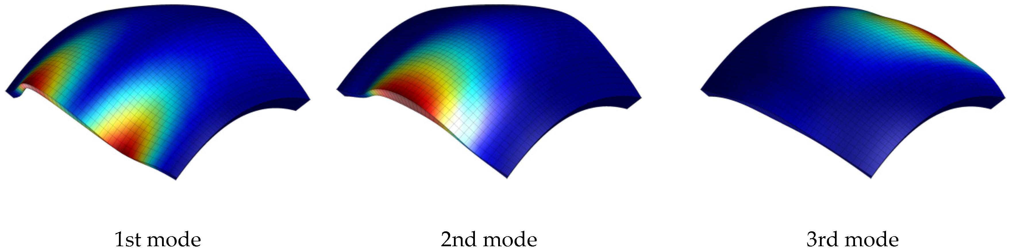
7.4. Doubly-Curved Panel of Translation

As last example, a CFCF doubly-curved panel of translation is considered (Figure 4d). Since its geometry is obtained by moving a parabola over another parabola defined by the same shape, this structure is named also as elliptic paraboloid. Its position vector can be written as follows
r ( α 1 , α 2 ) = ( k tan α 1 2 k tan 2 α 2 4 sin α 1 ) e 1 k tan α 2 2 e 2 + ( k tan 2 α 1 4 + k tan 2 α 2 4 cos α 1 ) e 3
in which the coordinates α 1 , α 2 are defined in the intervals α 1 [ α 1 0 , α 1 1 ] and α 2 [ α 2 0 , α 2 1 ] , assuming α 1 0 = α 2 0 = 0.588003 , α 1 1 = α 2 1 = 0.588003 . On the other hand, k = ( a 2 d 2 ) / b is the characteristic parameter of the two parabolas.
It is well-known that a parabolic curve is completely defined by the definition of three points with abscissas a , c , d and the relative distance b between the points of coordinates a and d . In particular, a and c represent the abscissas of the extreme points of the parabolic arch as it can be deducted from Figure 8b. The current geometry can be obtained by setting a = 3    m , b = 1    m , c = 3    m , and d = 0    m . For extra details concerning the present shape, the book by Tornabene et al. [2] can be taken into account as a reference.
As it can be noted from Figure 5c, the structure is made of three layers. In particular, the lower ply is isotropic and fully metal (Stainless steel), and the upper one is completely ceramic (Silicon nitride). These two layers have the same reference thickness h 0 , 1 = h 0 , 3 = 0.05    m . On the other hand, the central core is graded between these two limit cases and its reference thickness is equal to h 0 , 2 = 0.2    m . Thus, the overall shell thickness that can be assumed as a reference is h 0 = 0.3    m . Varying the exponent p ( 2 ) = p [ 0 , ] of the volume fraction distribution, several mechanical configurations can be obtained.
As far as the thickness profile is concerned, the thickness variation affects both the two principal coordinates α 1 , α 2 , as it can be easily observed in the cross-sections shown in Figure 4d. In particular, a quadratic variation is applied along α 1 , whereas a sine-wave variation is applied on the second direction. Mathematically speaking, the thickness of the shell at issue is defined as follows
h ( α 1 , α 2 ) = h 0 ( 1 + 3 4 ( α 1 α 1 0 α 1 1 α 1 0 ) 2 + 1 2 sin ( π ( 3 ( α 2 α 2 0 α 2 1 α 2 0 ) + 1 ) ) )
Even in this circumstance, the three structural models previously employed are taken with and without the Murakami’s function. The natural frequencies related to the FSDT R S χ = 1.2 , ED 2 χ = 1.2 , and ED 3 are shown in Table 6, whereas the ones obtained by using the FSDTZ R S χ = 1.2 , EDZ 2 χ = 1.2 , and EDZ 3 are written in Table 7, for several values of the parameter p . For the sake of completeness, the 3D-FEM solutions, which are really close to the LGDQ ones, are also included in these tables. It should be specified that the finite element model is obtained by using 51,350 brick elements (676,302 degrees of freedom).
On the other hand, the present results are obtained by setting I N = I M = 31 and I P N = I P M = 16 . From the values in Table 6 and Table 7, it is clear that the same observations illustrated for the previous case do not lose their validity. The variation of the first three natural frequencies for the doubly-curved panel of translation with variable thickness in hand is depicted in Figure 11. Finally, Figure 12 shows the first three mode shapes for p = 1 as exponent of the volume fraction distribution of the FGM layer.

8. Conclusions

The GDQ method has been applied according to a local scheme to compute natural frequencies of shell structures with variable thickness made of FGMs. The thickness profiles have been defined through a number of smooth functions (linear, power-law, sinusoidal, and their combinations), whereas a four-parameter power law function has been adopted to describe the through-the-thickness volume fraction distribution of the two constituents. As a consequence, the considered shells have been characterized by a variation of the mechanical properties both along the thickness and within the reference domain. It should be noted that the higher-order based structural models employed in this paper are two-dimensional and have allowed to evaluate accurately the natural frequencies of variable thickness structures. The same geometries have been analyzed, for verification purposes, also by means of a FEM commercial code for specific mechanical configurations. In this circumstance, a three-dimensional model made of many brick elements has been required to model the variable thickness profiles, considerably increasing the computational effort. In addition, the cost of computation has been further reduced by the use of the LGDQ method, which does not take in account all the discrete points within the domain. Consequently, the thickness variation has been described precisely by setting more grid points, without affecting the computational resources. Finally, a parametric investigation has been carried out to analyze the effect of the graded mechanical properties along the shell thickness varying the exponent of the volume fraction distributions, for several structural theories defined by different orders of kinematic expansion. The validity of the current approach has been proven for FGM structures with variable thickness through the comparison with the results available in the literature. To sum up, it has been shown that the LGDQ approach can be considered as an efficient method to solve the free vibration problem of shell structures with variable thickness with a reduced computational cost if compared to the corresponding FEM models, which required a three-dimensional description characterized by a higher number of degrees of freedom to obtain comparable results.

Acknowledgments

The research topic is one of the subjects of the Centre of Study and Research for the Identification of Materials and Structures (CIMEST)—Michele Capurso of the University of Bologna (Italy).

Author Contributions

The authors Francesco Tornabene, Nicholas Fantuzzi, Michele Bacciocchi, Erasmo Viola and Junuthula N. Reddy contributed equally to this work.

Conflicts of Interest

The authors declare no conflict of interest. The founding sponsors had no role in the design of the study; in the collection, analyses, or interpretation of data; in the writing of the manuscript, and in the decision to publish the results.

References

  1. Reddy, J.N. Mechanics of Laminated Composite Plates and Shells; CRC Press: Boca Raton, FL, USA, 2004. [Google Scholar]
  2. Tornabene, F.; Fantuzzi, N.; Bacciocchi, M.; Viola, E. Laminated Composite Doubly-Curved Shell Structures. Differential Geometry. Higher-Order Structural Theories; Esculapio: Bologna, Italy, 2016. [Google Scholar]
  3. Tornabene, F.; Fantuzzi, N.; Bacciocchi, M.; Viola, E. Laminated Composite Doubly-Curved Shell Structures. Differential and Integral Quadrature. Strong Formulation Finite Element Method; Esculapio: Bologna, Italy, 2016. [Google Scholar]
  4. Kraus, H. Thin Elastic Shells; John Wiley & Sons: New York, NY, USA, 1967. [Google Scholar]
  5. Gutierrez Rivera, M.; Reddy, J.N.; Amabili, M. A new twelve-parameter spectral/hp shell finite element for large deformation analysis of composite shells. Compos. Struct. 2016, 151, 183–196. [Google Scholar] [CrossRef]
  6. Groh, R.M.J.; Weaver, P.M. A computationally efficient 2D model for inherently equilibrated 3D stress predictions in heterogeneous laminated plates. Part I: Model formulation. Compos. Struct. 2016, 156, 171–185. [Google Scholar] [CrossRef]
  7. Groh, R.M.J.; Weaver, P.M. A computationally efficient 2D model for inherently equilibrated 3D stress predictions in heterogeneous laminated plates. Part II: Model validation. Compos. Struct. 2015, 156, 186–217. [Google Scholar] [CrossRef]
  8. Amabili, M. A new third-order shear deformation theory with non-linearities in shear for static and dynamic analysis of laminated doubly curved shells. Compos. Struct. 2015, 128, 260–273. [Google Scholar] [CrossRef]
  9. Maturi, D.A.; Ferreira, A.J.M.; Zenkour, A.M.; Mashat, D.S. Analysis of Laminated Shells by Murakami’s Zig–Zag Theory and Radial Basis Functions Collocation. J. Appl. Math. 2013, 2013, 1–14. [Google Scholar] [CrossRef]
  10. Wang, Q.; She, D.; Pang, F.; Liang, Q. Vibrations of Composite Laminated Circular Panels and Shells of Revolution with General Elastic Boundary Conditions via Fourier-Ritz Method. Curved Layer. Struct. 2016, 3, 105–136. [Google Scholar] [CrossRef]
  11. Piskunov, V.G.; Verijenko, V.E.; Adali, S.; Summers, E.B. A Higher-order Theory for the Analysis of Laminated Plates and Shells with Shear and Normal Deformation. Int. J. Eng. Sci. 1993, 31, 967–988. [Google Scholar] [CrossRef]
  12. Wu, C.P.; Hung, Y.C. Asymptotic theory of laminated circular conical shells. Int. J. Eng. Sci. 1999, 37, 977–1005. [Google Scholar] [CrossRef]
  13. Brischetto, S. An exact 3d solution for free vibrations of multilayered cross-ply composite and sandwich plates and shells. Int. J. Appl. Mech. 2014, 6, 1450076. [Google Scholar] [CrossRef]
  14. Brischetto, S.; Torre, R. Exact 3D solutions and finite element 2D models for free vibration analysis of plates and cylinders. Curved Layer. Struct. 2014, 1, 59–92. [Google Scholar] [CrossRef]
  15. Le, K.C.; Yi, J.-H. An asymptotically exact theory of smart sandwich shells. Int. J. Eng. Sci. 2016, 106, 179–198. [Google Scholar]
  16. Ye, T.; Jin, G.; Zhang, Y. Vibrations of composite laminated doubly-curved shells of revolution with elastic restraints including shear deformation, rotary inertia and initial curvature. Compos. Struct. 2015, 133, 202–225. [Google Scholar] [CrossRef]
  17. Shirakawa, K. Bending of plates based on improved theory. Mech. Res. Commun. 1985, 10, 205–211. [Google Scholar] [CrossRef]
  18. Alibeigloo, A.; Shakeri, M.; Kari, M.R. Free vibration analysis of antisymmetric laminated rectangular plates with distributed patch mass using third-order shear deformation theory. Ocean. Eng. 2008, 35, 183–190. [Google Scholar] [CrossRef]
  19. Xiang, S.; Wang, K.-M. Free vibration analysis of symmetric laminated composite plates by trigonometric shear deformation theory and inverse multiquadric RBF. Thin-Walled Struct. 2009, 47, 304–310. [Google Scholar] [CrossRef]
  20. Thai, H.-T.; Kim, S.-E. Free vibration of laminated composite plates using two variable refined plate theory. Int. J. Mech. Sci. 2010, 52, 626–633. [Google Scholar] [CrossRef]
  21. Kumar, A.; Chakrabarti, A.; Bhargava, P. Vibration of laminated composites and sandwich shells based on higher order zigzag theory. Eng. Struct. 2013, 56, 880–888. [Google Scholar] [CrossRef]
  22. Sahoo, R.; Singh, B.N. A new trigonometric zigzag theory for buckling and free vibration analysis of laminated composite and sandwich plates. Compos. Struct. 2014, 117, 316–332. [Google Scholar] [CrossRef]
  23. Vidal, P.; Polit, O.; D’Ottavio, M.; Valot, E. Assessment of the refined sinus plate finite element: Free edge effect and Meyer-Piening sandwich test. Finite Elem. Anal. Des. 2014, 92, 60–71. [Google Scholar] [CrossRef]
  24. Wang, X.; Shi, G. A refined laminated plate theory accounting for the third-order shear deformation and interlaminar transverse stress continuity. Appl. Math. Model. 2015, 39, 5659–5680. [Google Scholar] [CrossRef]
  25. Zuo, H.; Yang, Z.; Chen, X.; Xie, Y.; Miao, H. Analysis of laminated composite plates using wavelet finite element method and higher-order plate theory. Compos. Struct. 2015, 131, 248–258. [Google Scholar] [CrossRef]
  26. Malekzadeh, P.; Farid, M.; Zahedinejad, P. A three-dimensional layerwise-differential quadrature free vibration analysis of laminated cylindrical shells. Int. J. Press. Vessels Pip. 2008, 85, 450–458. [Google Scholar] [CrossRef]
  27. Malekzadeh, P.; Afsari, A.; Zahedinejad, P.; Bahadori, R. Three-dimensional layerwise-finite element free vibration analysis of thick laminated annular plates on elastic foundation. Appl. Math. Model. 2010, 34, 776–790. [Google Scholar] [CrossRef]
  28. Mantari, J.L.; Oktem, A.S.; Guedes Soares, C. A new trigonometric layerwise shear deformation theory for the finite element analysis of laminated composite and sandwich plates. Comput. Struct. 2012, 94–95, 45–53. [Google Scholar] [CrossRef]
  29. Thai, C.H.; Ferreira, A.J.M.; Carrera, E.; Nguyen-Xuan, H. Isogeometric analysis of laminated composite and sandwich plates using a layerwise deformation theory. Compos. Struct. 2013, 104, 196–214. [Google Scholar] [CrossRef]
  30. Mantari, J.L.; Guedes Soares, C. Generalized layerwise HSDT and finite element formulation for symmetric laminated and sandwich composite plates. Compos. Struct. 2013, 105, 319–331. [Google Scholar] [CrossRef]
  31. Guo, Y.; Nagy, A.P.; Gürdal, Z. A layerwise theory for laminated composites in the framework of isogeometric analysis. Compos. Struct. 2014, 107, 447–457. [Google Scholar] [CrossRef]
  32. Boscolo, M.; Banerjee, J.R. Layer-wise dynamic stiffness solution for free vibration analysis of laminated composite plates. J. Sound Vib. 2014, 333, 200–227. [Google Scholar] [CrossRef]
  33. Yazdani, S.; Ribeiro, P. A layerwise p-version finite element formulation for free vibration analysis of thick composite laminates with curvilinear fibres. Compos. Struct. 2015, 120, 531–542. [Google Scholar] [CrossRef]
  34. Band, U.N.; Desai, Y.M. Coupled higher order and mixed layerwise finite element based static and free vibration analyses of laminated plates. Compos. Struct. 2015, 128, 406–414. [Google Scholar] [CrossRef]
  35. Li, D.H. Extended layerwise method of laminated composite shells. Compos. Struct. 2016, 136, 313–344. [Google Scholar] [CrossRef]
  36. Biscani, F.; Giunta, G.; Belouettar, S.; Hu, H.; Carrera, E. Mixed-dimensional modeling by means of solid and higher-order multi-layered plate finite elements. Mech. Adv. Mat. Struct. 2016, 23, 960–970. [Google Scholar] [CrossRef]
  37. Dozio, L. A hierarchical formulation of the state-space Levy’s method for vibration analysis of thin and thick multilayered shells. Compos. B Eng. 2016, 98, 97–107. [Google Scholar] [CrossRef]
  38. Dozio, L.; Alimonti, L. Variable kinematic finite element models of multilayered composite plates coupled with acoustic fluid. Mech. Adv. Mater. Struct. 2016, 23, 981–996. [Google Scholar] [CrossRef]
  39. Vescovini, R.; Dozio, L. A variable-kinematic model for variable stiffness plates: Vibration and buckling analysis. Compos. Struct. 2016, 142, 15–26. [Google Scholar] [CrossRef]
  40. Wenzel, C.; D’Ottavio, M.; Polit, O.; Vidal, P. Assessment of free-edge singularities in composite laminates using higher-order plate elements. Mech. Adv. Mat. Struct. 2016, 23, 948–959. [Google Scholar] [CrossRef]
  41. Fantuzzi, N.; Bacciocchi, M.; Tornabene, F.; Viola, E.; Ferreira, A.J.M. Radial Basis Functions Based on Differential Quadrature Method for the Free Vibration of Laminated Composite Arbitrary Shaped Plates. Compos. B Eng. 2015, 78, 65–78. [Google Scholar] [CrossRef]
  42. Tornabene, F.; Fantuzzi, N.; Bacciocchi, M.; Viola, E. A New Approach for Treating Concentrated Loads in Doubly-Curved Composite Deep Shells with Variable Radii of Curvature. Compos. Struct. 2015, 131, 433–452. [Google Scholar] [CrossRef]
  43. Fantuzzi, N.; Tornabene, F. Strong Formulation Isogeometric Analysis (SFIGA) for Laminated Composite Arbitrarily Shaped Plates. Compos. B Eng. 2016, 96, 173–203. [Google Scholar] [CrossRef]
  44. Fantuzzi, N.; Dimitri, R.; Tornabene, F. A SFEM-Based Evaluation of Mode-I Stress Intensity Factor in Composite Structures. Compos. Struct. 2016, 145, 162–185. [Google Scholar] [CrossRef]
  45. Reddy, J.N.; Chin, C.D. Thermomechanical Analysis of Functionally Graded Cylinders and Plates. J. Therm. Stress. 1998, 21, 593–626. [Google Scholar] [CrossRef]
  46. Reddy, J.N. Analysis of functionally graded plates. Int. J. Numer. Meth. Eng. 2000, 47, 663–684. [Google Scholar] [CrossRef]
  47. Reddy, J.N. Microstructure-dependent couple stress theories of functionally graded beams. J. Mech. Phys. Solids 2011, 59, 2382–2399. [Google Scholar] [CrossRef]
  48. Reddy, J.N.; Kim, J. A nonlinear modified couple stress-based third-order theory of functionally graded plates. Compos. Struct. 2012, 94, 1128–1143. [Google Scholar] [CrossRef]
  49. Kim, J.; Reddy, J.N. A general third-order theory of functionally graded plates with modified couple stress effect and the von Kármán nonlinearity: Theory and finite element analysis. Acta Mech. 2015, 226, 2973–2998. [Google Scholar] [CrossRef]
  50. Gutierrez Rivera, M.; Reddy, J.N. Stress analysis of functionally graded shells using a 7-parameter shell element. Mech. Res. Commun. 2016, 78, 60–70. [Google Scholar] [CrossRef]
  51. Lanc, D.; Turkalj, G.; Vo, T.; Brnic, J. Nonlinear buckling behaviours of thin-walled functionally graded open section beams. Compos. Struct. 2016, 152, 829–839. [Google Scholar] [CrossRef]
  52. Quan, T.Q.; Tran, P.; Tuan, N.D.; Duc, N.D. Nonlinear dynamic analysis and vibration of shear deformable eccentrically stiffened S-FGM cylindrical panels with metal-ceramic-metal layers resting on elastic foundations. Compos. Struct. 2015, 126, 16–33. [Google Scholar] [CrossRef]
  53. Sofiyev, A.H.; Kuruoglu, N. Dynamic instability of three-layered cylindrical shells containing an FGM interlayer. Thin-Walled Struct. 2015, 93, 10–21. [Google Scholar] [CrossRef]
  54. Sofiyev, A.H.; Kuruoglu, N. Domains of dynamic instability of FGM conical shells under time dependent periodic loads. Compos. Struct. 2016, 136, 139–148. [Google Scholar] [CrossRef]
  55. Fazzolari, F.A. Reissner’s Mixed Variational Theorem and Variable Kinematics in the Modelling of Laminated Composite and FGM Doubly-Curved Shells. Compos. B Eng. 2016, 89, 408–423. [Google Scholar] [CrossRef]
  56. Fazzolari, F.A. Stability Analysis of FGM Sandwich Plates by Using Variable-kinematics Ritz Models. Mech. Adv. Mater. Struct. 2016, 23, 1104–1113. [Google Scholar] [CrossRef]
  57. Alibeigloo, A. Thermo elasticity solution of sandwich circular plate with functionally graded core using generalized differential quadrature method. Compos. Struct. 2016, 136, 229–240. [Google Scholar] [CrossRef]
  58. Mantari, J.L. Refined and generalized hybrid type quasi-3D shear deformation theory for the bending analysis of functionally graded shells. Compos. B Eng. 2015, 83, 142–152. [Google Scholar] [CrossRef]
  59. Tornabene, F.; Viola, E. Free Vibration Analysis of Functionally Graded Panels and Shells of Revolution. Meccanica. 2009, 44, 255–281. [Google Scholar] [CrossRef]
  60. Tornabene, F. Free Vibration Analysis of Functionally Graded Conical, Cylindrical Shell and Annular Plate Structures with a Four-parameter Power-Law Distribution. Comput. Method Appl. Mech. Eng. 2009, 198, 2911–2935. [Google Scholar] [CrossRef]
  61. Tornabene, F.; Viola, E.; Inman, D.J. 2-D Differential Quadrature Solution for Vibration Analysis of Functionally Graded Conical, Cylindrical Shell and Annular Plate Structures. J. Sound Vib. 2009, 328, 259–290. [Google Scholar] [CrossRef]
  62. Tornabene, F. 2-D GDQ Solution for Free Vibrations of Anisotropic Doubly-Curved Shells and Panels of Revolution. Compos. Struct. 2011, 93, 1854–1876. [Google Scholar] [CrossRef]
  63. Tornabene, F.; Liverani, A.; Caligiana, G. FGM and Laminated Doubly-Curved Shells and Panels of Revolution with a Free-Form Meridian: A 2-D GDQ Solution for Free Vibrations. Int. J. Mech. Sci. 2011, 53, 446–470. [Google Scholar] [CrossRef]
  64. Viola, E.; Rossetti, L.; Fantuzzi, N. Numerical Investigation of Functionally Graded Cylindrical Shells and Panels Using the Generalized Unconstrained Third Order Theory Coupled with the Stress Recovery. Compos. Struct. 2012, 94, 3736–3758. [Google Scholar] [CrossRef]
  65. Tornabene, F.; Viola, E. Static Analysis of Functionally Graded Doubly-Curved Shells and Panels of Revolution. Meccanica. 2013, 48, 901–930. [Google Scholar] [CrossRef]
  66. Tornabene, F.; Reddy, J.N. FGM and laminated doubly-curved and degenerate shells resting on nonlinear elastic foundations: A GDQ solution for static analysis with a posteriori stress and strain recovery. J. Indian Inst. Sci. 2013, 93, 635–688. [Google Scholar]
  67. Tornabene, F.; Fantuzzi, N.; Bacciocchi, M. Free vibrations of free-form doubly-curved shells made of functionally graded materials using higher-order equivalent single layer theories. Compos. B Eng. 2014, 67, 490–509. [Google Scholar] [CrossRef]
  68. Viola, E.; Rossetti, L.; Fantuzzi, N.; Tornabene, F. Static Analysis of Functionally Graded Conical Shells and Panels Using the Generalized Unconstrained Third Order Theory Coupled with the Stress Recovery. Compos. Struct. 2014, 112, 44–65. [Google Scholar] [CrossRef]
  69. Tornabene, F.; Fantuzzi, N.; Viola, E.; Batra, R.C. Stress and strain recovery for functionally graded free-form and doubly-curved sandwich shells using higher-order equivalent single layer theory. Compos. Struct. 2015, 119, 67–89. [Google Scholar] [CrossRef]
  70. Brischetto, S.; Tornabene, F.; Fantuzzi, N.; Viola, E. 3D Exact and 2D Generalized Differential Quadrature Models for Free Vibration Analysis of Functionally Graded Plates and Cylinders. Meccanica 2016, 51, 2059–2098. [Google Scholar] [CrossRef]
  71. Fantuzzi, N.; Brischetto, S.; Tornabene, F.; Viola, E. 2D and 3D Shell Models for the Free Vibration Investigation of Functionally Graded Cylindrical and Spherical Panels. Compos. Struct. 2016, 154, 573–590. [Google Scholar] [CrossRef]
  72. Viola, E.; Rossetti, L.; Fantuzzi, N.; Tornabene, F. Generalized Stress-Strain Recovery Formulation Applied to Functionally Graded Spherical Shells and Panels Under Static Loading. Compos. Struct. 2016, 156, 145–164. [Google Scholar] [CrossRef]
  73. Tornabene, F.; Fantuzzi, N.; Bacciocchi, M.; Viola, E. Effect of Agglomeration on the Natural Frequencies of Functionally Graded Carbon Nanotube-Reinforced Laminated Composite Doubly-Curved Shells. Compos. B Eng. 2016, 89, 187–218. [Google Scholar] [CrossRef]
  74. Tornabene, F.; Fantuzzi, N.; Bacciocchi, M. Linear Static Response of Nanocomposite Plates and Shells Reinforced by Agglomerated Carbon Nanotubes. Compos. B Eng. 2016, in press. [Google Scholar] [CrossRef]
  75. Fantuzzi, N.; Tornabene, F.; Bacciocchi, M.; Dimitri, R. Free Vibration Analysis of Arbitrarily Shaped Functionally Graded Carbon Nanotube-Reinforced Plates. Compos. B Eng. 2016, in press. [Google Scholar] [CrossRef]
  76. Mizusawa, T. Vibration of rectangular Mindlin plates with tapered thickness by the spline strip method. Comput. Struct. 1993, 46, 451–463. [Google Scholar] [CrossRef]
  77. Shufrin, I.; Eisenberger, M. Vibration of shear deformable plates with variable thickness-first-order and higher-order analyses. J. Sound Vib. 2006, 290, 465–489. [Google Scholar] [CrossRef]
  78. Dozio, L.; Carrera, E. A variable kinematic Ritz formulation for vibration study of quadrilateral plates with arbitrary thickness. J. Sound Vib. 2011, 330, 4611–4632. [Google Scholar] [CrossRef]
  79. Eisenberger, M.; Jabareen, M. Axisymmetric vibrations of circular and annular plates with variable thickness. Int. J. Struct. Stab. Dyn. 2001, 1, 195–206. [Google Scholar] [CrossRef]
  80. Wu, T.Y.; Liu, G.R. Free vibration analysis of circular plates with variable thickness by the generalized differential quadrature rule. Int. J. Solids Struct. 2001, 38, 7967–7980. [Google Scholar] [CrossRef]
  81. Liang, B.; Zhang, S.F.; Chen, D.Y. Natural frequencies of circular annular plates with variable thickness by a new method. Int. J. Press. Vessels Pip. 2007, 84, 293–297. [Google Scholar] [CrossRef]
  82. Lal, R.; Rani, R. On radially symmetric vibrations of circular sandwich plates of non-uniform thickness. Int. J. Mech. Sci. 2015, 99, 29–39. [Google Scholar] [CrossRef]
  83. Duan, W.H.; Koh, C.G. Axisymmetric transverse vibrations of circular cylindrical shells with variable thickness. J. Sound Vib. 2008, 317, 1035–1041. [Google Scholar] [CrossRef]
  84. El-Kaabazi, N.; Kennedy, D. Calculation of natural frequencies and vibration modes of variable thickness cylindrical shells using the Wittrick-Williams algorithm. Comput. Struct. 2012, 104, 4–12. [Google Scholar] [CrossRef]
  85. Kang, J.-H.; Leissa, A.W. Three-dimensional vibrations of thick spherical shell segments with variable thickness. Int. J. Solids Struct. 2000, 37, 4811–4823. [Google Scholar] [CrossRef]
  86. Kang, J.-H.; Leissa, A.W. Free vibration analysis of complete paraboloidal shells of revolution with variable thickness and solid paraboloids from a three-dimensional theory. Comput. Struct. 2005, 83, 2594–2608. [Google Scholar]
  87. Leissa, A.W.; Kang, J.-H. Three-Dimensional Vibration Analysis of Paraboloidal Shells. JSME Int. J. Ser. C 2002, 45, 2–7. [Google Scholar] [CrossRef]
  88. Efraim, E.; Eisenberger, M. Dynamic stiffness vibration analysis of thick spherical shell segments with variable thickness. J. Mech. Mater. Struct. 2010, 5, 821–835. [Google Scholar] [CrossRef]
  89. Jiang, W.; Redekop, D. Static and vibration analysis of orthotropic toroidal shells of variable thickness by differential quadrature. Thin-Walled Struct. 2003, 41, 461–478. [Google Scholar] [CrossRef]
  90. Efraim, E.; Eisenberger, M. Exact vibration analysis of variable thickness thick annular isotropic and FGM plates. J. Sound Vib. 2007, 299, 720–738. [Google Scholar] [CrossRef]
  91. Hosseini-Hashemi, S.; Taher, H.R.D.; Akhavan, H. Vibration analysis of radially FGM sectorial plates of variable thickness on elastic foundations. Compos. Struct. 2010, 92, 1734–1743. [Google Scholar] [CrossRef]
  92. Tajeddini, V.; Ohadi, A.; Sadighi, M. Three-dimensional free vibration of variable thickness thick circular and annular isotropic and functionally graded plates on Pasternak foundation. Int. J. Mech. Sci. 2011, 53, 300–308. [Google Scholar] [CrossRef]
  93. Xu, Y.; Zhou, D. Three-dimensional elasticity solution of functionally graded rectangular plates with variable thickness. Compos. Struct. 2009, 91, 56–65. [Google Scholar] [CrossRef]
  94. Carrera, E. Theories and Finite Elements for Multilayered, Anisotropic, Composite Plates and Shells. Arch. Comput. Methods Eng. 2002, 9, 87–140. [Google Scholar] [CrossRef]
  95. Carrera, E. Historical review of zig–zag theories for multilayered plates and shells. Appl. Mech. Rev. 2003, 56, 287–308. [Google Scholar] [CrossRef]
  96. Carrera, E. On the use of the Murakami’s zig–zag function in the modeling of layered plates and shells. Comput. Struct. 2004, 82, 541–554. [Google Scholar] [CrossRef]
  97. Demasi, L. ∞3 Hierarchy plate theories for thick and thin composite plates: The generalized unified formulation. Compos. Struct. 2008, 84, 256–270. [Google Scholar] [CrossRef]
  98. D’Ottavio, M. A Sublaminate Generalized Unified Formulation for the analysis of composite structures. Compos. Struct. 2016, 142, 187–199. [Google Scholar] [CrossRef]
  99. Tornabene, F.; Viola, E.; Fantuzzi, N. General higher-order equivalent single layer theory for free vibrations of doubly-curved laminated composite shells and panels. Compos. Struct. 2013, 104, 94–117. [Google Scholar] [CrossRef]
  100. Tornabene, F.; Fantuzzi, N.; Viola, E.; Carrera, E. Static Analysis of Doubly-Curved Anisotropic Shells and Panels Using CUF Approach, Differential Geometry and Differential Quadrature Method. Compos. Struct. 2014, 107, 675–697. [Google Scholar] [CrossRef]
  101. Tornabene, F; Fantuzzi, N.; Viola, E.; Reddy, J.N. Winkler-Pasternak Foundation Effect on the Static and Dynamic Analyses of Laminated Doubly-Curved and Degenerate Shells and Panels. Compos. B Eng. 2014, 57, 269–296. [Google Scholar] [CrossRef]
  102. Tornabene, F.; Fantuzzi, N.; Bacciocchi, M. The Local GDQ Method Applied to General Higher-Order Theories of Doubly-Curved Laminated Composite Shells and Panels: The Free Vibration Analysis. Compos. Struct. 2014, 116, 637–660. [Google Scholar] [CrossRef]
  103. Tornabene, F.; Fantuzzi, N.; Bacciocchi, M.; Viola, E. Higher-Order Theories for the Free Vibration of Doubly-Curved Laminated Panels with Curvilinear Reinforcing Fibers by Means of a Local Version of the GDQ Method. Compos. B Eng. 2015, 81, 196–230. [Google Scholar] [CrossRef]
  104. Tornabene, F.; Fantuzzi, N.; Bacciocchi, M. The Local GDQ Method for the Natural Frequencies of Doubly-Curved Shells with Variable Thickness: A General Formulation. Compos. B Eng. 2016, 92, 265–289. [Google Scholar] [CrossRef]
  105. Tornabene, F.; Fantuzzi, N.; Viola, E. Inter-Laminar Stress Recovery Procedure for Doubly-Curved, Singly-Curved, Revolution Shells with Variable Radii of Curvature and Plates Using Generalized Higher-Order Theories and the Local GDQ Method. Mech. Adv. Mat. Struct. 2016, 23, 1019–1045. [Google Scholar] [CrossRef]
  106. Tornabene, F.; Fantuzzi, N.; Bacciocchi, M. The GDQ Method for the Free Vibration Analysis of Arbitrarily Shaped Laminated Composite Shells Using a NURBS-Based Isogeometric Approach. Compos. Struct. 2016, 154, 190–218. [Google Scholar] [CrossRef]
  107. Tornabene, F.; Fantuzzi, N.; Bacciocchi, M.; Neves, A.M.A.; Ferreira, A.J.M. MLSDQ Based on RBFs for the Free Vibrations of Laminated Composite Doubly-Curved Shells. Compos. B Eng. 2016, 99, 30–47. [Google Scholar] [CrossRef]
  108. Tornabene, F.; Fantuzzi, N.; Bacciocchi, M. On the Mechanics of Laminated Doubly-Curved Shells Subjected to Point and Line Loads. Int. J. Eng. Sci. 2016, 109, 115–164. [Google Scholar] [CrossRef]
  109. Bacciocchi, M.; Eisenberger, M.; Fantuzzi, N.; Tornabene, F.; Viola, E. Vibration Analysis of Variable Thickness Plates and Shells by the Generalized Differential Quadrature Method. Compos. Struct. 2016, 156, 218–237. [Google Scholar] [CrossRef]
  110. Tornabene, F.; Fantuzzi, N.; Bacciocchi, M.; Viola, E. Accurate Inter-Laminar Recovery for Plates and Doubly-Curved Shells with Variable Radii of Curvature Using Layer-Wise Theories. Compos. Struct. 2015, 124, 368–393. [Google Scholar] [CrossRef]
  111. Tornabene, F.; Fantuzzi, N.; Bacciocchi, M.; Dimitri, R. Dynamic Analysis of Thick and Thin Elliptic Shell Structures Made of Laminated Composite Materials. Compos. Struct. 2015, 133, 278–299. [Google Scholar] [CrossRef]
  112. Tornabene, F.; Fantuzzi, N.; Bacciocchi, M.; Dimitri, R. Free Vibrations of Composite Oval and Elliptic Cylinders by the Generalized Differential Quadrature Method. Thin-Walled Struct. 2015, 97, 114–129. [Google Scholar] [CrossRef]
  113. Tornabene, F.; Fantuzzi, N.; Bacciocchi, M. Higher-Order Structural Theories for the Static Analysis of Doubly-Curved Laminated Composite Panels Reinforced by Curvilinear Fibers. Thin-Walled Struct. 2016, 102, 222–245. [Google Scholar] [CrossRef]
  114. Tornabene, F. General Higher Order Layer-Wise Theory for Free Vibrations of Doubly-Curved Laminated Composite Shells and Panels. Mech. Adv. Mater. Struct. 2016, 23, 1046–1067. [Google Scholar] [CrossRef]
  115. Librescu, L.; Reddy, J.N. A few remarks concerning several refined theories of anisotropic composite laminated plates. Int. J. Eng. Sci. 1989, 27, 515–527. [Google Scholar] [CrossRef]
  116. Whitney, J.M.; Pagano, N.J. Shear Deformation in Heterogeneous Anisotropic Plates. J. Compos. Mater. 1970, 37, 1031–1036. [Google Scholar] [CrossRef]
  117. Whitney, J.M.; Sun, C.T. A Higher Order Theory for Extensional Motion of Laminated Composites. J. Sound Vib. 1973, 30, 85–97. [Google Scholar] [CrossRef]
  118. Bert, C.W. A Critical Evaluation of New Plate Theories Applied to Laminated Composites. Compos. Struct. 1984, 2, 329–347. [Google Scholar] [CrossRef]
  119. Reddy, J.N. A Simple Higher-Order Theory for Laminated Composite Plates. J. Appl. Mech. 1984, 51, 745–752. [Google Scholar] [CrossRef]
  120. Viola, E.; Tornabene, F.; Fantuzzi, N. General Higher-Order Shear Deformation Theories for the Free Vibration Analysis of Completely Doubly-Curved Laminated Shells and Panels. Compos. Struct. 2013, 95, 639–666. [Google Scholar] [CrossRef]
  121. Viola, E.; Tornabene, F.; Fantuzzi, N. Static Analysis of Completely Doubly-Curved Laminated Shells and Panels Using General Higher-order Shear Deformation Theories. Compos. Struct. 2013, 101, 59–93. [Google Scholar] [CrossRef]
  122. Shu, C. Differential Quadrature and its Application in Engineering; Springer: Berlin, Germany, 2000. [Google Scholar]
  123. Wang, X. Differential Quadrature and Differential Quadrature Based Element Methods: Theory and Applications; Butterworth-Heinemann: Waltham, MA, USA, 2015. [Google Scholar]
  124. Tornabene, F.; Fantuzzi, N.; Ubertini, F.; Viola, E. Strong formulation finite element method based on differential quadrature: A survey. Appl. Mech. Rev. 2015, 67, 020801. [Google Scholar] [CrossRef]
  125. Tornabene, F.; Fantuzzi, N.; Bacciocchi, M. The Strong Formulation Finite Element Method: Stability and Accuracy. Fract. Struct. Integr. 2014, 29, 251–265. [Google Scholar]
  126. Tornabene, F.; Dimitri, R.; Viola, E. Transient Dynamic Response of Generally-Shaped Arches Based on a GDQ-Time-Stepping Method. Int. J. Mech. Sci. 2016, 114, 277–314. [Google Scholar] [CrossRef]
  127. Dimitri, R.; Fantuzzi, N.; Tornabene, F.; Zavarise, G. Innovative Numerical Methods Based on SFEM and IGA for Computing Stress Concentrations in Isotropic Plates with Discontinuities. Int. J. Mech. Sci. 2016, 118, 166–187. [Google Scholar] [CrossRef]
  128. Viola, E.; Tornabene, F.; Fantuzzi, N.; Bacciocchi, M. DiQuMASPAB Software, DICAM Department, Alma Mater Studiorum—University of Bologna. Available online: http://software.dicam.unibo.it/diqumaspab-project (accessed on 1 January 2013).
Figure 1. Stacking sequence of a laminated composite structure with variable thickness made of several Functionally Graded Materials (FGM) or isotropic layers.
Applsci 07 00131 g001
Figure 2. Generic doubly-curved shell element with variable thickness: edge identification, global and local reference coordinate system representation.
Applsci 07 00131 g002
Figure 3. One-dimensional scheme for the Local Generalized Differential Quadrature (LGDQ) method considering different positions of the i-th point where the derivative is computed: (a) point placed in the center of the domain; (b) point located next to the limits of the domain; (c) point placed on the boundary.
Applsci 07 00131 g003
Figure 4. Definition of the shell structures and graphical representation of their cross-sections with variable thickness: (a) annular plate [90]; (b) elliptic cylinder; (c) doubly-curved shell of revolution with hyperbolic meridian; (d) doubly-curved panel of translation (a parabola slides over another parabola).
Applsci 07 00131 g004
Figure 5. Volume fraction distributions and lamination schemes for the shells with variable thickness under consideration: (a) Elliptic cylinder; (b) Doubly-curved shell of revolution with hyperbolic meridian; (c) Doubly-curved panel of translation.
Applsci 07 00131 g005
Figure 6. Variation of the first natural frequency for a free-clamped FC elliptic cylinder with variable thickness as a function of the exponent p . Similar graphs can be obtained for the second and third frequencies.
Applsci 07 00131 g006
Figure 7. First three mode shapes for a FC elliptic cylinder with variable thickness assuming p = 1 as exponent.
Applsci 07 00131 g007
Figure 8. Meaning of the geometric parameters required to sketch two different curves: (a) hyperbola; (b) parabola.
Applsci 07 00131 g008
Figure 9. Variation of the first six natural frequencies for a CF doubly-curved shell of revolution with hyperbolic meridian with variable thickness as a function of the exponent p .
Applsci 07 00131 g009
Figure 10. First six mode shapes for a CF doubly-curved shell of revolution with hyperbolic meridian with variable thickness assuming p = 1 as exponent.
Applsci 07 00131 g010
Figure 11. Variation of the first three natural frequencies for a CFCF doubly-curved panel of translation with variable thickness as a function of the exponent p .
Applsci 07 00131 g011
Figure 12. First three mode shapes for a CFCF doubly-curved panel of translation with variable thickness assuming p = 1 as exponent.
Applsci 07 00131 g012
Table 1. Mechanical properties of the two constituents.
ConstituentsMechanical Properties
Stainless steel SUS304 E M = 207.7877    GPa , ν M = 0.317756 , ρ M = 8166    kg / m 3
Silicon nitride Si 3 N 4 E C = 322.2715    GPa , ν C = 0.24 , ρ C = 2370    kg / m 3
Table 2. First 20 frequency parameters Ω for a completely free (FF) annular plate with variable thickness [90]. The LGDQ solution is obtained for several Higher-order Shear Deformation Theories (HSDTs) by setting I N = I M = 41 and I P N = I P M = 14 .
Ω Ref. [90] FSDT R S χ = 1.2 E D 2 χ = 1.2 ED 3
10.22620.22550.22650.2261
20.37810.39410.38110.3778
30.50300.50180.50270.5031
40.82260.82050.82330.8218
50.83500.83570.83220.8344
61.22701.21301.22161.2261
71.36191.35661.35921.3629
81.66161.63451.67661.6551
91.74041.72741.72221.7728
101.99941.98711.99151.9956
112.14712.13822.15002.1424
122.47142.48372.44342.5336
132.68102.68002.68402.6754
142.75452.73112.71182.7127
153.03483.01373.02733.0239
163.24713.25303.23463.2953
173.39533.36993.35233.3965
183.58223.56543.63443.5695
193.75993.90413.80383.7826
203.95053.94723.95343.9629
Table 3. First 10 natural frequencies f (Hz) for a FC elliptic cylinder with variable thickness, varying the value of the exponents p ( 1 ) = p ( 2 ) = p of the volume fraction distributions. The LGDQ solution is obtained for several HSDTs by setting I N = 51 , I M = 31 and I P N = I P M = 16 .
FSDT R S χ = 1.2
f p = 0
3D-FEM
p = 0 p = 0.5 p = 1 p = 2 p = 4 p = 12 p = 128 p = p =
3D-FEM
1198.416198.176160.153139.672118.718102.62591.03286.57486.12586.218
2200.943200.889160.357140.862121.181105.62993.01086.92186.25786.440
3217.121217.108175.692154.648133.197116.204102.27795.44794.69294.809
4266.782266.724212.676185.125157.180135.718120.251114.302113.710113.803
5446.760447.020356.855310.736263.795227.520200.911190.299189.225189.113
6480.164480.532386.917338.160288.685250.297221.188208.735207.435207.348
7482.571482.751390.175344.231296.158257.088227.140212.461210.670210.696
8491.482492.270395.554346.281297.307259.873228.446214.083212.707212.296
9495.069494.055401.002353.707305.419266.924234.671218.299216.465217.250
10620.312619.549501.924440.961375.498325.102288.585273.130270.962271.596
ED 2 χ = 1.2
f p = 0
3D-FEM
p = 0 p = 0.5 p = 1 p = 2 p = 4 p = 12 p = 128 p = p =
3D-FEM
1198.416198.431160.340139.746118.812102.73491.13286.65686.20886.218
2200.943200.936160.449141.076121.407105.87793.26787.14286.46686.440
3217.121217.269175.834154.797133.371116.419102.52795.67594.91294.809
4266.782266.756212.726185.191157.269135.823120.350114.383113.788113.803
5446.760446.605356.514310.441263.555227.327200.751190.137189.060189.113
6480.164480.769386.492337.772288.359250.041220.984208.516207.210207.348
7482.571482.297390.320344.378295.605256.635226.748212.798210.987210.696
8491.482491.430394.815345.620297.510260.177228.848213.663212.279212.296
9495.069494.589401.401354.094305.857267.471235.343218.934217.083217.250
10620.312619.666501.948440.963375.534325.175288.637273.499271.306271.596
ED 3
f p = 0
3D-FEM
p = 0 p = 0.5 p = 1 p = 2 p = 4 p = 12 p = 128 p = p =
3D-FEM
1198.416198.497160.286139.761118.814102.72891.14686.67786.21986.218
2200.943201.012160.602141.124121.420105.87393.28987.15686.48086.440
3217.121216.814175.463154.458133.061116.140102.30695.42294.64494.809
4266.782266.795212.746185.195157.252135.799120.355114.407113.813113.803
5446.760446.703356.558310.458263.549227.314200.757190.160189.084189.113
6480.164480.217386.679337.894288.402250.052221.081208.649207.338207.348
7482.571482.574389.743343.763295.321256.346226.613212.551210.724210.696
8491.482491.361394.664345.407296.857259.579228.522213.614212.229212.296
9495.069494.722401.410354.015305.682267.286235.344218.950217.076217.250
10620.312619.988502.016440.969375.479325.094288.644273.637271.432271.596
Table 4. First 18 natural frequencies f (Hz) for a CF doubly-curved shell of revolution with hyperbolic meridian with variable thickness, varying the value of the exponents p ( 2 ) = p ( 4 ) = p of the volume fraction distributions. The LGDQ solution is obtained for several HSDTs by setting I N = I M = 31 and I P N = I P M = 16 .
FSDT R S χ = 1.2
f p = 0 3D-FEM p = 0 p = 0.2 p = 0.5 p = 1 p = 2 p = 6 p = 128 p = p = 3D-FEM
1-2258.759258.617240.405224.620210.698198.245185.432177.078176.615176.810
3-4300.373299.639280.115263.059247.815233.866218.866208.334207.720208.893
5-6413.931417.080389.716365.832344.512325.038304.168289.593288.745287.997
7-8464.130464.720432.082403.783378.801356.411333.222317.662316.798316.548
9469.069469.517435.535406.136380.231357.064333.286318.105317.258317.178
10591.877591.647551.016515.725484.573456.722428.139409.599408.573409.117
11-12627.627630.520590.173554.826523.086493.813461.884438.975437.620437.800
13-14642.576649.611606.264568.470534.806504.184471.639449.223447.931445.365
15-16762.858765.328712.381666.380625.678589.088551.097525.940524.529524.017
17-18766.938777.361727.148683.205643.839607.691568.601540.920539.296537.917
ED 2 χ = 1.2
f p = 0 3D-FEM p = 0 p = 0.2 p = 0.5 p = 1 p = 2 p = 6 p = 128 p = p = 3D-FEM
1-2258.759258.987240.741224.950211.034198.591185.790177.441176.978176.810
3-4300.373301.127281.523264.432249.184235.254220.309209.846209.236208.893
5-6413.931416.628389.282365.465344.249324.918304.274289.924289.092287.997
7-8464.130464.908432.215403.910378.947356.593332.887317.366316.505316.548
9469.069469.044435.083405.705379.825356.688333.525318.399317.556317.178
10591.877593.040552.209516.864485.729457.922429.399410.903409.880409.117
11-12627.627631.392590.988555.661524.003494.875463.212440.589439.255437.800
13-14642.576647.280603.986566.321532.845502.471470.314448.284447.018445.366
15-16762.858765.353712.282666.273625.628589.143551.332526.362524.963524.017
17-18766.938776.543726.307682.469643.322607.525569.070542.087540.512537.917
ED 3
f p = 0 3D-FEM p = 0 p = 0.2 p = 0.5 p = 1 p = 2 p = 6 p = 128 p = p = 3D-FEM
1-2258.759258.962240.684224.866210.933198.484185.699177.382176.921176.810
3-4300.373300.814281.158264.034248.782234.891220.059209.729209.128208.893
5-6413.931415.246387.757363.872342.688323.525303.292289.383288.578287.997
7-8464.130464.701431.934403.576378.590356.253332.945317.417316.555316.548
9469.069469.126551.874405.779379.895356.753333.274318.265317.430317.178
10591.877592.843588.706516.412485.195457.359428.905410.548409.536409.117
11-12627.627629.280588.706553.305521.705492.818461.729439.724438.429437.800
13-14642.576645.025601.445563.638530.207500.129468.713447.491446.276445.365
15-16762.858764.507711.247665.120624.452588.071550.591526.011524.638524.017
17-18766.938771.504720.824676.826637.897602.830566.017540.724539.253537.917
Table 5. First 18 natural frequencies f (Hz) for a CF doubly-curved shell of revolution with hyperbolic meridian with variable thickness, varying the value of the exponents p ( 2 ) = p ( 4 ) = p of the volume fraction distributions. The LGDQ solution is obtained for several HSDTs embedded with the Murakami’s function by setting I N = I M = 31 and I P N = I P M = 16 .
FSDTZ RS χ = 1.2
f p = 0 3D-FEM p = 0 p = 0.2 p = 0.5 p = 1 p = 2 p = 6 p = 128 p = p = 3D-FEM
1-2258.759258.613240.398224.609210.684198.226185.408177.050176.586176.810
3-4300.373299.525279.937262.807247.480233.443218.346207.769207.154208.893
5-6413.931416.744389.199365.100343.530323.779302.583287.814286.958287.997
7-8464.130464.649431.973403.629378.594356.145332.951317.660316.796316.548
9469.069469.517435.534406.134380.229357.063333.220317.726316.878317.178
10591.877591.644551.012515.718484.563456.708428.119409.574408.549409.117
11-12627.627630.043589.434553.779521.691492.040459.687436.554435.192437.800
13-14642.576648.980605.299567.108532.987501.858468.718445.944444.636445.365
15-16762.858765.045711.951665.777624.875588.065549.817524.505523.086524.017
17-18766.938775.983725.041680.234639.870602.616562.226533.765532.106537.917
EDZ 2 χ = 1.2
f p = 0 3D-FEM p = 0 p = 0.2 p = 0.5 p = 1 p = 2 p = 6 p = 128 p = p = 3D-FEM
1-2258.759258.963240.728224.935211.005198.536185.689177.296176.830176.810
3-4300.373300.965281.320264.171248.851234.841219.807209.301208.691208.893
5-6413.931416.333388.828364.811343.356323.752302.776288.216287.373287.997
7-8464.130464.824432.116403.770378.741356.297332.883317.362316.501316.548
9469.069469.043435.080405.702379.822356.684333.100317.869317.020317.178
10591.877592.952552.191516.851485.664457.750429.034410.350409.315409.117
11-12627.627630.906590.271554.669522.695493.226461.189438.388437.048437.800
13-14642.576646.806603.217565.181531.260500.376467.591445.150443.864445.366
15-16762.858765.091711.933665.769624.908588.149549.968524.717523.303524.017
17-18766.938775.448724.603680.015639.981603.183563.533535.821534.213537.917
EDZ 3
f p = 0 3D-FEM p = 0 p = 0.2 p = 0.5 p = 1 p = 2 p = 6 p = 128 p = p = 3D-FEM
1-2258.759258.865240.627224.839210.923198.480185.681177.334176.870176.810
3-4300.373300.592281.015263.948248.733234.859220.025209.683209.081208.893
5-6413.931414.608387.359363.651342.582323.471303.214289.240288.431287.997
7-8464.130464.466431.795403.506378.562356.237332.939317.410316.548316.548
9469.069469.124435.158405.777379.891356.748333.228318.159317.319317.178
10591.877592.375551.601516.281485.155457.355428.850410.365409.342409.117
11-12627.627628.374588.121552.961521.528492.734461.672439.664438.370437.800
13-14642.576643.860600.729563.248530.024500.032468.555447.193445.969445.366
15-16762.858763.806710.833664.910624.365588.024550.470525.743524.359524.017
17-18766.938769.235719.464676.136637.643602.773565.883540.380538.896537.917
Table 6. First 10 natural frequencies f (Hz) for a CFCF doubly-curved panel of translation with variable thickness, varying the value of the exponents p ( 2 ) = p of the volume fraction distribution. The LGDQ solution is obtained for several HSDTs by setting I N = I M = 31 and I P N = I P M = 16 .
FSDT RS χ = 1.2
f p = 0 3D-FEM p = 0 p = 0.2 p = 0.5 p = 1 p = 2 p = 6 p = 128 p = p = 3D-FEM
1195.111194.845174.963159.475147.115137.106127.206119.404118.948118.910
2198.883198.938179.165163.287150.067138.712127.679121.391121.008121.123
3238.283238.321214.347195.038178.939165.127151.239141.995141.463141.494
4271.427270.265242.773221.328204.198190.322177.265168.602168.076168.298
5298.882299.997268.916244.224223.933206.837190.111179.369178.763177.985
6334.441335.047299.637271.201247.526227.269207.188194.433193.731193.330
7385.418386.448346.686315.520290.447269.960250.626238.139237.405236.270
8419.503419.592375.550341.051313.364290.860269.835256.432255.649255.202
9429.229428.002384.359350.244323.001301.005280.465266.925266.104266.854
10524.643524.255469.817427.378393.594366.442341.308324.961323.977323.225
ED 2 χ = 1.2
f p = 0 3D-FEM p = 0 p = 0.2 p = 0.5 p = 1 p = 2 p = 6 p = 128 p = p = 3D-FEM
1195.111195.473175.471159.898147.470137.412127.327119.584119.132118.910
2198.883198.821179.050163.206150.038138.746127.973121.732121.354121.123
3238.283238.253214.233194.929178.860165.094151.279142.107141.580141.494
4271.427271.356243.673222.090204.846190.884177.806169.223168.705168.298
5298.882298.974267.925243.281223.044206.010189.391178.790178.196177.985
6334.441334.405299.058270.675247.042226.824206.790194.088193.390193.330
7385.418385.514345.753314.610289.560269.105249.872237.585236.868236.270
8419.503419.180375.026340.468312.755290.275269.409256.271255.507255.202
9429.229429.396385.395351.069323.694301.641281.188267.868267.063266.854
10524.643523.758469.103426.514392.623365.438340.481324.523323.570323.225
ED 3
f p = 0 3D-FEM p = 0 p = 0.2 p = 0.5 p = 1 p = 2 p = 6 p = 128 p = p = 3D-FEM
1195.111194.806175.253159.979147.714137.676127.331119.605119.156118.910
2198.883198.906179.134163.286150.104138.785128.103121.790121.413121.123
3238.283238.385214.368195.063178.980165.178151.289142.082141.556141.494
4271.427271.747244.065222.444205.111190.982177.635168.987168.477168.298
5298.882299.133267.974243.250222.956205.887189.263178.716178.127177.985
6334.441334.489299.137270.744247.097226.859206.790194.064193.366193.330
7385.418385.655345.817314.599289.462268.889249.489237.196236.489236.270
8419.503419.996375.674340.978313.139290.524269.510256.423255.671255.202
9429.229429.836386.063351.908324.634302.586282.042268.789267.998266.854
10524.643525.487470.589427.767393.627366.142340.818324.886323.952323.225
Table 7. First 10 natural frequencies f (Hz) for a CFCF doubly-curved panel of translation with variable thickness, varying the value of the exponents p ( 2 ) = p of the volume fraction distribution. The LGDQ solution is obtained for several HSDTs embedded with the Murakami’s function by setting I N = I M = 31 and I P N = I P M = 16 .
FSDTZ RS χ = 1.2
f p = 0 3D-FEM p = 0 p = 0.2 p = 0.5 p = 1 p = 2 p = 6 p = 128 p = p = 3D-FEM
1195.111194.417174.592159.130146.764136.715126.998119.208118.983118.910
2198.883198.769178.995163.111149.881138.513127.198120.846120.655121.123
3238.283238.123214.142194.820178.703164.866150.941141.676141.411141.494
4271.427269.211241.714220.222202.998188.972175.675166.849166.586168.298
5298.882299.905268.805244.095223.786206.673189.934179.201178.900177.985
6334.441335.016299.602271.162247.482227.221207.134194.371194.021193.330
7385.418385.910346.136314.937289.804269.227249.750237.176236.810236.270
8419.503418.787374.723340.174312.403289.771268.552255.042254.651255.202
9429.229426.953383.297349.130321.786299.631278.844265.174264.766266.854
10524.643522.524468.056425.524391.573364.164338.633322.054321.562323.225
EDZ 2 χ = 1.2
f p = 0 3D-FEM p = 0 p = 0.2 p = 0.5 p = 1 p = 2 p = 6 p = 128 p = p = 3D-FEM
1195.111194.289174.720159.414147.119137.070126.993119.206118.750118.910
2198.883198.454178.738162.920149.756138.449127.505121.120120.733121.123
3238.283237.838213.882194.610178.545164.755150.870141.607141.073141.494
4271.427270.114242.534220.978203.688189.600176.260167.417166.884168.298
5298.882298.806267.694243.003222.728205.665189.019178.403177.808177.985
6334.441334.314298.985270.606246.971226.740206.675193.925193.223193.330
7385.418384.783345.011313.837288.728268.173248.754236.277235.549236.270
8419.503418.498374.277339.646311.845289.248268.206254.946254.178255.202
9429.229427.509383.866349.743322.437300.327279.679266.224265.417266.854
10524.643522.233467.535424.851390.806363.390338.057321.820320.855323.225
EDZ 3
f p = 0 3D-FEM p = 0 p = 0.2 p = 0.5 p = 1 p = 2 p = 6 p = 128 p = p = 3D-FEM
1195.111193.053173.470158.155145.838135.723125.978119.135118.672118.910
2198.883198.439178.690162.859149.697138.402126.956119.227118.748121.123
3238.283237.760213.778194.493178.430164.652150.777141.470140.927141.494
4271.427269.878242.197220.601203.318189.251175.918167.043166.488168.298
5298.882298.720267.590242.884222.606205.553188.936178.310177.710177.985
6334.441334.364299.030270.645247.001226.763206.692193.922193.216193.330
7385.418385.063345.255314.055288.936268.389249.007236.596235.869236.270
8419.503418.657374.320339.612311.774289.165268.110254.756253.954255.202
9429.229427.613383.813349.635322.380300.401279.884266.253265.406266.854
10524.643523.809468.932426.112391.995364.554339.222322.911321.913323.225

