A Time Finite Element Method Based on the Differential Quadrature Rule and Hamilton’s Variational Principle

Abstract

An accurate and efficient Differential Quadrature Time Finite Element Method (DQTFEM) was proposed in this paper to solve structural dynamic ordinary differential equations. This DQTFEM was developed based on the differential quadrature rule, the Gauss–Lobatto quadrature rule, and the Hamilton variational principle. The proposed DQTFEM has significant benefits including the high accuracy of differential quadrature method and the generality of standard finite element formulation, and it is also a highly accurate symplectic method. Theoretical studies demonstrate the DQTFEM has higher-order accuracy, adequate stability, and symplectic characteristics. Moreover, the initial conditions in DQTFEM can be readily imposed by a method similar to the standard finite element method. Numerical comparisons for accuracy and efficiency among the explicit Runge–Kutta method, the Newmark method, and the proposed DQTFEM show that the results from DQTFEM, even with a small number of sampling points, agree better with the exact solutions and validate the theoretical conclusions.

1. Introduction

Various algorithms are available for numerical integration of Ordinary Differential Equations (ODEs). The most commonly used algorithms, derived from Finite Difference Method (FDM), are the Direct Integration Methods (DIMs), such as the Central Difference Method (CDM), the Newmark method, and the Runge–Kutta Method (RKM). Feng presented structure-preserving symplectic schemes for the Hamilton system and illustrated the fundamental cause of energy dissipation of classical DIM [1].

As is widely accepted, Finite Element Method (FEM) is superior to FDM and has advantages in space, thus it should also exhibit advantages in time in the mathematical sense. However, Zienkiewicz doubted if it is possible to use Finite Elements (FEs) in the time domain [2]. Indeed, when the involved functions are smooth enough, it is not essential to define massive time steps to integrate ODEs, and the time steps should be as many as the FEs to produce a solution of comparable accuracy. In view of the increased storage required, the use of Time Finite Elements (TFEs) to solve ODEs is questionable. However, this problem can be gradually solved due to the rapid development of computer capacity and advanced solution methods.

In many cases, conventional step-by-step algorithms like CDM may call for a very large number of time steps. This is especially true when dealing with excitation and material properties changing rapidly in time. Comparing with the Finite Difference (FD) based method, a variation-based method, with its inherent stability and physical origin, may lower the computational effort considerably. Thus, despite some reservations [2], the extension of FE concept to the time domain is logical.

Many researchers have attempted to employ Time Finite Elements Methods (TFEMs) to discretize ODEs. Similar to FEMs in spatial domain, one can formulate TFEM based on Hamilton’s variational principles [3,4,5], Hamilton’s law of varying action [6,7], Gurtin’s variational principle [8], and weighted residual methods [9,10]. Almost all of the reported works dealt with one FE interval and repeated the calculations for subsequent time intervals with new initial conditions. Hence, these TFEMs lead to a step-by-step or recurrence calculation and are conditionally stable, unlike standard FEMs, which produce simultaneous solutions of the whole range of interest. The present work introduces a high-order method, and, generally, the dynamic responses of the whole time domain can be solved in one shot rather than step by step.

The commonly used trial functions in TFEMs based on variational principles are Hermite interpolations [3,4,6,11], rarely used linear functions [12], and cubic spline functions [13,14,15]. The advantage of using Hermite interpolations is that the initial conditions can be imposed in the same manner as the boundary conditions in standard FEMs, and the resulting time element is C¹ continuous [16,17]. Moreover, the solution accuracy increases as the number of elements increases or the order of trial functions increases. The present TFEM is also based on a variational principle, but usually the nodes or sampling points in an element are not uniformly located, and nodal velocities are only for two end nodes rather than for the interior nodes.

As an alternative to variational principles, weighted residual approaches are also widely used to construct TFEs. The commonly used trial functions in weighted residual approaches are Lagrange interpolations [18,19], linear/quadratic polynomials [20,21], Taylor series [22,23], and Taylor formula [9,24]. Zienkiewicz proposed a TFEM based on a weighted residual approach, and gave recurrence schemes of a single step or multiple steps [2]. Remarkably, as they reported, the mainly used DIMs can also be derived using weighted residual approaches. Later on, they employed Taylor’s expansion to form a unified set of single-step algorithms [9], discussed the accuracy and the stability, and applied the method of backward error analysis to obtain a few general rules to choose parameters. By separately approximating acceleration, velocity and displacement as linear, quadratic, and cubic Taylor series, Hoff and Pahl developed a single-step TFEM based on a weighted residual method, and applied it to linear [25] and nonlinear [22] structural dynamics. Numerical results showed that the method presents some advantages, especially in accuracy and overshooting behavior. Additionally, Krishna and Manjeet presented three and four steps of TFEM using the least squares method as well as Lagrange interpolations for first-order initial-value problems [18]. The drawback of the weighted residual approaches based on TFEM is the determination of the optimum weighting functions.

TFEMs were based on the assumption that state variables are continuous in the time domain. However, in the Time-Discontinuous Galerkin Method (TDGM) which was originated by Reed and Hill [26] and Lesaint and Raviart [27] based on Galerkin weighted residual approach, and in the TDGM, the unknown variables are continuous within the time element but discontinuous at time nodes. The TDGM has been employed to solve periodic differential equations and Davey–Stewartson equations [28,29]. It was first shown by Lesaint and Raviart [27] and Delfour et al. [30] that TDGM leads to A-stable, higher-order accurate TFEMs. Subsequently, Hughes and Hulbert first applied TDGM to elastodynamics and structural dynamics to develop space–time finite element methods [31,32,33,34] and TFEMs [5,35], respectively. According to their results, TDGM stability is easily proved, but the convergence had been proved only for linear elements, therefore the Time-Discontinuous Galerkin/Least Squares Method (TDGLSM) [36] was developed to solve this problem [31,32,35]. Compared with the continuous Galerkin FEM, the drawback of TDGMs is the usage of a higher number of degrees, which has been overcome by designing an improved predictor/multi-corrector algorithm [37] or a suitable adaptive strategy for iterative mesh refinement [38,39].

According to the above review, the TFEMs in existence certainly have limitations. As is well known, researchers are always seeking new numerical methods with higher accuracy, efficiency, and flexibility to promote modeling capabilities. Bellman and Casti proposed the Differential Quadrature Method (DQM) as a simply and highly efficient numerical technique for initial-value problems [40], which was regarded as a global and higher-order FD scheme [17,41,42,43] and could yield accurate results using a considerably smaller number of sampling points.

The general versatility of DQM has been established in a variety of physical problems. A recent survey refers to publications [44,45], and an exhaustive list of the literature on DQM up to 1996 may be found in the survey paper [46]. Although DQM’s numerical accuracy and computational efficiency has been well demonstrated, its limitations are also significant [46]. In 2009, based on the Differential Quadrature (DQ) rule, the Gauss–Lobatto quadrature rule, and the total potential energy variational principle, a DQ Finite Element Method (DQFEM) was proposed by the author and co-workers for free vibration analysis of thin plates [47], and the authors formulated explicit one- to three-dimensional (1-D to 3-D) element matrices [48]. The DQFEM uses Lagrange trial functions for C⁰ and C¹ FEs and possesses high accuracy of DQM and the generality of standard FEM.

In this context, similar to DQFEM for spatial domain [47,48], Hamilton’s variational principle together with the DQ rule and the Gauss–Lobatto quadrature rule are used to develop a TFEM in the present work, where the initial conditions can be readily imposed as in standard FEM. This novel method is called the DQ Time Finite Element Method (DQTFEM). The novelties of the present work compared with the existing TFEMs can be briefly summarized as follows:

(1)

The general form of Hamilton’s variational principle, the DQ rule, and the Gauss–Lobatto quadrature rule are used to formulate a TFEM for structural dynamic analysis.

(2)

The Gauss–Lobatto quadrature points are used as time sampling points or nodes of the time element, which results in more accurate results with the same number of nodes.

(3)

The nodal velocities are only involved at two end nodes of the time element, implying that the number of Degrees of Freedom (DOFs) is less than that of the existing TFEMs based on the variational principle and Hermite interpolations.

(4)

Lagrange interpolations are employed instead of Hermite interpolations in the construction of the C¹ time element, and the stability and accuracy of DQTFEM are studied in detail.

The outline of the present paper is as follows. In Section 2, the formulation of DQTFEM is presented for structural dynamic ODEs. In Section 3, the stability and accuracy are studied. Obtained solutions are compared with analytical solutions, the results of four-order explicit RKM, and the Newmark Average acceleration Method (NMA) in Section 4. Finally, conclusions are drawn in Section 5.

2. Basic Formulations

For structural dynamic systems with damping and subjected to external loads, the ODE in a discrete form can be derived by using the general form of Hamilton’s variational principle [49]:

$${\displaystyle {\int }_{t_1}^{t_2}\mathsf{\delta }(T-V)}\mathrm{d}t+{\displaystyle {\int }_{t_1}^{t_2}\mathsf{\delta }W}\mathrm{d}t=0$$

(1)

$$T=\frac{1}{2}{\dot{\mathit{u}}}^{\mathrm{T}}\mathit{M}\dot{\mathit{u}},V=\frac{1}{2}{\mathit{u}}^{\mathrm{T}}\mathit{K}\mathit{u}$$

(2)

$$\mathsf{\delta }W={\dot{\mathit{u}}}^{\mathrm{T}}\mathit{C}\mathsf{\delta }\mathit{u}+{\mathit{f}}^{\mathrm{T}}\mathsf{\delta }\mathit{u},$$

(3)

where T, V, and δW stand for the kinetic energy, strain energy, and virtual work of damping forces and external forces, respectively; M = [M_ij]_n×n, K = [K_ij]_n×n, and C = [C_ij]_n×n are the mass, stiffness, and damping symmetrical matrices, respectively; n is the number of spatial DOFs of the system; u(t) and f(t) are the displacement vector and the prescribed load vector corresponding to spatial nodes, respectively; and a time derivative is denoted by a dot over the letter.

$${\mathit{u}}^{\mathrm{T}}=\left[u_1{u}_2{u}_3\cdots u_n\right],{\mathit{f}}^{\mathrm{T}}=\left[f_1{f}_2{f}_3\cdots f_n\right]$$

(4)

Using the variational principle, Equation (1) yields the ODE of discretized system as

$$\mathit{M}\ddot{\mathit{u}}+\mathit{C}\dot{\mathit{u}}+\mathit{K}\mathit{u}=\mathit{f}.$$

(5)

For the clarity of derivations, the time evolutions of a spatial node “i” are written as

$$\begin{array}{l}{\mathit{u}}_i^{\mathrm{T}}=[\begin{array}{cccccc}{u}_{i1}& u_{i2}& u_{i3}& \cdots & u_{i(N-1)}& u_{iN}\end{array}]\\ {\mathit{f}}_i^{\mathrm{T}}=[\begin{array}{cccc}{f}_{i1}& f_{i2}& \cdots & f_{iN}\end{array}]\end{array}$$

(6)

for the time sampling points 1 to N, and N is the number of time sampling points. Note that u_ij and f_ij are the values of u_i and f_i at time sampling point t_j. For a Multiple DOF dynamic system (Equation (5)), each spatial DOF is the function of time; its derivative with respect to time can be given through DQ rule as

$${\dot{\mathit{u}}}_i=\mathit{A}{\mathit{u}}_i,$$

(7)

where A = [A_jk]_N×N is the explicit weighting coefficients matrix [46]. It is noteworthy that the weighting coefficients are independent of variables, and dependent only on coordinates of time sampling points. Fung [50] solved Equation (5) by using DQM. However, Equation (1) is discretized using the DQ and Gauss–Lobatto quadrature rules in this work.

For the development of the present TFEM, all terms of Equation (1) should be dealt with by the DQ and Gauss–Lobatto quadrature rules, that is, $\dot{\mathit{u}}$ is expressed in terms of u based on the DQ rule and the integrals are fulfilled by using the Gauss–Lobatto quadrature rule; then we have

$${\displaystyle {\int }_{t_1}^{t_2}\mathsf{\delta }T}\mathrm{d}t={\displaystyle {\int }_{t_1}^{t_2}{\dot{\mathit{u}}}^{\mathrm{T}}\mathit{M}\mathsf{\delta }\dot{\mathit{u}}}\mathrm{d}t={\overline{\mathit{U}}}^{\mathrm{T}}\overline{\mathit{M}}\mathsf{\delta }\overline{\mathit{U}}$$

(8)

$${\displaystyle {\int }_{t_1}^{t_2}\mathsf{\delta }V}\mathrm{d}t={\displaystyle {\int }_{t_1}^{t_2}{\mathit{u}}^{\mathrm{T}}\mathit{K}\mathsf{\delta }\mathit{u}}\mathrm{d}t={\overline{\mathit{U}}}^{\mathrm{T}}\overline{\mathit{K}}\mathsf{\delta }\overline{\mathit{U}}$$

(9)

$$\begin{array}{cc}\hfill {\displaystyle {\int }_{t_1}^{t_2}\mathsf{\delta }W}\mathrm{d}t& ={\displaystyle {\int }_{t_1}^{t_2}({\dot{\mathit{u}}}^{\mathrm{T}}\mathit{C}\mathsf{\delta }\mathit{u}+{\mathit{f}}^{\mathrm{T}}\mathsf{\delta }\mathit{u})}\mathrm{d}t\hfill \\ & =\left({\overline{\mathit{U}}}^{\mathrm{T}}\overline{\mathit{C}}+{\overline{\mathit{F}}}^{\mathrm{T}}\overline{\mathit{E}}\right)\mathsf{\delta }\overline{\mathit{U}}\hfill \end{array},$$

(10)

where

$$\begin{array}{cc}\overline{\mathit{U}}=\mathrm{cs}(\mathit{U}),& \overline{\mathit{F}}=\mathrm{cs}(\mathit{F})\end{array}$$

(11)

$$\begin{array}{cc}{\mathit{U}}^{\mathrm{T}}=\left[\begin{array}{cccc}{\mathit{u}}_1& {\mathit{u}}_2& \cdots & {\mathit{u}}_n\end{array}\right],& {\mathit{F}}^{\mathrm{T}}=\left[\begin{array}{cccc}{\mathit{f}}_1& {\mathit{f}}_2& \cdots & {\mathit{f}}_n\end{array}\right]\end{array}$$

(12)

$$\begin{array}{ccc}\overline{\mathit{M}}=\left({\mathit{A}}^{\mathrm{T}}{\mathit{C}}_{\mathrm{G}}\mathit{A}\right)\otimes \mathit{M},& \overline{\mathit{K}}={\mathit{C}}_{\mathrm{G}}\otimes \mathit{K},& \overline{\mathit{C}}=\left({\mathit{A}}^{\mathrm{T}}{\mathit{C}}_{\mathrm{G}}\right)\otimes \mathit{C}\end{array}$$

(13)

$$\begin{array}{cc}{\mathit{C}}_{\mathrm{G}}=\mathrm{diag}\left(C_j\right),& \overline{\mathit{E}}={\mathit{C}}_{\mathrm{G}}\otimes \mathit{E},\end{array}$$

(14)

where ‘cs’ indicates column expansion of a matrix, ‘$\otimes$’ is the Kronecker product, E is a n × n identity matrix, and C_j is the coefficient of Gauss–Lobatto quadrature. Diagonal matrix C_G = diag(C_j). Appendix A presents the derivations of Equations (8) to (10). Equation (13) shows that the expanded mass matrix $\overline{\mathit{M}}$ and stiffness $\overline{\mathit{K}}$ are symmetrical, but $\overline{\mathit{C}}$ is not, even though $\mathit{C}$ is symmetrical.

Substituting Equations (8) to (10) into Equation (1), and noting that $\mathsf{\delta }\overline{\mathit{U}}$ is arbitrary, we have the dynamic equilibrium equation in algebraic form as

$${\overline{\mathit{U}}}^{\mathrm{T}}\left[\overline{\mathit{K}}-\overline{\mathit{M}}-\overline{\mathit{C}}\right]={\overline{\mathit{F}}}^{\mathrm{T}}\overline{\mathit{E}},$$

(15)

or in a compact and standard form as

$$\mathit{G}\overline{\mathit{U}}=\mathit{Q},$$

(16)

where

$$\begin{array}{cc}\mathit{G}=\overline{\mathit{K}}-\overline{\mathit{M}}-{(\overline{\mathit{C}})}^{\mathrm{T}},& \mathit{Q}=\overline{\mathit{E}}\overline{\mathit{F}}.\end{array}$$

(17)

Equation (16) can also be written in a different form as

$$\mathit{K}\mathit{U}{\mathit{C}}_{\mathrm{G}}-\mathit{M}\mathit{U}{\mathit{A}}^{\mathrm{T}}{\mathit{C}}_{\mathrm{G}}\mathit{A}-\mathit{C}\mathit{U}{\mathit{C}}_{\mathrm{G}}\mathit{A}=\mathit{F}{\mathit{C}}_{\mathrm{G}}$$

(18)

which can be reduced to a Sylvester equation whose solutions can be found by the method of Bartels and Stewart [51] if we neglect damping. Then it has no row or column expansion of matrix in Equation (18), or it has no additional storage needed except for A and the diagonal matrix C_G when compared with a step-by-step method.

After deriving Equation (15), a DQTFEM has been formulated, which is different from classical TFEMs where Hermite interpolations are used and displacement and velocity are involved for all nodes. From the above derivation, one can see that, in DQTFEM, displacements are the only nodal parameter at all time sampling points since Lagrange interpolations are used; refer to Equations (11) and (12). In order to impose initial conditions and satisfy C¹-compatible conditions in the present method, the nodal parameter vector $\overline{\mathit{U}}$ should be modified to include velocities for all spatial DOFs at the first time sampling point. To achieve this, an accurate and convenient method is to modify $\overline{\mathit{U}}$ as

$${\tilde{\mathit{U}}}^{\mathrm{T}}=\left[\begin{array}{ccccc}\begin{array}{ccc}{u}_{11}& \cdots & u_{n1},\end{array}& \begin{array}{ccc}{u}_{12}& \cdots & u_{n2},\end{array}& \cdots & \begin{array}{ccc},u_{1(N-1)}& \cdots & u_{n(N-1)},\end{array}& \begin{array}{ccc}{\dot{u}}_{11}& \cdots & {\dot{u}}_{n1}\end{array}\end{array}\right],$$

(19)

which is formulated by substituting the displacements $\begin{array}{ccc}{u}_{1N},& \cdots & ,u_{nN}\end{array}$ of the Nth time sampling point by the velocities $\begin{array}{ccc}{\dot{u}}_{11},& \cdots & ,{\dot{u}}_{n1}\end{array}$ of the first time sampling point. The relation between $\tilde{\mathit{U}}$ and $\overline{\mathit{U}}$ can be readily obtained by DQ rule as

$$\tilde{\mathit{U}}=\mathit{H}\overline{\mathit{U}}$$

(20)

$$\mathit{H}=\mathit{T}\otimes \mathit{E}$$

(21)

where T is formed by substituting the first row of A for the Nth row of an unit matrix, that is

$$\mathit{T}=\left[\begin{array}{ccccccc}1& 0& 0& \cdots & 0& 0& 0\\ 0& 1& 0& \cdots & 0& 0& 0\\ 0& 0& 1& \cdots & 0& 0& 0\\ ⋮& ⋮& ⋮& \ddots & ⋮& ⋮& ⋮\\ 0& 0& 0& \cdots & 1& 0& 0\\ 0& 0& 0& \cdots & 0& 1& 0\\ A_{11}& A_{12}& A_{13}& \cdots & A_{1(N-2)}& A_{1(N-1)}& A_{1N}\end{array}\right].$$

(22)

From Equations (16) and (20) one can obtain

$$\tilde{\mathit{G}}\tilde{\mathit{U}}=\mathit{Q}$$

(23)

$$\tilde{\mathit{G}}=\mathit{G}{\mathit{H}}^{-1}.$$

(24)

It should be noted that the solution $\tilde{\mathit{U}}$ of Equation (23) does not include displacements and velocities of the Nth sampling point, referred to in Equation (19), but these can be easily obtained through Equation (20) and the DQ rule, respectively. Rearranging the terms of Equation (23), it is rewritten as

$$\left[\begin{array}{cc}{\tilde{\mathit{G}}}_{\mathrm{ii}}& {\tilde{\mathit{G}}}_{\mathrm{id}}\\ {\tilde{\mathit{G}}}_{\mathrm{di}}& {\tilde{\mathit{G}}}_{\mathrm{dd}}\end{array}\right]\left[\begin{array}{c}{\tilde{\mathit{U}}}_{\mathrm{i}}\\ {\tilde{\mathit{U}}}_{\mathrm{d}}\end{array}\right]=\left[\begin{array}{c}{\mathit{Q}}_{\mathrm{i}}\\ {\mathit{Q}}_{\mathrm{d}}\end{array}\right],$$

(25)

where subscript ‘i’ indicates the initial conditions, and ‘d’ indicates unknowns. From Equation (25) we have

$${\tilde{\mathit{U}}}_{\mathrm{d}}={\tilde{\mathit{G}}}_{\mathrm{dd}}^{-1}({\mathit{Q}}_{\mathrm{d}}-{\tilde{\mathit{G}}}_{\mathrm{di}}{\tilde{\mathit{U}}}_{\mathrm{i}}),$$

(26)

where ${\tilde{\mathit{U}}}_{\mathrm{i}}$ is formulated by initial displacements and velocities, thus the initial conditions are dealt with in a general and convenient way.

It is worth noting that here ${\mathit{u}}_1,{\mathit{u}}_2,\cdots ,{\mathit{u}}_n$, corresponding to all time sampling points, are solved concurrently by using the exact initial conditions; this is different from classical step-by-step DIMs, in which the results of the present time step are the initial conditions of the next time step. That is, only the initial conditions of the first time step are exact; all others are approximate. However, DQTFEM can also serve as a step-by-step method; in this situation, a time element is a time step in which there are N time sampling points. Therefore, the initial conditions except for the first time step are also approximate, but the approximate initial conditions are highly accurate since the present method is a high-order method.

Remarks:

(1)

Usually for conservative systems, the actual path will be the one for which the integral of Lagrangian function (T − V) is an extremum, and for the non-conservative system considered here, the general form of Hamilton’s variational principle is used and the integral still exists; however, there exists no functional that must be an extremum [49].

(2)

The method of imposing initial conditions in the present method is standard and similar to the one used in the FEM; see Equation (25).

(3)

DQTFEM is a new TFEM, since Gauss–Lobatto quadrature and DQ rules are used for the first time in the construction of a TFEM. The high accuracy and efficiency due to the employment of Gauss–Lobatto quadrature and DQ rules are validated in the following numerical comparisons; see Section 4.

3. Stability Analysis

Stability analysis is significant for a new TFEM, and for this analysis a spectral approach is generally employed because a linear dynamic system can be decoupled into a set of single DOF systems based on the orthogonality of mode functions or mode vectors. Therefore, in the stability analysis of the present method, consider a single DOF system as

$$\ddot{u}+{(\omega h)}^{2}u=0,$$

(27)

where ω denotes the angular frequency. Here, the two dots over u denote the second derivative with respect to time τ, not to t, where τ = t/h, and h and t stand for time step size and the real time, respectively. For Equation (27), the displacement vector u in Equation (6) becomes

$${\mathit{u}}^{\mathrm{T}}=[\begin{array}{ccccc}{u}_1& u_2& u_3& \cdots & u_N\end{array}],$$

(28)

where u_j (j = 1, 2, … N) denotes the displacements at time sampling points, the subscript ‘i’ in Equation (6) denotes the spatial DOF number and is omitted here since i = 1, and

$$\mathit{G}={\mathit{A}}^{\mathrm{T}}{\mathit{C}}_{\mathrm{G}}\mathit{A}-{(\omega h)}^2{\mathit{C}}_{\mathrm{G}},\mathit{U}=\mathit{u},\mathit{Q}=\mathbf{0}$$

(29)

The nodal parameter vector in Equation (19) has the form of

$${\tilde{\mathit{U}}}^{\mathrm{T}}=\left[\begin{array}{ccccccc}{u}_1& u_2& u_3& \cdots & u_{N-2}& u_{N-1}& {\dot{u}}_1\end{array}\right].$$

(30)

According to Equation (26), one can obtain

$${\tilde{\mathit{U}}}_{\mathrm{d}}=\left[\begin{array}{c}{u}_2\\ u_3\\ ⋮\\ u_{N-1}\end{array}\right]=-\left[\begin{array}{cc}\mathit{\alpha }& \mathit{\beta }\end{array}\right]\left[\begin{array}{c}{u}_0\\ {\dot{u}}_0\end{array}\right],$$

(31)

where column vectors α and β are extracted from $\tilde{\mathit{G}}$, and $u_0$ and ${\dot{u}}_0$ are the initial displacement and velocity, respectively. Moreover, using DQ rule yields

$$\begin{array}{l}{\dot{u}}_1={\dot{u}}_0=A_{11}{u}_0+\left[\begin{array}{ccc}{A}_{12}& \cdots & A_{1(N-1)}\end{array}\right]{\tilde{\mathit{U}}}_{\mathrm{d}}+A_{1N}{u}_N\\ {\dot{u}}_N=A_{N1}{u}_0+\left[\begin{array}{ccc}{A}_{N2}& \cdots & A_{N(N-1)}\end{array}\right]{\tilde{\mathit{U}}}_{\mathrm{d}}+A_{NN}{u}_N\end{array}.$$

(32)

From Equations (31) and (32), we have

$$\left[\begin{array}{c}{u}_N\\ {\dot{u}}_N\end{array}\right]=\mathit{J}\left[\begin{array}{l}{u}_0\\ {\dot{u}}_0\end{array}\right],$$

(33)

which is the recurrence relation between ($u_N$, ${\dot{u}}_N$) and ($u_0$, ${\dot{u}}_0$), and the elements of the Jacobi matrix J are

$$\{\begin{array}{l}{J}_{11}=A_{1N}^{-1}\left(\left[\begin{array}{ccc}{A}_{12}& \cdots & A_{1(N-1)}\end{array}\right]\mathit{\alpha }-A_{11}\right)\\ J_{12}=A_{1N}^{-1}\left(\left[\begin{array}{ccc}{A}_{12}& \cdots & A_{1(N-1)}\end{array}\right]\mathit{\beta }+1\right)\\ J_{21}=A_{N1}-\left[\begin{array}{ccc}{A}_{N2}& \cdots & A_{N(N-1)}\end{array}\right]\mathit{\alpha }+A_{NN}{J}_{11}\\ J_{22}=A_{NN}{J}_{12}-\left[\begin{array}{ccc}{A}_{N2}& \cdots & A_{N(N-1)}\end{array}\right]\mathit{\beta }\end{array}.$$

(34)

According to the relationship between ωh and spectral radius ρ(J), see Figure 1, the first stable intervals for different N can be obtained as given in

Table 1. The first stable intervals with ρ(J) = 1 for different N.

N	3	4	5	10	15	20	25	30	36
0 < ωh ≤	2.828	2.927	3.055	9.404	15.71	25.11	34.55	37.69	50.25

. From Table 1 and Figure 1 we can make the following observations:

(1)

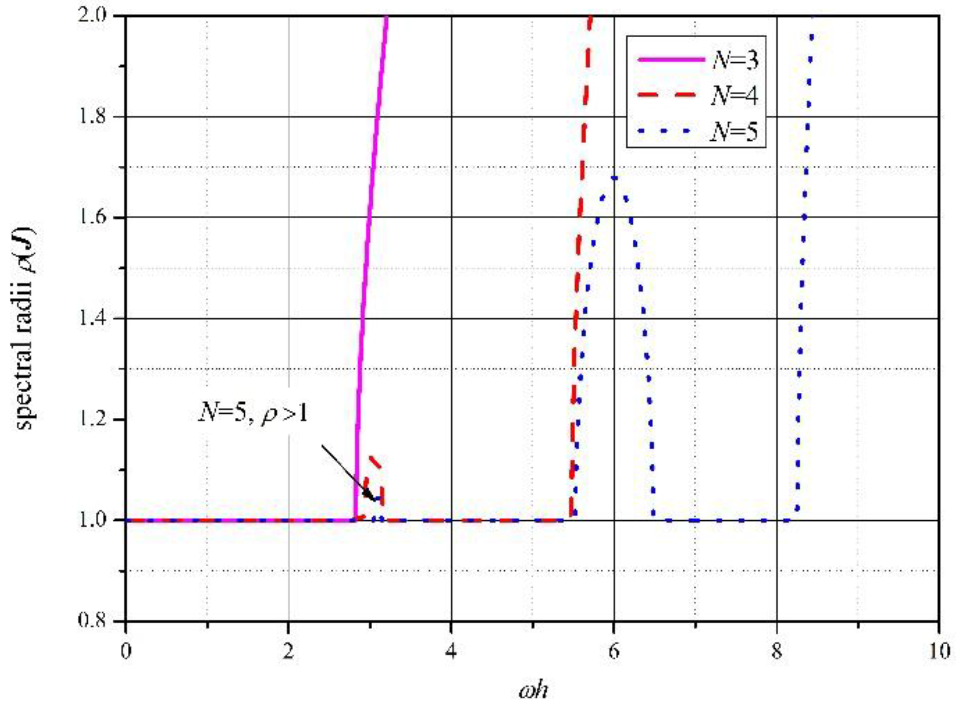
ρ(J) ≥ 1 for any N, and when N becomes larger, the first stable interval also becomes larger. Although there are several stable intervals with ρ(J) = 1 except for N = 3, the first stable interval is significant and practical; therefore, only the first intervals are listed in Table 1 whose elements are obtained by using the criterion (ρ − 1) < 10⁻⁶.

(2)

ρ(J) < 1 in the TFEM by Hulbert [35], but ρ(J) = 1 in DQTFEM for all stable intervals, hence DQTFEM is more accurate than that of Hulbert [35] since DQTFEM is a high-order method that has a smaller phase error than lower order methods. Note that the stability of CDM is ωh ≤ 2, and $\omega h\le 2\sqrt{2}$ for four-order explicit RKM, and the stability of the present method is $\omega h\le 2\sqrt{2}$.

(3)

DQTFEM is highly symplectic. If the Jacobi matrix J of a method satisfies Equation (35) as follows

$$\{\begin{array}{c}\begin{array}{ccc}{\mathit{J}}_1={\mathit{J}}_{11}{\mathit{J}}_{22}^{\mathrm{T}}-{\mathit{J}}_{12}{\mathit{J}}_{21}^{\mathrm{T}}=\mathit{I}& ,& {\mathit{J}}_2={\mathit{J}}_{11}^{\mathrm{T}}{\mathit{J}}_{22}-{\mathit{J}}_{21}^{\mathrm{T}}{\mathit{J}}_{12}=\mathit{I}\end{array}\\ \begin{array}{ccc}{\mathit{J}}_3={\mathit{J}}_{11}^{\mathrm{T}}{\mathit{J}}_{21}-{\mathit{J}}_{21}^{\mathrm{T}}{\mathit{J}}_{11}=\mathbf{0}& ,& {\mathit{J}}_4={\mathit{J}}_{12}^{\mathrm{T}}{\mathit{J}}_{22}-{\mathit{J}}_{22}^{\mathrm{T}}{\mathit{J}}_{12}=\mathbf{0}\end{array}\\ \begin{array}{ccc}{\mathit{J}}_5={\mathit{J}}_{11}{\mathit{J}}_{12}^{\mathrm{T}}-{\mathit{J}}_{12}{\mathit{J}}_{11}^{\mathrm{T}}=\mathbf{0}& ,& {\mathit{J}}_6={\mathit{J}}_{21}{\mathit{J}}_{22}^{\mathrm{T}}-{\mathit{J}}_{22}{\mathit{J}}_{21}^{\mathrm{T}}=\mathbf{0}\end{array}\end{array},$$

(35)

then the method is symplectic. For the present single DOF system, all variables in Equation (35) are numbers and

Table 2. Precision of J₁~J₆, |J| and ρ(J).

(N, max(ωh))	abs(J1 − 1)	abs(J2 − 1)	Ji, i = 3, 4, 5, 6	abs(|J| − 1)	abs(ρ(J) − 1)
(3, 2.828)	2.459 × 10−7	2.459 × 10−7	0	2.812 × 10−7	1.486 × 10−9
(4, 2.927)	6.758× 10−8	6.758 × 10−8	0	7.002 × 10−8	4.289 × 10−9
(5, 3.055)	2.817 × 10−8	2.817 × 10−8	0	3.018 × 10−8	1.087 × 10−9
(10, 9.404)	3.648 × 10−10	3.648 × 10−10	0	3.821 × 10−10	1.821 × 10−12
(15, 15.70)	1.085 × 10−10	1.085 × 10−10	0	1.663 × 10−10	7.223 × 10−12
(20, 25.11)	3.345 × 10−10	3.345 × 10−10	0	3.598 × 10−10	4.538 × 10−11
(25, 34.55)	1.784 × 10−8	1.784 × 10−8	0	1.999 × 10−8	6.046 × 10−10
(30, 37.69)	4.586 × 10−6	4.586 × 10−6	0	4.939 × 10−6	7.919 × 10−8
(35, 50.25)	3.882 × 10−6	3.882 × 10−6	0	4.051 × 10−6	6.124 × 10−8

Note: max(ωh) indicates the upper limit of ωh for the first stable interval in Table 1.

shows that the precision of Equation (35) (especially J₃~J₆) is satisfactory, which indicates that DQTFEM is a symplectic method. In fact, we have numerically verified that DQTFEM is symplectic even if it is not stable. For a stable symplectic method, the magnitudes of all eigenvalues of J are equal to 1, therefore all eigenvalues of J of the present method are equal to 1 when it is stable.

4. Numerical Results and Discussion

This section aims at demonstrating the high accuracy and efficiency of DQTFEM by comparing them with RKM and NMA; note that NMA is equivalent to the Euler mid-point symplectic method. To evaluate the relative computational accuracy of the present method, the relative error for all methods is defined as

$$\mathrm{RelErr}=\frac{\left|\mathrm{Exact}-\mathrm{Approximate}\right|}{{\Vert \mathrm{Exact}\Vert }_{\infty }},$$

(36)

where ‘Exact’ denotes the exact solution at each time sampling point, the infinity norm of which denotes the maximum absolute value of a vector, and the elements of this vector are the exact values at all time sampling points; ‘Approximate’ is the result of DQTFEM at each time sampling point.

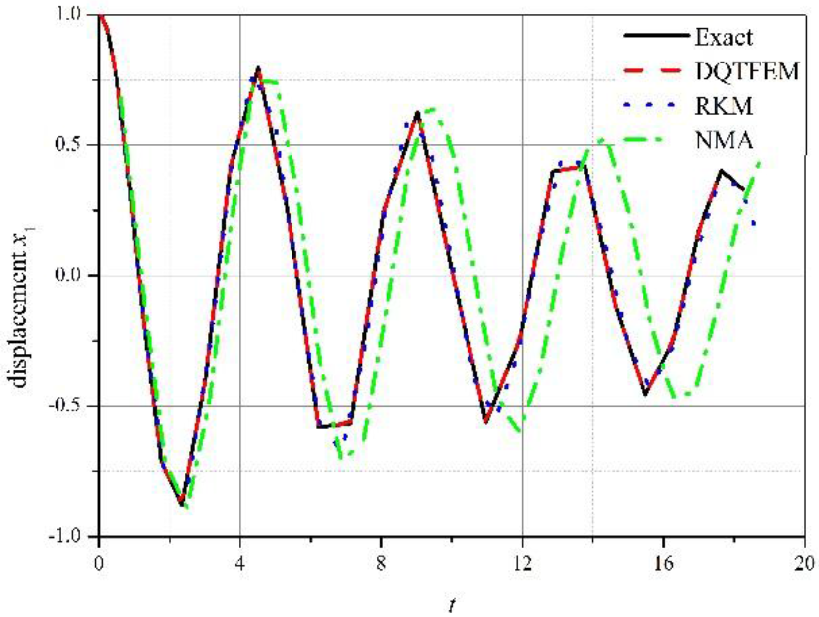
4.1. Free Vibration of a Two-DOF System

Consider the following two-DOF system, its governing equilibrium equation is

$$\left[\begin{array}{cc}2& 0\\ 0& 1\end{array}\right]\left[\begin{array}{c}{\ddot{u}}_1\\ {\ddot{u}}_2\end{array}\right]+\left[\begin{array}{cc}6& -2\\ -2& 4\end{array}\right]\left[\begin{array}{c}{u}_1\\ u_2\end{array}\right]=\left[\begin{array}{c}0\\ 0\end{array}\right],$$

(37)

whose angular frequencies ${\omega }_1=\sqrt{2}$ and ${\omega }_2=\sqrt{5}$. The given initial conditions are $u_0^{\mathrm{T}}=[\begin{array}{cc}1& 1\end{array}]$ and ${\dot{u}}_0^{\mathrm{T}}=\left[0 0\right]$.

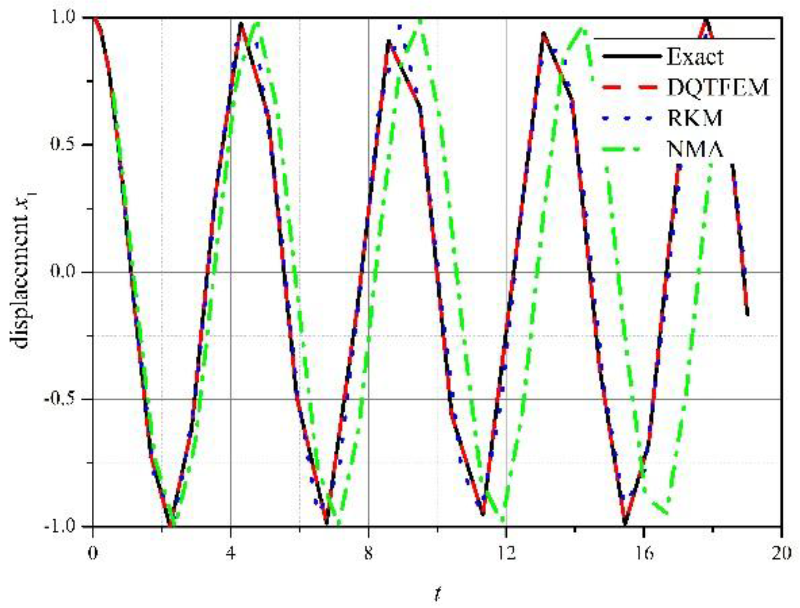
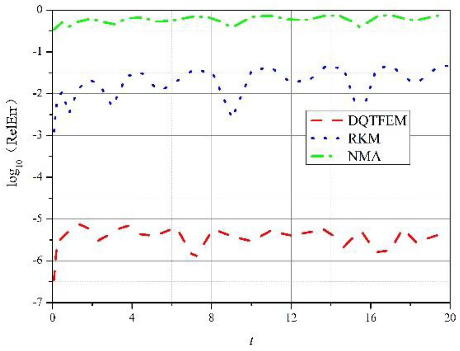
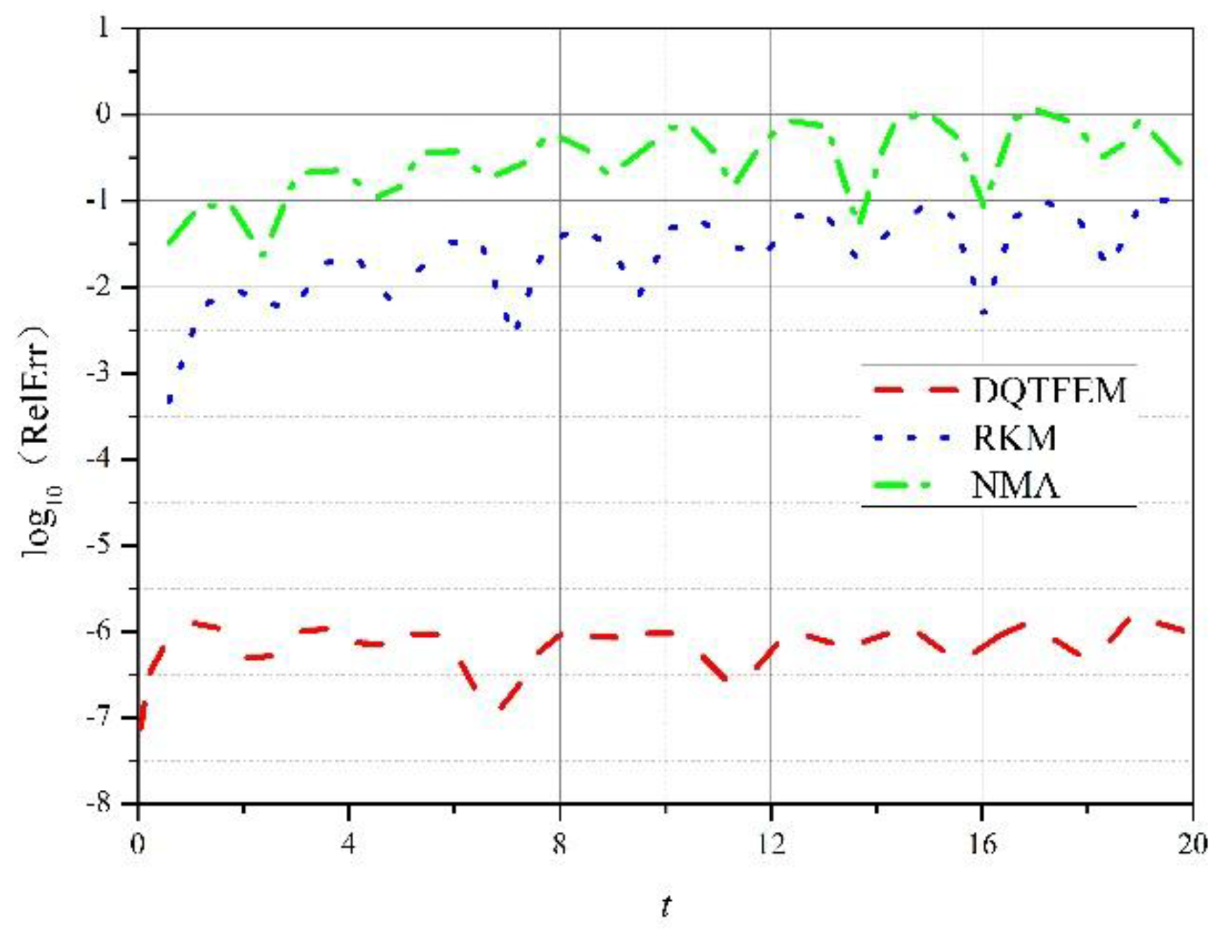
4.1.1. Accuracy Comparison

Let time domain be [0, 19], which is taken as an element with N = 33 non-uniform points in DQTFEM, and 32 uniform time steps are used for both RKM and NMA. The first stable interval for N = 33 is [0, 43.97], hence the stability is satisfied since 19ω₂ = 42.49 < 43.97, and the stability $2\sqrt{2}$ of RKM is also satisfied by h = 19/32 = 0.59375 since ω₂h = 1.3277 < $2\sqrt{2}$. Additionally, N = 33 and h = 0.59375 implies that the three methods have the same number of interpolation points in the domain [0, 19]. The exact solutions used for comparisons are obtained by the mode superposition method.

It follows from Figure 2 and Figure 3 that DQTFEM is much more accurate than RKM and NMA, RelErr (DQTFEM) is about 10⁻⁶, while RelErr (RKM) and RelErr (NMA) are 10⁻² and 10⁻¹, respectively; and it is noticeable from Figure 3 that the errors of RKM and NMA accumulate over time.

4.1.2. Efficiency Comparison

Computational cost is also a crucial issue for a method. Assume the time domain is [0, 2 × 10³] in this case. In order to achieve the same accuracy of RelErr = 10⁻⁶, h = 5 × 10⁻² and h = 1 × 10⁻³ must be used for RKM and NMA, respectively; that is, RKM needs 4 × 10⁵ time steps and NMA needs 2 × 10⁶ time steps. However, we can achieve the same accuracy by using 1588 elements and each element of size h = 1.26 ≈ 2.828/ω₂ has only three Gauss–Lobatto–Legendre sampling points (N = 3 is the least number of time sampling points in an element; see Table 2). If N > 3, the accuracy of DQTFEM is more than 10⁻⁶. For example, if N = 20 in an element of size h = 11 ≈ 25.11/ω₂, the accuracy will be 10⁻⁹. In other words, the lowest accuracy of DQTFEM is 10⁻⁶. This is the reason why the data corresponding to RelErr = 10⁻² are not provided in

Table 3. CPU time comparison.

Method	RelErr = 10−6			RelErr = 10−2
	h	Time Steps	CPU (s)	h	Time Steps	CPU (s)
DQTFEM	1.26	1588	0.4932
RKM	5 × 10−2	4 × 105	4.743	0.32	6.25 × 103	0.7843
NMA	1 × 10−3	2 × 106	249.4	4.5 × 10−2	4.445 × 104	1.184

, which indicates that DQTFEM is much more efficient than the other two methods, especially if high accuracy is required. Another observation is that RKM is more efficient than NMA.

NMA is a symplectic method of second order, in which the amplitude can be rigorously preserved for linear systems, but its phase error is larger than that of RKM. It is well known that dynamic responses must be represented by amplitude and phase together; therefore, RKM is more efficient than NMA for achieving the same accuracy. However, the weakness of RKM is its numerical dissipation and the weakness of NMA is its larger phase error. For long-time kinematics simulations in which only amplitude is taken into account, NMA is a better choice.

4.1.3. Damping Vibration

For further validation of the present method, Rayleigh damping given in Equation (38) is added to the system as Equation (37).

$$C=\left[\begin{array}{cc}0.3& -0.1\\ -0.1& 0.2\end{array}\right]$$

(38)

N = 33 and h = 0.59375 are also used here. The displacement x₁ and RelErr are given in Figure 4 and Figure 5, respectively, from which one can see that DQTFEM is also the most accurate: its RelErr reaches 10⁻⁶. Therefore, the present method is also applicable to the analysis of damped problems.

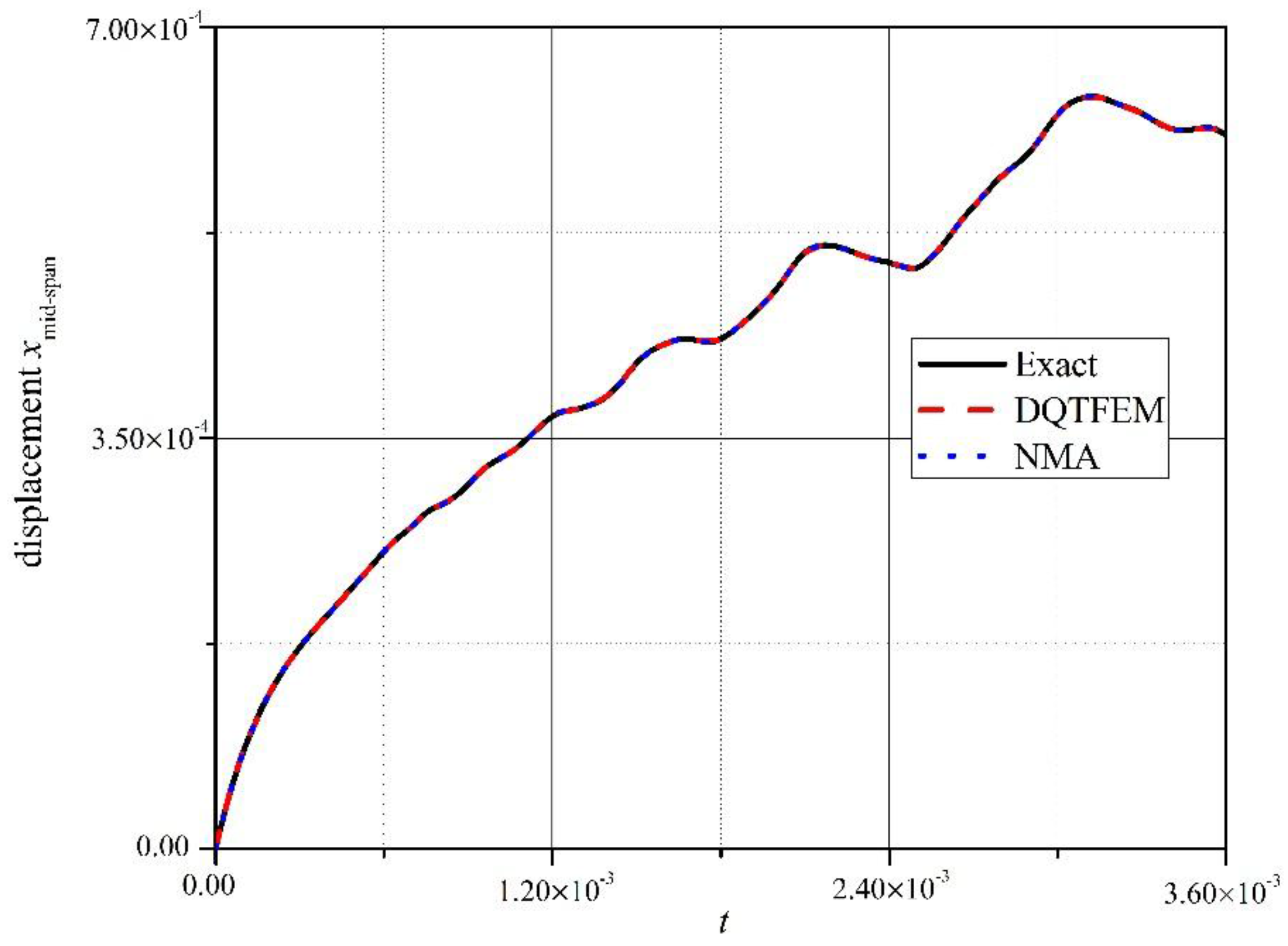
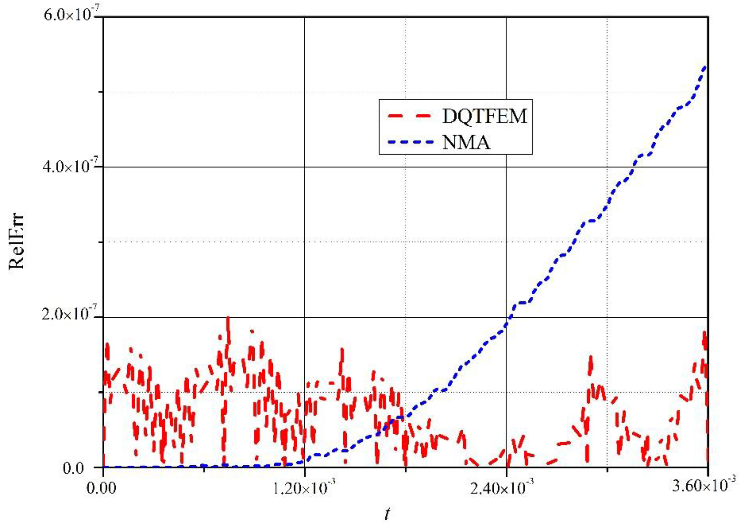
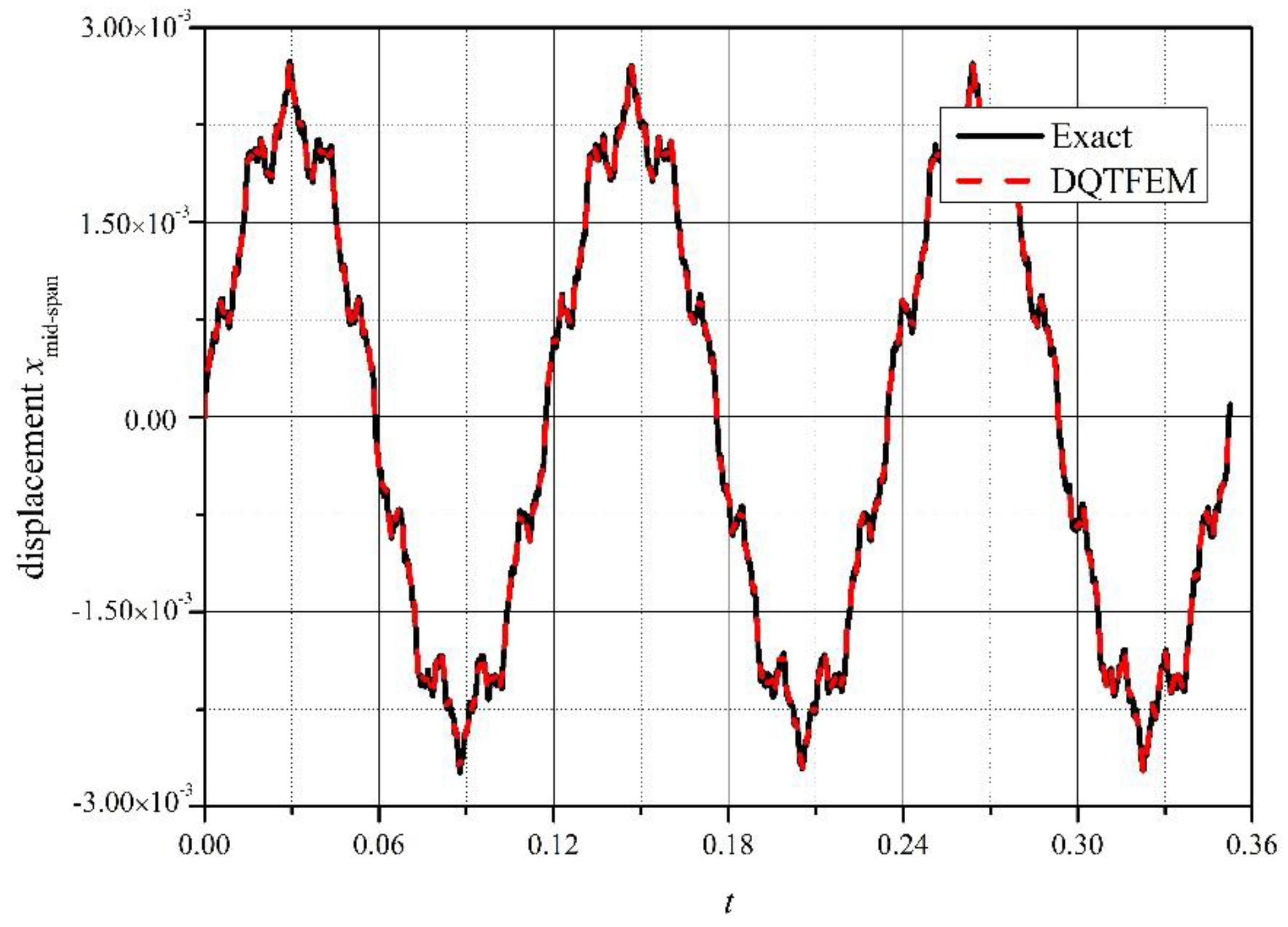
4.2. Free Vibration of a Simply Supported Euler Beam

In order to further explore the accuracy and efficiency of DQTFEM, the free vibration of a simply supported Euler beam of length L = 3 m is studied in this section; flexural rigidity EI = 1 × 10⁶ N/m and mass density per unit length ρA = 420 kg/m. The beam is meshed into 16 uniform cubic elements. All initial velocities and displacements are equal to zero except the initial velocity at mid-span is 1 m/s; apparently the problem is analogous to the impact problem.

Consider time domain [0, 3.6 × 10⁻³] s, which is meshed into 10 uniform time elements, that is h = 3.6 × 10⁻⁴ s, and 20 Gauss–Lobatto–Legendre sampling points are involved in each element. Note that, if the highest frequency is ω₃₃ = 6.967 × 10⁴ rad/s, then ω₃₃h = 25.08 falls into the first stable interval 0 < ωh ≤ 25.11 for N = 20; see Table 1.

Figure 6 shows an excellent agreement of DQTFEM with the exact method. For reaching the same order of accuracy, NMA needs 2.110 × 10⁵ time steps and much more CPU time than DQTFEM; see

Table 4. CPU time comparison between DQTFEM and NMA (RelErr = 10⁻⁷).

Method	h (s)	Time Steps	CPU (s)
DQTFEM	3.6 × 10−4	10	0.9376
NMA	1.706 × 10−8	2.110 × 105	294.8

. Figure 7 presents the RelErr comparisons between DQTFEM and NMA; it follows that the error of NMA accumulates while the error of DQTFEM does not.

For validating the effectiveness of DQTFEM for long-term simulation, the computational time changes from 3.6 × 10⁻³ s to three times the maximum period T_max = 2π/ω₁ = 0.1174 s, where ω₁ = 53.51 rad/s, the number of elements is 3T_max/h ≈ 978. Figure 8 gives a comparison of displacements by DQTFEM with the exact solution, which shows that DQTFEM is also highly accurate for this case and the needed CPU time is only 75.53 s. Nevertheless, the NMA results are not presented since NMA requires a prohibitively long CPU time.

5. Conclusions

A highly accurate and highly efficient DQTFEM was developed in the present study by using the DQ rule, the Gauss–Lobatto integration rule, and the general form of Hamilton’s variational principle for solving structural dynamic problems involving damping and external forces.

DQTFEM incorporates the high accuracy and efficiency of DQM into the development of high-order time elements, in which initial conditions can be introduced in the same simple and general form as in standard FEM. Furthermore, DQTFEM can serve as a step-by-step approach; one time element of DQTFEM can be seen as one time step of the conventional step-by-step method. Moreover, it has been shown that DQTFEM is a highly accurate symplectic method.

Extensive numerical comparisons validated the present method, whose solutions can be seen as benchmarks to validate lower-order DIMs and TFEMs. It is expected that DQTFEM will be practical in the future.

References

1. Feng, K. Difference schemes for hamiltonian formalism and symplectic geometry. J. Comput. Math. 1986, 4, 279–289. [Google Scholar]
2. Zienkiewicz, O.C. A new look at the newmark, houbolt and other time stepping formulas. A weighted residual approach. Earthq. Eng. Struct. Dyn. 1977, 5, 413–419. [Google Scholar] [CrossRef]
3. Argyris, J.H.; Scharpf, D.W. Finite elements in time and space. Nucl. Eng. Des. 1969, 10, 456–464. [Google Scholar] [CrossRef]
4. Fried, I. Finite element analysis of time dependent phenomena. AIAA J. 1969, 7, 1170–1173. [Google Scholar] [CrossRef]
5. Tang, W.S.; Sun, Y.J. Time finite element methods: A unified framework for numerical discretizations of odes. Appl. Math. Comput. 2012, 219, 2158–2180. [Google Scholar] [CrossRef]
6. Simkins, T.E. Finite elements for initial value problems in dynamics. AIAA J. 1981, 19, 1357–1362. [Google Scholar] [CrossRef]
7. Brugnano, L.; Iavernaro, F.; Trigiante, D. A simple framework for the derivation and analysis of effective one-step methods for odes. Appl. Math. Comput. 2012, 218, 8475–8486. [Google Scholar] [CrossRef]
8. Wilson, E.L.; Nickell, R.E. Application of the finite element method to heat conduction analysis. Nucl. Eng. Des. 1966, 4, 276–287. [Google Scholar] [CrossRef]
9. Zienkiewicz, O.C.; Wood, W.L.; Hine, N.W.; Taylor, R.L. A unified set of single step algorithms. Part 1: General formulation and applications. Int. J. Numer. Methods Eng. 1984, 20, 1529–1553. [Google Scholar] [CrossRef]
10. Richter, T.; Wick, T. Variational localizations of the dual weighted residual estimator. J. Comput. Appl. Math. 2015, 279, 192–209. [Google Scholar] [CrossRef]
11. Ma, L.M.; He, Y.A. A single-step time element method for dynamic response by gurtin variational principle. Eng. Mech. 1995, 12, 24–29. [Google Scholar]
12. Zhong, W.; Yao, Z. Time domain fem and symplectic conservation. J. Mech. Strength 2005, 27, 178–183. [Google Scholar]
13. Ding, X.C.; Chen, Q.W. Subinterval method for direct calculation of response of dynamic system by using hamilton’s principle. Earthq. Eng. Eng. Vib. 1987, 7, 9–19. [Google Scholar]
14. Tung, M.M.; Defez, E.; Sastre, J. Numerical solutions of second-order matrix models using cubic-matrix splines. Comput. Math. Appl. 2008, 56, 2561–2571. [Google Scholar] [CrossRef]
15. Bellour, A.; Sbibih, D.; Zidna, A. Two cubic spline methods for solving fredholm integral equations. Appl. Math. Comput. 2016, 276, 1–12. [Google Scholar] [CrossRef]
16. Givoli, D.; Hagstrom, T.; Patlashenko, I. Finite element formulation with high-order absorbing boundary conditions for time-dependent waves. Comput. Methods Appl. Mech. Eng. 2006, 195, 3666–3691. [Google Scholar] [CrossRef]
17. Jiang, Y.J.; Ma, J.T. High-order finite element methods for time-fractional partial differential equations. J. Comput. Appl. Math. 2011, 235, 3285–3291. [Google Scholar] [CrossRef]
18. Krishna, M.S.; Manjeet, S.K. Three and four step least square finite element schemes in the time domain. Commun. Numer. Methods Eng. 1996, 12, 425–432. [Google Scholar]
19. Jiwari, R. Lagrange interpolation and modified cubic b-spline differential quadrature methods for solving hyperbolic partial differential equations with dirichlet and neumann boundary conditions. Comput. Phys. Commun. 2015, 193, 55–66. [Google Scholar] [CrossRef]
20. Kawahara, M.; Hasegawa, K. Periodic galerkin finite element method of tidal flow. Int. J. Numer. Methods Eng. 1978, 12, 115–128. [Google Scholar] [CrossRef]
21. Jia, Z.; Cheng, X.; Zhao, M. A new method for roots of monic quaternionic quadratic polynomial. Comput. Math. Appl. 2009, 9, 1852–1859. [Google Scholar] [CrossRef]
22. Hoff, C.; Hughes, T.J.R.; Hulbert, G.; Pahl, P.J. Extended comparison of the hilber-hughes-taylor α-method and the θ1-method. Comput. Methods Appl. Mech. Eng. 1989, 76, 87–94. [Google Scholar] [CrossRef]
23. Chang, J.C. Combining genetic algorithm and taylor series expansion approach for doa estimation in space-time cdma systems. Appl. Soft Comput. J. 2015, 28, 208–217. [Google Scholar] [CrossRef]
24. Khan, I.R.; Ohba, R.; Hozumi, N. Mathematical proof of closed form expressions for finite difference approximations based on taylor series. J. Comput. Appl. Math. 2003, 150, 303–310. [Google Scholar] [CrossRef]
25. Hoff, C.; Pahl, P.J. Practical performance of the θ1-method and comparison with other dissipative algorithms in structural dynamics. Comput. Methods Appl. Mech. Eng. 1988, 67, 87–111. [Google Scholar] [CrossRef]
26. Reed, W.H.; Hill, T.R. Triangular Mesh Methods for the Neutron Transport Equation; Los Alamos Scientific Laboratory: Los Alamos, NM, USA, 1973. [Google Scholar]
27. Lasaint, P.; Raviart, P.A. On a finite element method for solving the neutron transport equation. In Mathematical Aspects of Finite Elements in Partial Differential Equations, Proceedings of a Symposium Conducted by the Mathematics Research Center, the University of Wisconsin-Madison, Madison, WI, USA, 1–3 April, 1974; Elsevier: Amsterdam, The Netherlands, 1974; Volume 56, pp. 89–124. [Google Scholar]
28. Gudla, P.K.; Ganguli, R. Discontinuous galerkin finite element in time for solving periodic differential equations. Comput. Methods Appl. Mech. Eng. 2006, 196, 682–697. [Google Scholar] [CrossRef]
29. Gao, Y.L.; Mei, L.Q.; Li, R. A time-splitting galerkin finite element method for the davey-stewartson equations. Comput. Phys. Commun. 2015, 197, 35–43. [Google Scholar] [CrossRef]
30. Delfour, M.; Hager, W.; Trochu, F. Discontinuous galerkin methods for ordinary differential equations. Math. Comput. 1981, 36, 455–474. [Google Scholar] [CrossRef]
31. Hughes, T.J.R.; Hulbert, G.M. Space-time finite element methods for elastodynamics: Formulations and error estimates. Comput. Methods Appl. Mech. Eng. 1988, 66, 339–364. [Google Scholar] [CrossRef]
32. Hulbert, G.M.; Hughes, T.J.R. Space-time finite element methods for second-order hyperbolic equations. Comput. Methods Appl. Mech. Eng. 1990, 84, 327–349. [Google Scholar] [CrossRef]
33. Chessa, J.; Belytschko, T. A local space–time discontinuous finite element method. Comput. Methods Appl. Mech. Eng. 2006, 195, 1325–1344. [Google Scholar] [CrossRef]
34. Dyniewicz, B. Space-time finite element approach to general description of a moving inertial load. Finite Elem. Anal. Des. 2012, 62, 8–18. [Google Scholar] [CrossRef]
35. Hulbert, G.M. Time finite element methods for structural dynamics. Int. J. Numer. Methods Eng. 1992, 33, 307–331. [Google Scholar] [CrossRef]
36. Nam, J.; Behr, M.; Pasquali, M. Space-time least-squares finite element method for convection-reaction system with transformed variables. Comput. Methods Appl. Mech. Eng. 2011, 200, 2562–2577. [Google Scholar] [CrossRef] [PubMed]
37. Chien, C.C.; Wu, T.Y. An improved predictor/multi-corrector algorithm for a time-discontinuous galerkin finite element method in structural dynamics. Comput. Mech. 2000, 25, 430–438. [Google Scholar] [CrossRef]
38. Aubry, D.; Lucas, D.; Tie, B. Adaptive strategy for transient/coupled problems applications to thermoelasticity and elastodynamics. Comput. Methods Appl. Mech. Eng. 1999, 1, 41–51. [Google Scholar] [CrossRef]
39. Larsson, F.; Hansbo, P.; Runesson, K. Space-time finite elements and an adaptive strategy for the coupled thermoelasticity problem. Int. J. Numer. Methods Eng. 2003, 56, 261–294. [Google Scholar] [CrossRef]
40. Bellman, R.; Casti, J. Differential quadrature and long-term integration. J. Math. Anal. Appl. 1971, 34, 235–239. [Google Scholar] [CrossRef]
41. Shu, C. Differential Quadrature and Its Application in Engineering; Springer: London, UK, 2000. [Google Scholar]
42. Eftekhari, S.A.; Khani, M. A coupled finite element-differential quadrature element method and its accuracy for moving load problem. Appl. Math. Model. 2010, 34, 228–238. [Google Scholar] [CrossRef]
43. Eftekhari, S.A.; Jafari, A.A. Mixed finite element and differential quadrature method for free and forced vibration and buckling analysis of rectangular plates. Appl. Math. Mech. 2012, 33, 81–98. [Google Scholar] [CrossRef]
44. Wang, X.; Yuan, Z. Harmonic differential quadrature analysis of soft-core sandwich panels under locally distributed loads. Appl. Sci. 2016, 6, 361. [Google Scholar] [CrossRef]
45. Tornabene, F.; Fantuzzi, N.; Ubertini, F.; Viola, E. Strong formulation finite element method based on differential quadrature: A survey. Appl. Mech. Rev. 2015, 1, 145–175. [Google Scholar] [CrossRef]
46. Bert, C.W.; Malik, M. Differential quadrature method in computational mechanics: A review. Appl. Mech. Rev. 1996, 49, 1–29. [Google Scholar] [CrossRef]
47. Xing, Y.; Liu, B. High-accuracy differential quadrature finite element method and its application to free vibrations of thin plate with curvilinear domain. Int. J. Numer. Methods Eng. 2009, 80, 1718–1743. [Google Scholar] [CrossRef]
48. Xing, Y.F.; Liu, B.; Liu, G. A differential quadrature finite element method. Int. J. Appl. Mech. 2012, 2, 207–227. [Google Scholar] [CrossRef]
49. Reddy, J.N. Energy and Variational Methods in Applied Mechanics; John Wiley & Sons: New York, NY, USA, 1984. [Google Scholar]
50. Fung, T.C. Solving initial value problems by differential quadrature method-part 1: First-order equations. Int. J. Numer. Methods Eng. 2001, 50, 1411–1428. [Google Scholar] [CrossRef]
51. Bartels, R.H.; Stewart, G.W. Solution of the matrix equation ax + xb = c. Commun. ACM 1972, 15, 820–826. [Google Scholar] [CrossRef]
Figure 1. Spectral radii for different N.
Applsci 07 00138 g001
Figure 2. Comparisons of displacement x1 (N = 33, h = 0.59375).
Applsci 07 00138 g002
Figure 3. RelErr comparisons (N = 33, h = 0.59375).
Applsci 07 00138 g003
Figure 4. Displacement comparison for damping case (N = 33, h = 0.59375).
Applsci 07 00138 g004
Figure 5. RelErr for damping case (N = 33, h = 0.59375).
Applsci 07 00138 g005
Figure 6. Displacement comparison of beam.
Applsci 07 00138 g006
Figure 7. RelErr comparison between DQTFEM and NMA for xmid-span.
Applsci 07 00138 g007
Figure 8. Displacement comparison for long-term simulation.
Applsci 07 00138 g008