CFD Studies of the Effects of Waveform on Swimming Performance of Carangiform Fish

Abstract

Carangiform fish, like mackerel, saithe and bass, swim forward by rhythmically passing body waves from the head to the tail. In this paper, the undulating motions are decomposed into the travelling part and the standing part by complex orthogonal decomposition (COD), and the ratio between these two parts, i.e., the travelling index, is proposed to analyse the waveform of fish-like movements. To further study the relative influences of the waveform on swimming performance, a self-propelled model of carangiform fish is developed by the level set/immersed boundary (LS-IB) method, and the in-house code is tested by two cases of flow past a sphere and an oscillating cylinder, respectively. In this study, the travelling index is varied in ranges up to 50% larger or smaller than the biological data. The results show that carangiform fish seem to favour a fast and efficient swimming motion with a travelling index of around 0.6. Meanwhile, we study several numerical cases with different amplitude coefficients (0.5~1.1) and tail-beat frequency (2 Hz~5 Hz), and then compare their swimming performance with each other. We found that the forward speed is closely related to the travelling index and tail-beat frequency, while the swimming efficiency is increased with the tail-beat frequency and amplitude coefficient. These results are also consistent with biological observations, and they might provide beneficial guidance with respect to the future design of robotic fish.

1. Introduction

After millions of years of evolution, fish have evolved with extremely excellent propulsive capabilities, which are far superior to those of man-made watercrafts. In nature, most fish primarily use body and/or caudal fin (BCF) to generate thrust. Based on the fraction of their body that is displaced laterally, they can be subdivided into anguilliform, subcarangiform, carangiform and thunniform modes [1]. As exhibited by, for example, saithe, mackerel and bass, carangiform fish have a streamlined body with a homocercal caudal fin. Their undulations are mostly restricted to the posterior half or even third of the body, and the amplitude increases sharply in the caudal area. As suggested by Videler [2], the fish-like movement is described by the approximate trajectory of midline motion $h\left(x,t\right)$, which is identified by a sinusoidal travelling wave with an increasing amplitude envelope. It is expressed as:

$$h\left(x,t\right)=\left(a_1+a_{2}x+a_3{x}^2\right)\sin \left(\mathsf{\omega }t-kx\right)$$

(1)

where $h\left(x,t\right)$ represents the midline motion of fish body; $\mathsf{\omega }$ is the tail-beat frequency; $k=2\mathsf{\pi }/\mathsf{\lambda }$ is the wave number, $\mathsf{\lambda }$ is the wave length; $a_1$, $a_2$ and $a_3$ are the quadratic coefficients of the amplitude envelope.

In reality, the midline motions of fish body are closely related to swimming performance. However, the effects of waveform on the propulsive performance are often contradictory. Similar to the airfoil, the influence might be explained by the net force caused by the body movements. For example, Barrett et al. [3] built a physical fish-like bio-robot, and concluded that the undulatory motion may result in a reduction in drag. However, Lighthill’s analytical results [4] indicate that the friction drag increases with the undulatory motion, which was also verified by the experiments of Anderson et al. [5]. The issue of whether undulatory motion is drag-reducing or drag-increasing is still a debate in the literature. In this paper, we applied the method of complex orthogonal decomposition (COD) to analyse the movements of carangiform fish. The midline motions are decomposed into the standing and travelling parts, and the ratio between the travelling part and standing part is defined as the travelling index [6,7]. In contrast to Feeny’s work [7], we analysed the effects of travelling index on the swimming performance in terms of the forward speed and swimming efficiency.

So far, the influences of fish-like motions on the propulsive performance have been explored by biological experiments [2], robotic fish [3] and by numerical simulations [8,9,10,11]. By comparison, the body movements in both the biological experiments and the robotic fish cannot be controlled as desired. However, the numerical simulations offer an effective tool to model the swimming fish with any described motions, and the flow characteristics and hydrodynamic force can be also calculated simultaneously. For example, Carling [8] and Tian [10,11] built a self-propelled fish model which swam in viscous flow, using the finite difference method and the finite element method, respectively. Borazjani and Sotiropoulos [9] use the curvilinear-immersed boundary (IB) method to investigate the influences of the body shape and midline motions on the swimming performance of a mackerel fish. In our work, the hybrid Cartesian immersed boundary method [12,13] is used, which is suitable to deal with the deformed solid body. All the Cartesian grid points are split into the fluid points, the solid points, and the forcing points. The forcing points are the grid points in the fluid phase with one or more neighbouring points in the solid phase. The velocities at the forcing points are reconstructed via the known boundary values on the surface of solid body and the information from the interior flow.

Traditionally, the Lagrange girds are generated on the surface of solid body to identify the velocity of the solid points [13,14]. In contrast, the level set (LS) function ϕ is defined as a signed distance to the fluid-solid interface, of which the value is positive and negative in the fluids and solid bodies, respectively. The fluid–solid interface is defined as the iso-contour ϕ = 0, determined by the geometry of the solid body. Most importantly, we use LS function to identify and track the normal direction of solid points on the surface of solid body. This is totally different from the traditional approach [14], in which the solid/fluid nodes around the interface are used. In contrast, Cheny et al. [15] and Meyer et al. [16] used the LS function to track the solid–fluid interface, but they used the cut-cell methods to solve the transient fluid flow, with the drawbacks of small time step and gird size. In this study, a modified LS-based Cartesian-IB method is developed to simulate the interactions between fluid flows and the deformed fish body. For the self-propelled model, the midline motions of carangiform fish are described, and the LS function needs to be regenerated at every time step. In contrast to the numerical method in reference [17], the reinitialization procedure is used to fix the LS function of the fish body, rather than solving the LS function.

In this study, the travelling index of the midline motion, as well as the amplitude and tail-beat frequency, is changed to be up to 50% larger or smaller than the biological value. Their influences on swimming performance are evaluated by the forward speed and swimming efficiency. Overall, the major contributions of the present work are: (1) development of a modified LS-IBM method to simulate the swimming fish; and (2) use of the travelling index to investigate the influences of the fish-like motions on their swimming performance. This paper is organized as follows: the problem definition of carangiform swimmers and numerical method are given in Section 2 and Section 3, respectively, Section 4 presents the simulation results, and Section 5 and Section 6 show the discussion and conclusions, respectively.

2. Physical Problems of Carangiform Fish

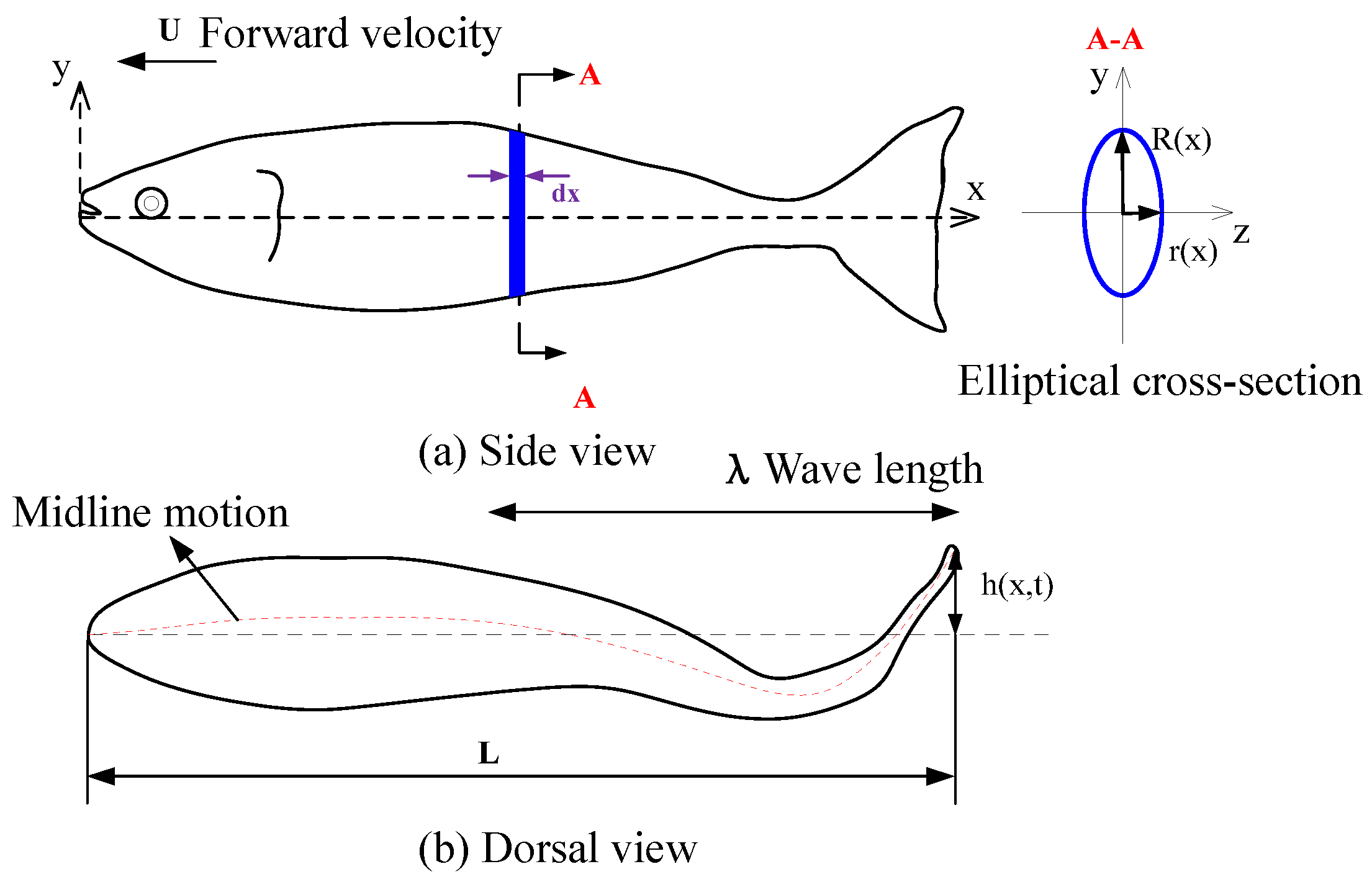
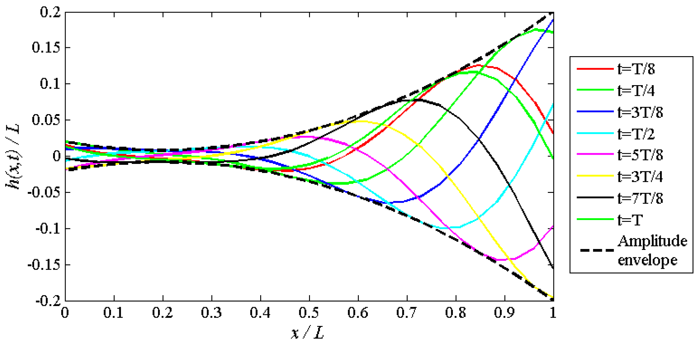
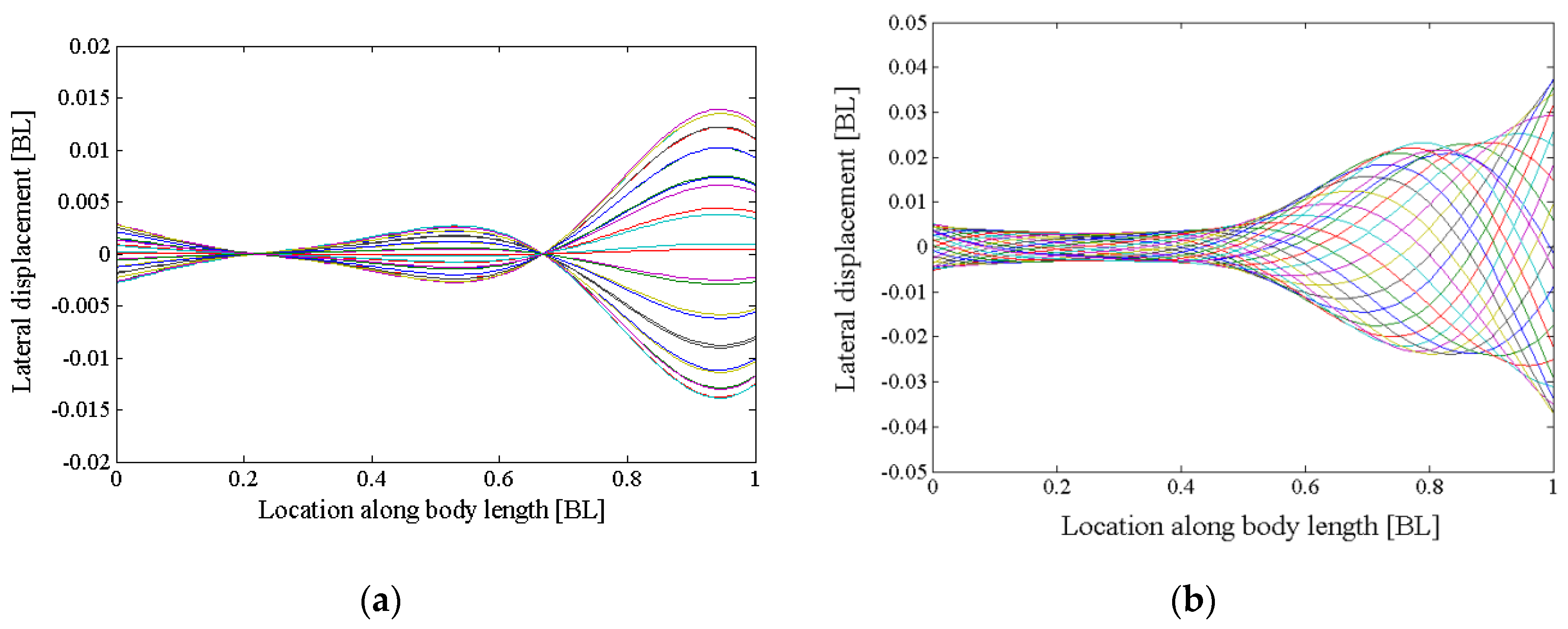
2.1. Shape and Kinematic Parametrization

As shown in Figure 1, the cross-section of carangiform fish can be defined as an ellipse, and the profiles of the half-height $R\left(x\right)$ and the half-width $r\left(x\right)$ are expressed as [18]:

$$R\left(x\right)=0.14L\sin \left(2\mathsf{\pi }x/1.6L\right)+0.0008L(e^{2\mathsf{\pi }x/1.1L}-1)$$

(2)

$$r\left(x\right)=0.045L\sin \left(2\mathsf{\pi }x/1.25L\right)+0.06L\sin \left(2\mathsf{\pi }x/3.14L\right)$$

(3)

where $L$ is the full length of fish body.

For carangiform fish, Alvarado [18] summarized a set of kinematic parameters to describe their midline motions, which are scaled by the full length of the fish body. In detail, the biological parameters are $k=7.0/L$, $a_1=0.004fL$, $a_2=-0.02f$ and $a_3=0.04f/L$; $f$ is the tail-beat frequency. When the tail-beat frequency is 2 Hz, the midline motions in a full undulation cycle are shown in Figure 2.

2.2. Self-Propelled Fish Model

In our simulations, the computational domain size in the length and width directions is $35L\times 4L$, and the number of grid points is 2560 × 256, respectively. The domain width is 59.7 times the maximum width of fish body ($0.067L$). The mesh is uniform in the length direction, and the mesh in the width direction is stretched from the centreline to the boundaries using a hyperbolic tangent function. Initially, the fish model is placed $0.5L$ from the inlet plane, and centred in the vertical direction. The grid size near fish body is $0.0028L\times 0.0028L$, and the CFL (Courant-Friedrichs-Lewy) number is 0.5. The outer boundary conditions used are as following: the uniform flow at the inlet plane, slip wall condition at the lateral boundaries, and Neumann boundary condition at the outlet.

For the self-propelled fish model, the swimming motion is governed by Newton’s equations:

$$m_f\frac{{\partial }^2{x}_c}{\partial t^2}=F_f$$

(4)

where $m_f$ is the mass of fish body; $x_c$ represents the position of the mass centre; and $F_f$ is the net force around fish body. In the simulations, the virtual fish is initially placed in the stagnant fluid, and starts to undulate its body with the described motions. Due to body undulations, a thrust force is exerted by the flow, which accelerates the virtual fish to higher velocities. At the same time, the drag force is increased with the forward speed, until it balances with the thrust force during a tail-beat period. Thereafter, the virtual fish reaches a quasi-steady state with a constant average velocity.

2.3. Evaluations of Swimming Performance

As known, the swimming abilities of carangiform fish are varied with the midline motions. Therefore, several parameters are used to quantify the swimming performance, and listed as:

(1) Travelling index

The travelling index was firstly proposed by Feeny [6]. For the sake of completeness, we briefly introduce the concept of travelling index here. Similar to the work of Feeny et al. [7], the method of complex orthogonal decomposition (COD) is used to decompose the midline motions of the fish. To conduct the COD analysis of the swimming motions, we first generate a matrix:

$$Y_{\mathrm{M}\times \mathrm{N}}={\left[y_1\left(t_n\right),y_1\left(t_n\right),\dots \dots ,y_{\mathrm{N}}\left(t_n\right)\right]}^{\mathrm{T}}=\mathrm{h}\left(x_m,t_n\right)$$

(5)

In Equation (5), the component at row m and column n of matrix $Y$ represents the transverse displacement of the fish midline at marker point x_m (for m = 1, 2, … M) and time t_n (for n = 1, 2… N). The marker points x_m are evenly spaced along the fish midline as x_m = mL/M, and the time instants t_n are also uniformly sampled inside a tail-beat period as t_n = nT/N. A complex matrix $Z_{M\times N}={\left[z_1\left(t_n\right), z_1\left(t_n\right), \dots \dots , z_N\left(t_n\right)\right]}^{\mathrm{T}}$ is then built based on matrix $Y$. Here, z_m(t) = y_m(t) + iH(y_m(t)) is the analytical vector of y_m, where $\mathrm{i}$ represents the imaginary unit and H(y_m(t)) is the Hilbert transform of y_m(t). A complex correlation matrix $R=Z{\overline{Z}}^{\mathrm{T}}/N$ is then generated, where the overbar indicates the conjugation of a complex number. Matrix $R_{M\times M}$ is a complex Hermitian matrix, which has real eigenvalues ${\mathsf{\lambda }}_m$ and complex eigenvectors $w_m$. The travelling index $\alpha$ is then calculated as:

$$\alpha =1/\mathrm{cond}\left(W\right)$$

(6)

where $W=\left[\mathrm{real}\left(w_1\right),\mathrm{imag}\left(w_1\right)\right]$ is a matrix with its two columns being the real and imaginary part of w, and cond(W) denotes condition number of matrix W. The value of the travelling index equates the reciprocal of the relative condition number, which represents the relative ratio between the travelling and standing components. In particular, when the value of travelling index equates zero, this means there is no independence between the real and imaginary vectors, thus it is a pure standing wave. When the travelling index is 1.0, it indicates complete independence between the two vectors, and the wave is a “fully” travelling wave.

(2) Reynolds number

In the field of fish propulsion, the Reynolds number is a dimensionless parameter that is used to describe the fluid environment. For the self-propelled fish model, the Reynolds number is defined as:

$${\mathrm{Re}}_f=L^2/\left(T\nu \right)$$

(7)

where $T=1/f$ is the beating period, and $\nu$ is the kinematic viscosity. In our cases, we set the viscosity of the fluid to be 6.25 × 10⁻⁴ (N·s)/m², the beating period $T=0.4 \mathrm{s}$, and the length of fish body is 1 m, resulting in a Reynolds number of 4000.

(3) Strouhal number

In swimming fish, the Strouhal number is defined as:

$$St=f{A}_{max}/U$$

(8)

where $A_{max}$ is the maximum amplitude of fish tail, and $U$ is the forward velocity. For real fish, Taylor et al. [19] suggested that the St number has an optimal range, ranging from 0.25 to 0.35.

(4) Swimming efficiency

For the self-propelled fish model, the swimming efficiency is defined as the ratio of useful work over the total energy. In present study, the quasi-propulsive efficiency [20] is adopted to quantify the swimming efficiency. It is defined as the ratio of the power required to tow the fish body in a rigid and straight manner over the power used for self-propulsion with the same speed, which is given by:

$${\mathsf{\eta }}_{\mathrm{QP}}=\frac{RU}{P_{in}}$$

(9)

where $U$ is the forward speed at the quasi-steady state; $R$ is the resistance force of the rigid-straight towed body at the speed $U$; and $P_{in}$ is the required power to drive the virtual fish at the speed $U$.

3. Numerical Methods

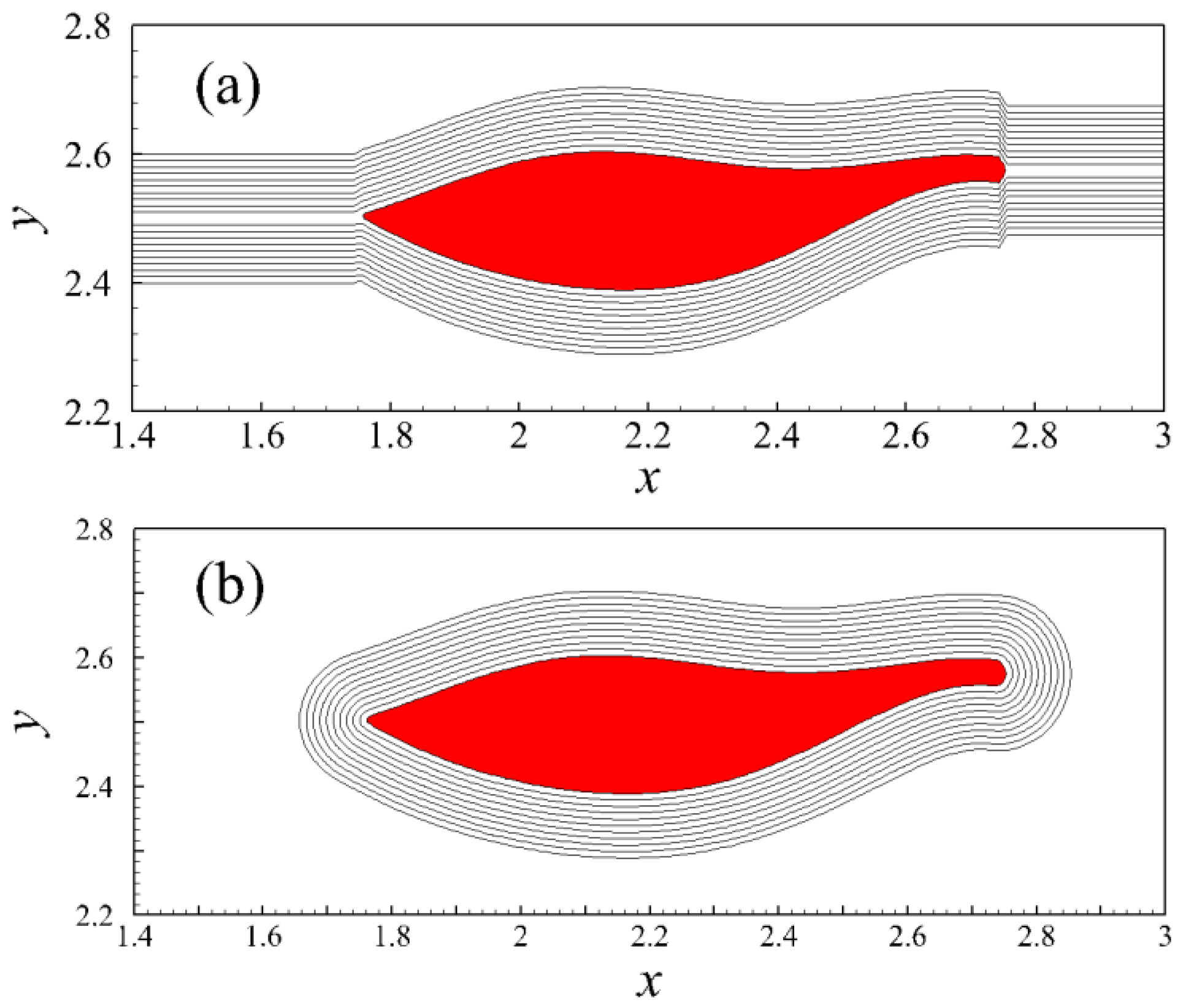
3.1. Level Set Function

The level set (LS) function has been widely used in applications, such as in breaking waves, bubble dynamics, and computer graphics [21]. In this study, the LS function is used to describe the fluid–solid interface:

$$\mathsf{\varphi }(\overrightarrow{x},t)=\{\begin{array}{c}-\mathsf{\Gamma }\left(\overrightarrow{x},t\right)insolid\\ 0interface\\ \mathsf{\Gamma }\left(\overrightarrow{x},t\right)influid\end{array}$$

(10)

where $\mathsf{\Gamma }$ is the distance from any point to the fluid–solid interface. The points on the fluid–solid boundary have $\mathsf{\varphi }(\overrightarrow{x},t)=0$. For example, the LS function representing a sphere with radius of 1 is given by $\mathsf{\varphi }=\sqrt{x^2+y^2+z^2}-1$. Since the LS function is a function of signed distance, the unit normal vector $\overrightarrow{n}$ and the local curvature $\varkappa$ of the interface can be evaluated by applying the derivative operators:

$$\overrightarrow{n}=\frac{\nabla \mathsf{\varphi }}{\left|\nabla \mathsf{\varphi }\right|}$$

(11)

$$\varkappa =\nabla ·\overrightarrow{n}=\nabla ·\frac{\nabla \mathsf{\varphi }}{\left|\nabla \mathsf{\varphi }\right|}$$

(12)

In Equations (11) and (12), $\mathsf{\varphi }$ value and its variation are only dependent on the location of interface. It is easy to define the LS function $\mathsf{\varphi }$ to describe the immersed interface of the solid body with simple geometry, such as a sphere, cube, etc. For carangiform fish, however, their body geometry is complex, and several multiple subfunctions are required to define its LS function $\mathsf{\varphi }$. At some points near the interface, the contours of $\mathsf{\varphi }$ may become too dense or sparse, making the interface thickness non-constant. The LS function is no longer a signed distance function, and its spatial gradient is much larger than one. Therefore, a re-initialization process [22] is needed to maintain the distancing property of the LS function $\left|\nabla \mathsf{\varphi }\right|=1$, and its governing equation is expressed as:

$$\frac{\partial \mathsf{\varphi }}{\partial \mathsf{\tau }}+\mathrm{sig}n\left(\mathsf{\varphi }\right)\left(\left|\nabla \mathsf{\varphi }\right|-1\right)=0$$

(13)

Here $\mathsf{\tau }$ is a pseudo-time, $\mathrm{sig}n\left(\mathsf{\varphi }\right)=\mathsf{\varphi }/\sqrt{{\mathsf{\varphi }}^2+{\mathsf{\epsilon }}^2}$ is the smoothed sign function of $\mathsf{\varphi }$, and $\mathsf{\epsilon }$ is set to three times the minimal grid size. To illustrate the re-initialization procedure, the shape of carangiform fish with the length of one, described by Equations (2) and (3), is considered as an example. In this case, the domain size is 5 × 5, and the number of grid points is 512 × 512. The initial LS function is described by a piecewise function, and the domain is divided into three parts:

$$\mathsf{\varphi }\left(x,t\right)=\{\begin{array}{c}\left|y-2.5\right|,x\in [0,1.75)\cup \text{}x\in (2.75,5]\\ y-\left(2.5+h\left(x,t\right)+r\left(x\right)\right),x\in [1.75,2.75],y\ge 2.5\\ \left(2.5+h\left(x,t\right)-r\left(x\right)\right)-y,x\in \left[1.75,2.75\right],y<2.5\end{array}$$

(14)

In Equation (14), $r\left(x\right)$ is the half-width of fish body, and $h\left(x,t\right)$ represents the midline motion of the fish body. The absolute value of $\mathsf{\varphi }\left(x,t\right)$ without the re-initialization process is shown in Figure 3a. At the points of head and tail, $x=1.75$ and 2.75, respectively, two discontinuities appeared with the large errors. But after 20 iterations of re-initialization, all the contour lines adjacent to the fish body become equally spaced. As shown in Figure 3b, the LS function has been corrected without solving the LS function implicitly.

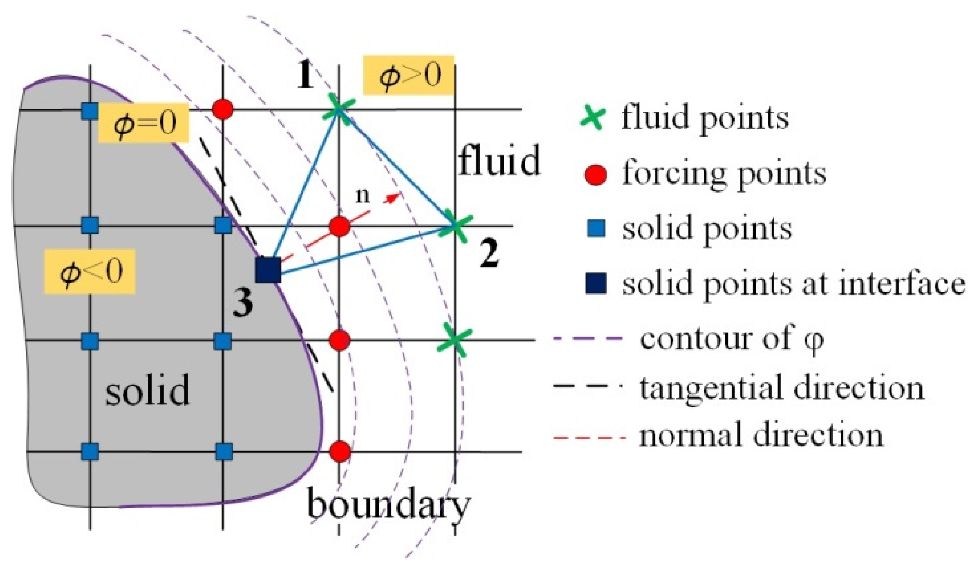
3.2. Immersed Boundary Method

For incompressible viscous flow of a Newtonian fluid with constant density and kinematic viscosity $\nu$, using tensor notation the governing equations in Cartesian coordinates can be given as:

$$\frac{\partial u_i}{\partial t}+\frac{\partial \left(u_i{u}_j\right)}{\partial x_j}=-\frac{1}{\mathsf{\rho }}\frac{\partial p}{\partial x_i}+\nu \frac{{\partial }^2{u}_i}{\partial x_j\partial x_j}+f_i$$

(15)

$$\frac{\partial u_i}{\partial x_i}=0$$

(16)

where $x_i\left(i=1,2,3\right)$ represents the Cartesian coordinates $\left(x,y,z\right)$; $u_i$ (or equivalently u, v and w) represents the velocity components in the corresponding directions; $t$ is the time; $p$ is the pressure; and $f_i$ is the external force, representing the effects of solid body on the fluid. For the laminar flow, Equations (15) and (16) are directly integrated in space and time without introducing any model. Large eddy simulation (LES) approach is used for turbulent flow, and the dynamic Samgorinsky model [23] is adopted to calculate the subgrid-scale (SGS) stress.

The staggered grid is used in our in-house developed code. The velocity components $u$, $v$, and $w$ are defined at centers of cell surfaces, and all other variables, i.e., pressure $p$ and LS function $\mathsf{\varphi }$ are defined at the center of the grid cell. The finite difference method is used for spatial discretization of the Navier–Stokes equations, and the second order Runge–Kutta (RK2) method is used for time integration. In each sub-step of the RK2 method, a fractional-step method of Kim and Moin [24] is used, and the projection method is utilized to ensure the divergence-free requirement for incompressible flow. The algorithm can be referred to Liu’s work [25]. The Krylov-based multigrid solver from the PETSc library is used to solve the pressure Poisson equation.

In Cartesian IB method, the Cartesian grid is not required to be precisely conformed to the fluid-solid interface. A forcing term $\overrightarrow{f_b}$ is introduced into the momentum equation to represent the effect of the solid body on the flow field, and it is applied on the forcing points. At first, we advance the simulation without considering the boundary effects. Then the velocity ${\overline{u}}_b$ on the forcing point is interpolated by the velocity of the surrounding fluid points (neighbouring to the forcing points on the x-grid line, y-grid line, or along the diagonal) and the solid point (the projection of forcing point). In present study, the solid points at the interface are found through the gradient operators of the LS function, and the velocities are decomposed into the tangential and normal components. As shown in Figure 4, the bilinear interpolation scheme is used to reconstruct the velocity $u_b$ at the forcing point. For the variable $\mathsf{\alpha }$ in the 2D space, the interpolation coefficients for the linear interpolation can be written as:

$$\mathsf{\alpha }=b_1+b_{2}x+b_{3}y$$

(17)

The coefficients $b_1$, $b_2$, and $b_3$ in Equation (17) can be found by solving:

$$\left[\begin{array}{c}{b}_1\\ b_2\\ b_3\end{array}\right]=A^{-1}\left[\begin{array}{c}{\mathsf{\alpha }}_1\\ {\mathsf{\alpha }}_2\\ {\mathsf{\alpha }}_3\end{array}\right]={\left[\begin{array}{ccc}1& x_1& y_1\\ 1& x_2& y_2\\ 1& x_3& y_3\end{array}\right]}^{-1}\left[\begin{array}{c}{\mathsf{\alpha }}_1\\ {\mathsf{\alpha }}_2\\ {\mathsf{\alpha }}_3\end{array}\right]$$

(18)

where $\left(x_i,y_i,z_i\right)$ with $i=1,2\mathrm{and}3$ in matrix $A$ are the point coordinates of the interpolation stencil. For the case of swimming fish, the inversion of matrix A is calculated at each time step, because of the deformed and moving fish body. After obtaining the interpolation velocity ${\overline{u}}_b$, the volume force on the forcing points is calculated as:

$$\overrightarrow{f_b}=-RH{S}^n+\frac{{\overline{u}}_b-{\overline{u}}^n}{\Delta t}$$

(19)

Here $RH{S}^n$ represents the sum of the convection term, the viscous term and the pressure gradient. The fluid force acting on the fish body can be computed by integrating all the virtual forces applied around the immersed boundary, while its direction is opposite to the momentum force [26].

3.3. Validation Cases

3.3.1. Flow Past a Sphere

The accuracy of the LS/IB method is first tested by performing the simulations of flows past a sphere. As suggested by the previous studies [27,28,29], when $Re<300$, three different laminar flow regimes exist, and they are varied with the Reynolds number. These are the steady axisymmetric flow (Re < 210), the steady nonaxisymmetric flow (210 < Re < 270), and the unsteady flow dominated by periodic vortex shedding (Re > 280). Here we simulate six cases at Re = 50, 100, 150, 200, 250 and 300, and the Reynolds number is defined on the inlet velocity $U_{\infty }$ and the sphere diameter $d$, i.e., $Re=U_{\infty }d/\nu$. Let $x$, $y$ and $z$ represent the streamwise, vertical, and spanwise directions, respectively. The computational domain in and x, y and $z$ directions is $30d\times 15d\times 15d$, and the grid number is 384 × 160 × 160. Near the sphere, the grid size is $0.02d\times 0.02d\times 0.02d$. The flow is driven by a uniform inflow with $u=U_{\infty }$ and $v=w=0$ at the left boundary of the computational domain, and a convective boundary condition is used at the outlet. Periodic conditions are imposed in both the vertical and spanwise directions.

For Re = 50, 100, 150 and 200, the flow past a sphere is steady and axisymmetric. As shown in

Table 1. Drag coefficient $C_d$ for the flow past a sphere at different Reynolds (Re) number.

Results from	Re = 50	Re = 100	Re = 150	Re = 200
Experiment [27]	1.574	1.087	0.889	0.776
Yang [28]	1.610	1.118	0.920	0.807
Johnson and Pater [29]	1.575	1.100	0.900	0.775
Present method	1.610	1.120	0.921	0.804

, the drag coefficient $C_d$ is varied with the Re number, and the results agree well with the data in references [27,28,29]. Besides, when the flow passes a sphere in streamwise direction, a steady separated bubble is formed behind the sphere. For Re = 150, the separation angle and the length of the recirculation bubble are shown in Figure 5. The topological structure is the same for other three cases, and the differences are displayed in Figure 6. At a different Re number, both the separation angle and the length of separation bubble are properly captured, and the results show good agreements with the data in references [27,28,29].

At Re = 250, the flow behind the sphere loses its axial symmetry, indicated by the nonzero lift coefficient [30]. The flow becomes unsteady at Re = 300, and the vortices are alternatively shedding behind the sphere. The drag coefficient $C_d$ and the lift coefficient $C_L$ at Re = 250 and 300 are shown in

Table 2. Force coefficients for flow past over a sphere at Re = 250.

Results from	${\mathit{C}}_{\mathit{d}}$	${\mathit{C}}_{\mathit{L}}$
Kim et al. [14]	0.701	0.059
Yang [28]	0.70	0.062
Johnson and Patel [29]	0.70	0.062
Constantinescu and Squires [31]	0.70	0.062
Present method	0.70	0.06

and

Table 3. Numerical results for flow past over a sphere at Re = 300.

Results from	${\mathit{C}}_{\mathit{d}}$	${\mathit{C}}_{\mathit{L}}$	$\mathit{S}\mathit{t}$
Kim et al. [14]	0.657	0.067	0.134
Yang [28]	0.655	0.064	0.133
Johnson and Patel [29]	0.657	0.069	0.137
Constantinescu and Squires [31]	0.655	0.065	0.136
Ploumhans et al. [32]	0.68	0.066	0.137
Present method	0.66	0.067	0.135

, respectively. At Re = 300, the Strouhal number of the shedding vortices is 0.135. All these results are in excellent agreement with the previous results [14,28,29,31], indicating that the proposed LS-IB method can capture the flow field accurately.

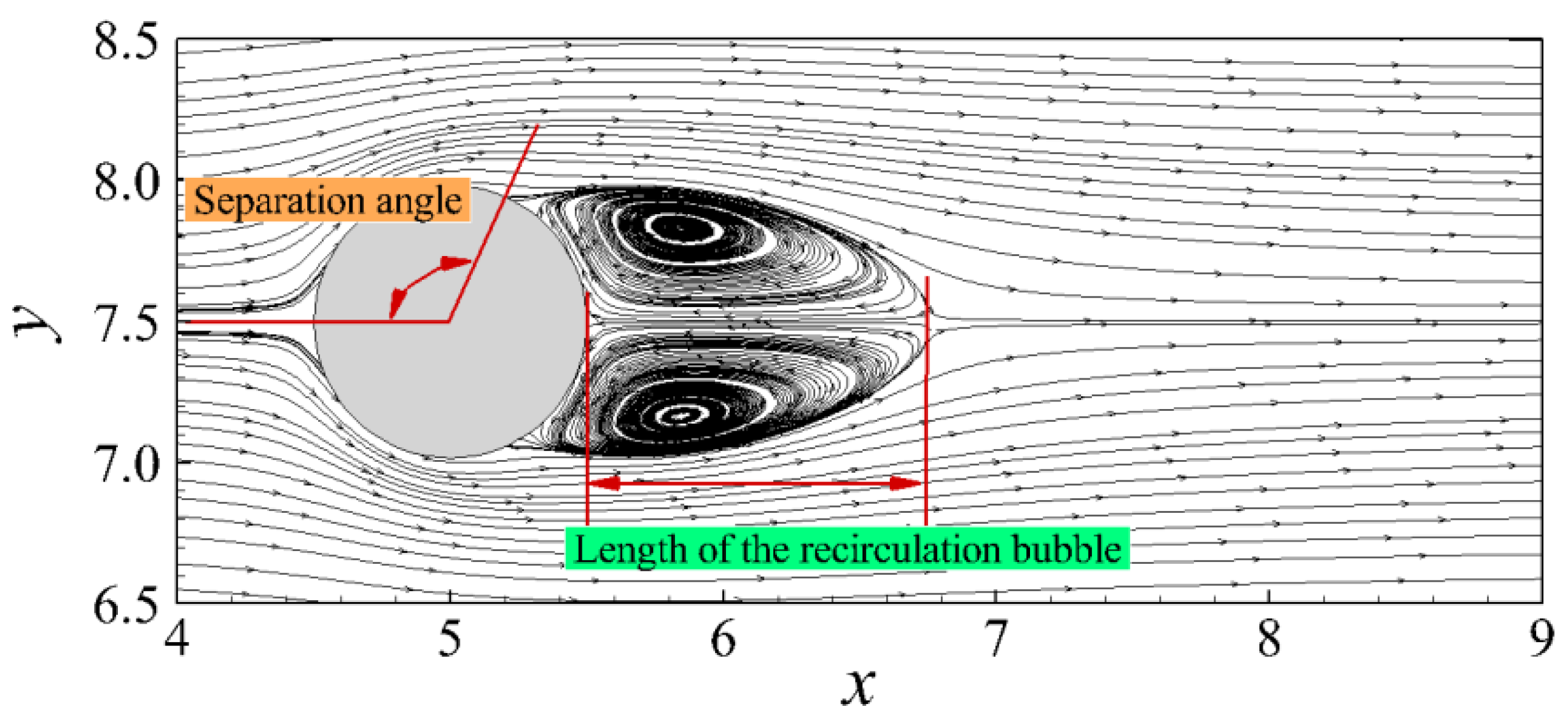
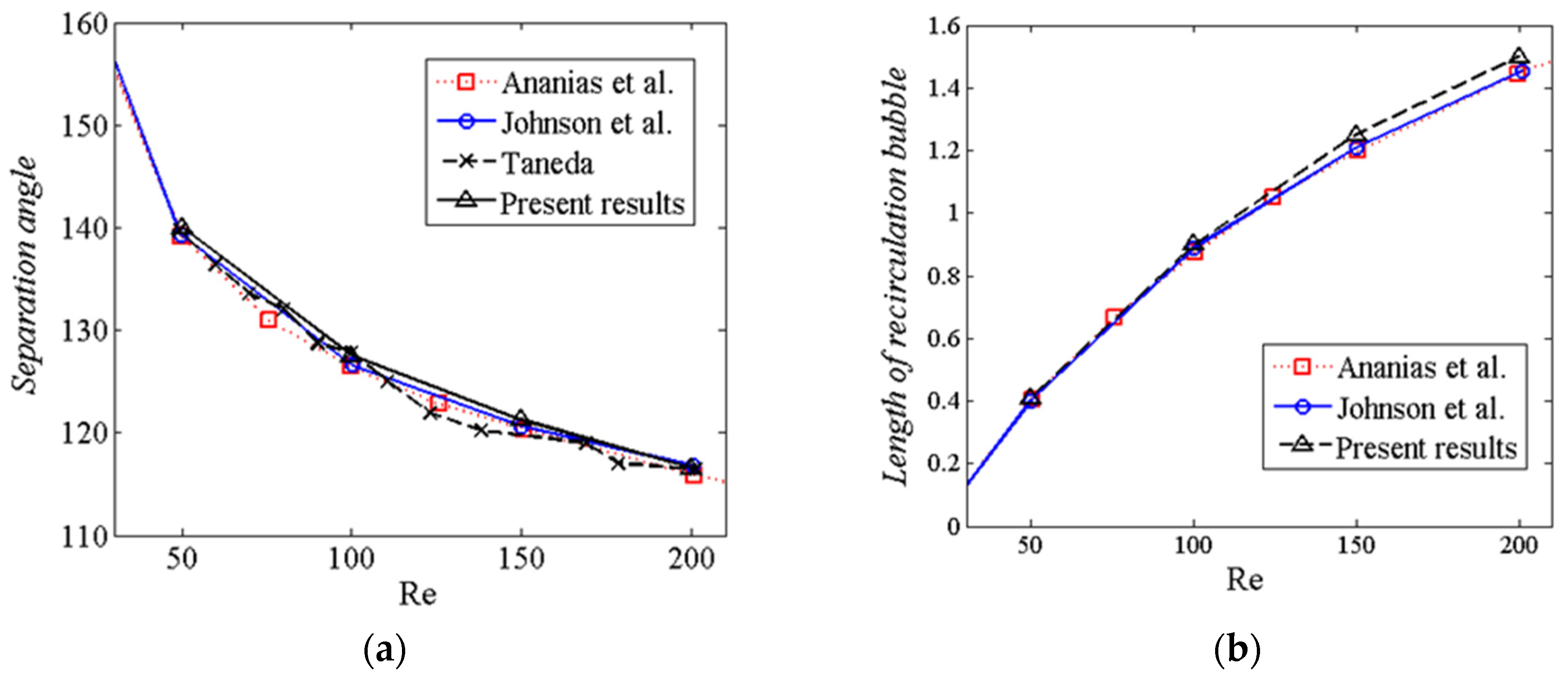
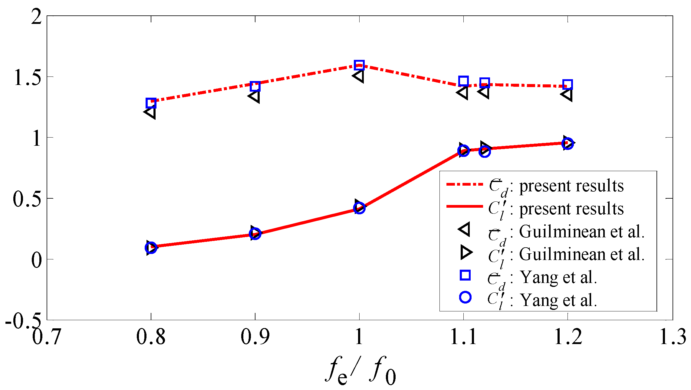
3.3.2. Flow Past a Transversely Oscillating Cylinder

To examine the capability of the method for capturing moving boundary, we further test the flow past a transversely oscillating cylinder in this section. The computational domain size in the streamwise and vertical directions is 50D × 30D, and the number of grid points is 512 × 384. D represents the diameter of the cylinder. The centre of the cylinder is 12.5D and 15D from the inlet and top boundaries, respectively. The boundary conditions are set to be the same as those for the flow past a stationary sphere. The cylinder oscillates in the vertical direction, and the Reynolds number is fixed at Re = $U_{\infty }D/\nu$ = 185. The motion of the cylinder center $\left[X_c,Y_c\right]$ is prescribed as $X_c=0$ and $Y_c\left(t\right)=Y_A\cos \left(2\mathsf{\pi }{f}_{e}t\right)$, where $Y_A=0.2D$ and $f_e$ represent the amplitude and frequency of the oscillation, respectively.

In total, we ran six cases with different normalized oscillating frequencies $f_e/f_0$: 0.8, 0.9, 1.0, 1.1, 1.12, and 1.2. Here $f_0$ denotes the frequency of vortex shedding for the flow past a stationary cylinder at Re = 185. The Strouhal number based on $f_0$ is found to be $St=f_{0}D/U_{\infty }=0.194$. The contours of the spanwise vorticity for the six cases when the cylinder reaches its extreme upper position are shown in Figure 7. Solid and dashed lines represent positive and negative vorticity, respectively. The contour interval is $0.75U_{\infty }/D$. For $f_e/f_0\le$ 1.0, the size of the attached negative vortex denoted by “A” decreases as $f_e/f_0$ increases (Figure 7a–c). At $f_e/f_0$ = 1.1, a sudden change of the vortex pattern is observed (Figure 7d). The positive attached vortex denoted by “B” becomes dominant for $f_e/f_0$ ≥ 1.1 (Figure 7d–f), and vortex A is detached. As $f_e/f_0$ increases from 1.1 to 1.2, vortex B moves upwards, and a small negative attached vortex denoted by “C” is observed. The sudden change of the vortex pattern at $f_e/f_0$ = 1.1 has been observed in literature using different numerical methods [33,34].

Figure 8 compares the mean drag coefficient ${\overline{C}}_d$ and RMS (root mean square) of the lift coefficient fluctuation $C_l^{\prime }$ with those obtained by Guilmineau et al. [33] and Yang et al. [34]. Both ${\overline{C}}_d$ and $C_l^{\prime }$ obtained in the present study agree with those given by Yang et al. [34]. Although the values of the present results of ${\overline{C}}_d$ are slightly higher than those of Guilmineau et al. [33], the differences are smaller than 3% for all test cases. The results demonstrated in Figure 8 indicate that the present algorithm can capture the moving boundary accurately.

4. Results

Based on the LS-IB method, a self-propelled model of carangiform fish with the prescribed body motion was developed, and the travelling index was varied in the range up to 50% larger or smaller than the biological value. In this study, the relation between travelling index to wave number, and its effects on swimming performance were systematically investigated.

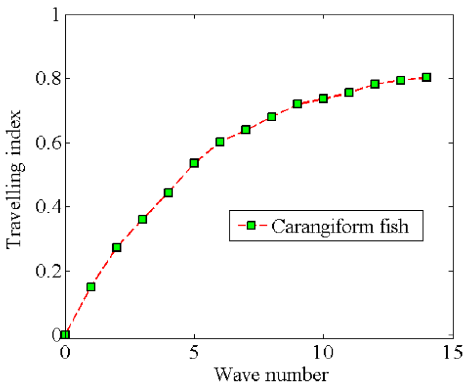
4.1. Relation between Travelling Index and Wave Number

Carangiform fish have very good integrated swimming abilities in terms of their fast speed and high efficiency. Their lateral undulations are confined to the posterior third of the body [1,2], and the mean propulsive wavelength is 98% of body length (BL; range 78%–106%) in mackerel [35]. Gray [36] also found that the propulsive wavelength is slightly greater than the body length, with the exception of the Atlantic mackerel, with a propulsive wavelength of 93% of body length. As explained, the wavelength is varied with the fish species, and this difference in present study is analysed by the COD method. As illustrated in Equation (1), the motions of carangiform fish are decomposed into the standing part and travelling part. The separated parts are shown in Figure 9, and the calculated travelling index is 0.639. This indicates that the travelling part is larger than the standing part in the midline motions. Meanwhile, it is also demonstrated that the carangiform fish prefers a swimming motion with a large component of travelling wave.

To study the relationship between wave number and travelling index, we selected the wave number as ranging from 0 to 14, while all other kinematic parameters are unchanged. The results show that the travelling index increases with the wave number until reaching a stable value, as displayed in Figure 10. Besides, if the wave number is zero, i.e., $h\left(x,t\right)=\left(a_1+a_{2}x+a_3{x}^2\right)\sin \left(\mathsf{\omega }t\right)$, this type of wave is a pure standing wave, and the travelling index is zero. For carangiform fish, the wavelength is around one body length, and it should be larger than 0.6 fish lengths, so the wave number is between 5.2 and 10.4 [1]. The range of travelling index is calculated as 0.52~0.78.

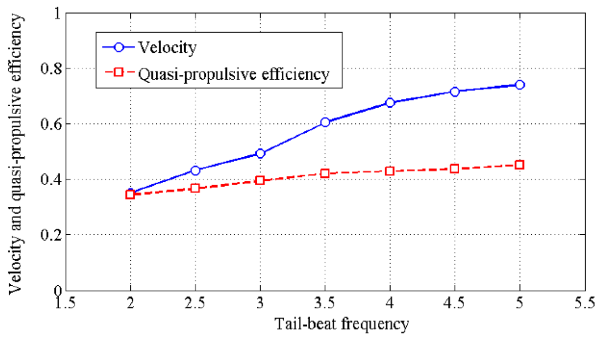
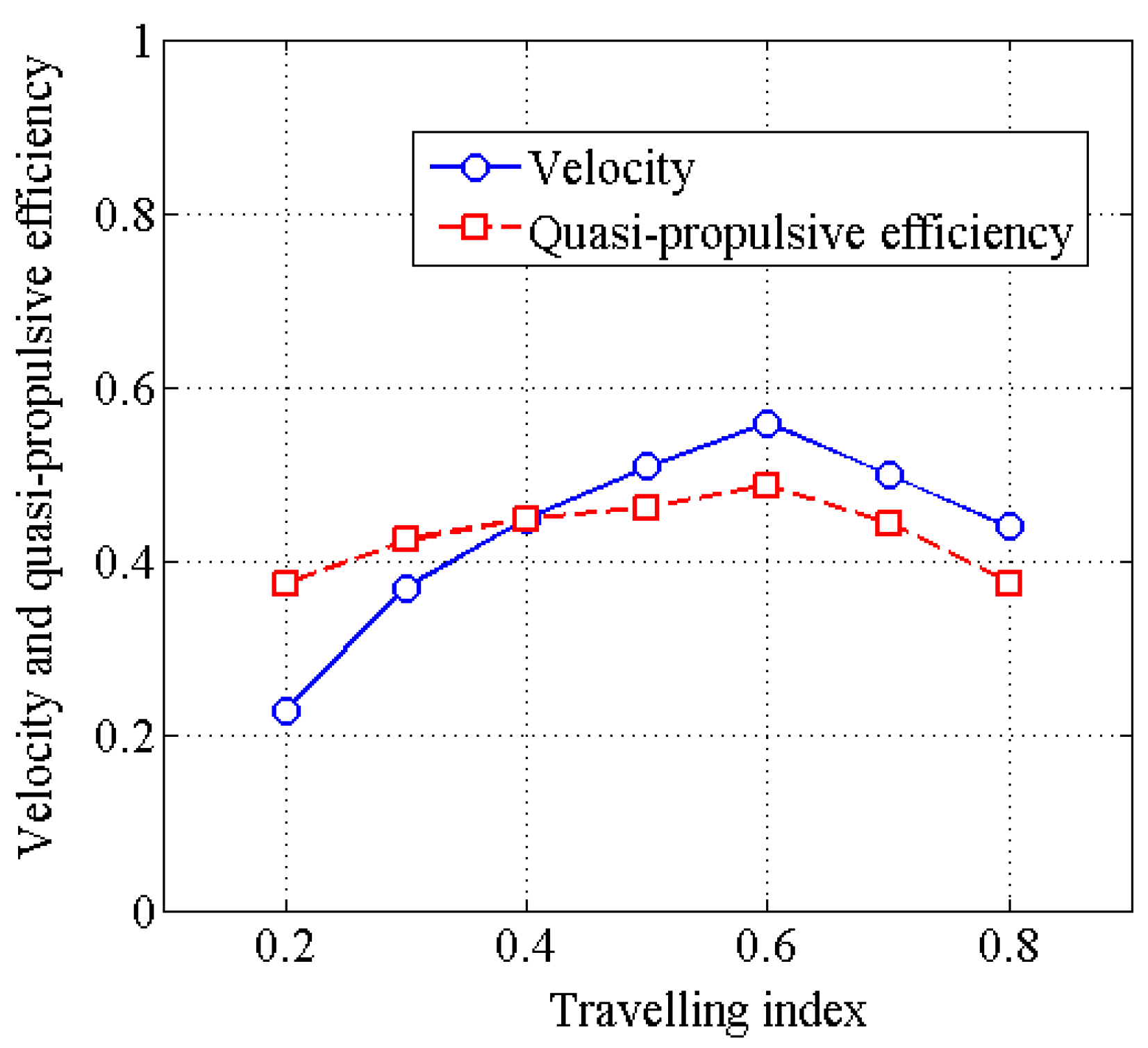
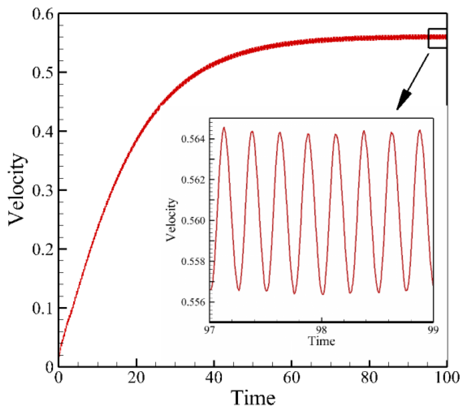
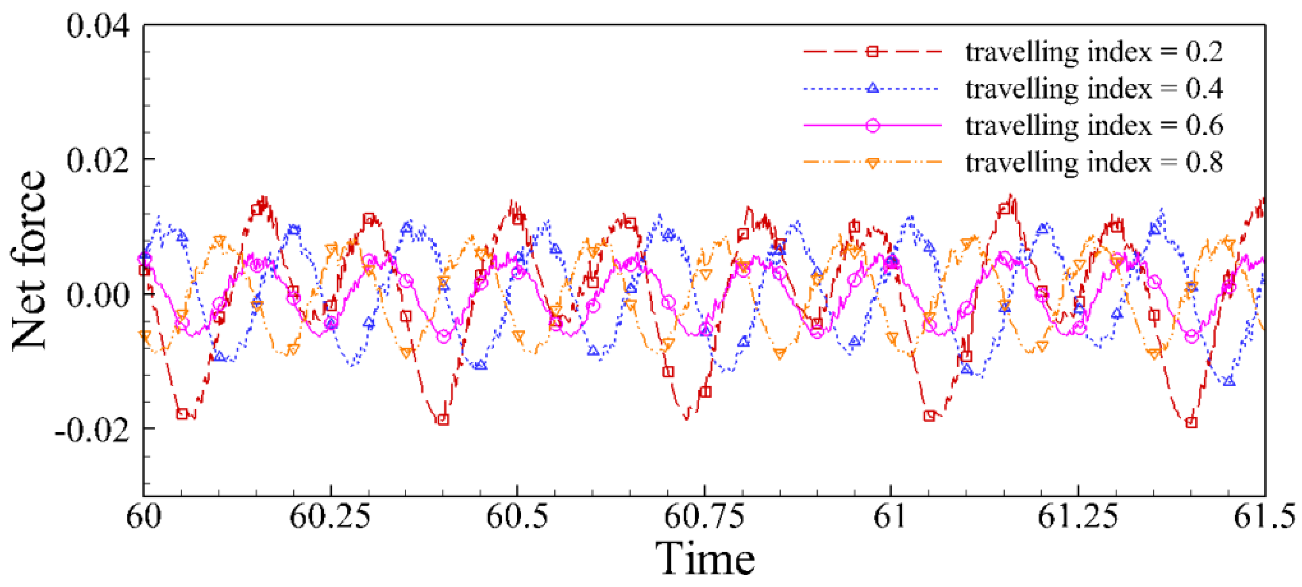
4.2. Effects of Travelling Index on Forward Speed

For carangiform fish, the travelling index of midline motions demonstrates the curvedness of fish body. To study the effects of travelling index, we varied the travelling index from 0.2 to 0.8 at the interval of 0.1, and then analysed the swimming performance though a self-propelled fish model. The relation between the forward speed and travelling index is shown in Figure 11. The results show that the forward speed is increased with the travelling index when it is less than 0.6, then it is decreased when the travelling index continually increases. As a whole, the forward speed reaches the maximum when the travelling index is around 0.6, i.e., there is an optimal range of travelling index for the carangiform fish. Besides, this result is also consistent with the biological value 0.639, and it provides a beneficial way to explain the fish-like motions of carangiform fish.

When the travelling index is 0.6, the forward speed of the virtual fish is increased until it reaches a steady state, as shown in Figure 12. It is notable that the speed at the steady state exhibits two peaks in each cycle, because of the two vortices with opposite sign shedding behind the tail. As shown in Figure 13, the reverse von Kármán vortex street is observed behind the fish tail, which is in agreement with biological observations [1,19]. The relative strength of reverse von Kármán vortices is closely related to maximizing the thrust or efficiency [37].

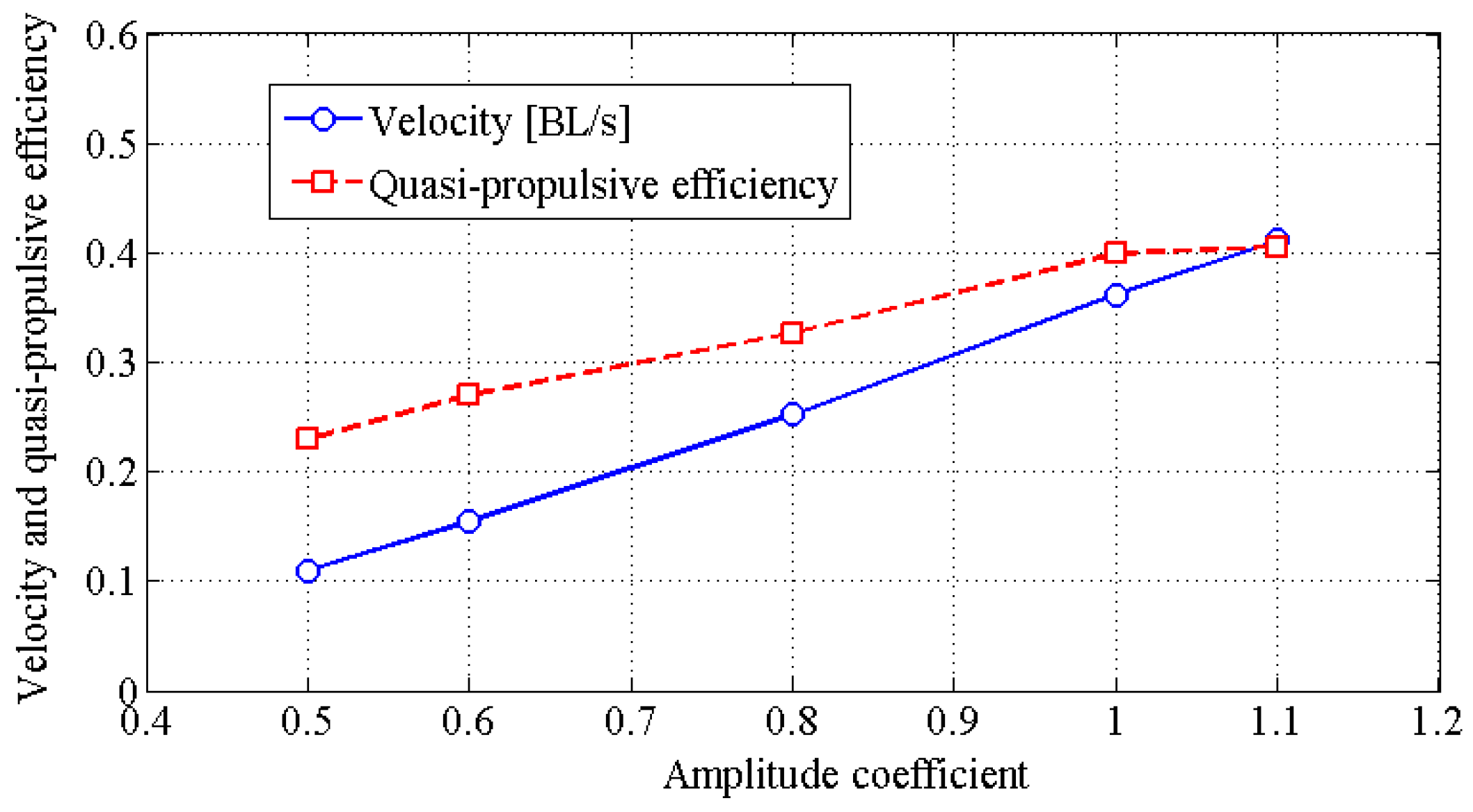
4.3. Effects of Travelling Index on Swimming Efficiency

The relation between the quasi-propulsive efficiency and the travelling index is shown in Figure 11. As expected, the quasi-propulsive efficiency reaches the maximum value when the travelling index is close to 0.6. Actually, the quasi-propulsive efficiency relied on the forward speed and the input power, rather than the net force. Therefore, it is necessary to analyse the changes of net force around the fish body. At the steady state, the thrust and drag forces are balanced, i.e., the mean net force is zero. In Figure 14, the thrust is decreased with travelling index when the travelling index is smaller than 0.6. Similarly, the net force with small oscillations also exhibits two peaks in each tail-beat cycle. As a whole, when the travelling index is close to the optimal range, both the forward speed and the quasi-propulsive efficiency of carangiform fish reach the maximum values. In a manner similar to the flow past a wavy wall, however, the thrust of carangiform fish is reduced to the minimum due to the flow separation and the distribution of pressure [38,39,40].

Combined with Figure 11 and Figure 14, these results provide an explanation for the biological feat as to why the carangiform fish adjust the travelling index to achieve their fast and efficient propulsive performance. As discussed, the vorticity fields and the pressure distribution are changed dramatically if the midline motions are changed. The vortices of the fish model with fast speed are stronger than those with slow speed, which modifies the distribution of the pressure, and thus changes the force characteristics and power consumption. This study can be taken as an explanation of the observation that fish change their waveform to propel themselves faster or more efficiently.

5. Discussion

In general, the fish-like motions are often described by other two parameters: the tail-beat frequency and the amplitude envelope. To compare the relative effects of the travelling index, we also investigated the influences of tail-beat frequency and amplitude envelope on swimming performance. The tail-beat frequency was increased from 2.0 Hz to 5.0 Hz at the interval of 0.5 Hz, and other kinematic parameters were the same as the values in Section 2. As shown in Figure 15, both the forward speed and the quasi-propulsive efficiency increase with the tail-beat frequency. As a whole, when the fish increases tail-beat frequency, the forward speed is increased significantly, but the swimming efficiency is increased only slightly. These results are consistent with biological observations [41].

On the other hand, we changed the amplitude by timing an amplitude coefficient $C$, i.e., A(x) = C(a₁ + a₂x + a₃x²) , and the amplitude coefficient was selected as 0.5, 0.6, 0.8, 1.0 and 1.1. The relationships among the amplitude, the forward speed and the quasi-propulsive efficiency are presented in Figure 16. With the incensement of amplitude, both the forward speed and the quasi-propulsive efficiency are significantly increased, especially when the amplitude coefficient is less than one. This results suggest that for designing a robotic fish, a large amplitude is required to obtain the desired swimming performance.

Combined with the numerical results in Figure 11, Figure 15 and Figure 16, we found that although the tail-beat frequency and amplitude contribute to improve the propulsive abilities, they are often somewhat limited. For example, swimming fish always maintain their large amplitude (0.2 BL) during steady locomotion [41]. In contrast however, the travelling index has an optimal range for optimizing swimming performance with the maximum speed and efficiency, which is consistent with the biological studies and observations [1,18].

6. Conclusions

To understand the effects of waveform on swimming performance, a self-propelled model of carangiform fish was developed by the modified LS-IB method. In this study, the midline motions of fish body were decomposed by the COD method, and the travelling index was used to study the waveform of fish-like movements. The morphological and kinematics data of the fish model were introduced from true fish, and the net force, the forward speed and the quasi-propulsive efficiency have been used to evaluate the swimming performance. Our results show that for carangiform fish, there is an optimal range of travelling index to obtain maximum forward speed and the highest swimming efficiency. Therefore, we predict that for swimming fish, there is an optimal range of travelling index for optimizing their integrative swimming performance. By comparison, we found that the forward speed mainly relies on the travelling index and tail-beat frequency, while the swimming efficiency is increased with the tail-beat frequency and amplitude coefficient. It is probable that the swimming abilities of carangiform fish could be further improved by adjusting the travelling index, the amplitude and the tail-beat frequency in parallel. The results presented in this work provide a guideline for future studies in this area.

References

1. Sfakiotakis, M.; Lane, D.M.; Davies, J.B.C. Review of fish swimming modes for aquatic locomotion. IEEE J. Ocean. Eng. 1999, 24, 237–252. [Google Scholar] [CrossRef]
2. Videler, J.J. Fish Swimming; Chapman and Hall: London, UK, 1993. [Google Scholar]
3. Barrett, D.S.; Triantafyllou, M.S.; Yue, D.K.P. Drag reduction in fish-like locomotion. J. Fluid Mech. 1999, 392, 183–212. [Google Scholar] [CrossRef]
4. Lighthill, M.J. Large-amplitude elongated-body theory of fish locomotion. Proc. R. Soc. Lond. B 1971, 179, 125–138. [Google Scholar] [CrossRef]
5. Anderson, E.J.; McGillis, W.R.; Grosenbaugh, M.A. The boundary layer of swimming fish. J. Exp. Biol. 2001, 201, 81–102. [Google Scholar]
6. Feeny, B.F. A complex orthogonal decomposition for wave motion analysis. J. Sound Vib. 2008, 310, 77–90. [Google Scholar] [CrossRef]
7. Feeny, B.F.; Feeny, A.K. Complex modal analysis of the swimming motion of a whiting. J. Vib. Acoust. 2013, 135, 021004. [Google Scholar] [CrossRef]
8. Carling, J.; Williams, T.L.; Bowtell, G. Self-propelled anguilliform swimming: Simultaneous solution of the two-dimensional Navier-Stokes equations and Newton's laws of motion. J. Exp. Biol. 1998, 201, 3143–3166. [Google Scholar] [PubMed]
9. Borazjani, I.; Sotiropoulos, F. On the role of form and kinematics on the hydrodynamics of self-propelled body/caudal fin swimming. J. Exp. Biol. 2010, 213, 89–107. [Google Scholar] [CrossRef] [PubMed]
10. Tian, F.B.; Xu, Y.Q.; Tang, X.Y.; Deng, Y.L. Study on a self-propelled fish swimming in viscous fluid by a finite element method. J. Mech. Med. Biol. 2013, 13, 1340012. [Google Scholar] [CrossRef]
11. Tian, F.B.; Dai, H.; Luo, H.; Doyle, J.F.; Rousseau, B. Fluid-structure interaction involving large deformations: 3D simulations and applications to biological systems. J. Comput. Phys. 2014, 258, 451–469. [Google Scholar] [CrossRef] [PubMed]
12. Mittal, R.; Dong, H.; Bozkurttas, M.; Najjar, F.M.; Vargas, A.; von Loebbecke, A. A versatile sharp interface immersed boundary method for incompressible flows with complex boundaries. J. Comput. Phys. 2008, 227, 4825–4852. [Google Scholar] [CrossRef] [PubMed]
13. Luo, H.; Dai, H.; Ferreira de Sousa, P.; Yin, B. On numerical oscillation of the direct-forcing immersed-boundary method for moving boundaries. Comput. Fluids 2012, 56, 61–76. [Google Scholar] [CrossRef]
14. Kim, J.; Kim, D.; Choi, H. An immersed boundary finite volume method for simulations of flow in complex geometries. J. Comput. Phys. 2001, 171, 132–150. [Google Scholar] [CrossRef]
15. Cheny, Y.; Botella, O. The LS-STAG method: A new immersed boundary/level-set method for the computation of incompressible viscous flows in complex moving geometries with good conservation properties. J. Comput. Phys. 2010, 229, 1043–1076. [Google Scholar] [CrossRef]
16. Meyer, M.; Devesa, A.; Hickel, S.; Hu, X.; Adams, N. A conservative immersed interface method for Large-Eddy Simulation of incompressible flows. J. Comput. Phys. 2010, 229, 6300–6317. [Google Scholar] [CrossRef]
17. Shrivastava, M.; Agrawal, A.; Sharma, A. A novel level set-based immersed-boundary method for CFD simulation of moving-boundary problems. Numer. Heat. Transf. B 2013, 63, 304–326. [Google Scholar] [CrossRef]
18. Alvarado, P.V.Y. Design of Biomimetic Compliant Devices for Locomotion in Liquid Environments; Massachusetts Institute of Technology: Cambridge, MA, USA, 2007. [Google Scholar]
19. Taylor, G.K.; Nudds, R.L.; Thomas, A.L.R. Flying and swimming animals cruise at a Strouhal number tuned for high power efficiency. Nature 2003, 425, 707–711. [Google Scholar] [CrossRef] [PubMed]
20. Maertens, A.P.; Triantafyllou, M.S.; Yue, D.K.P. Efficiency of fish propulsion. Bioinspir. Biomim. 2015, 10, 46013–46023. [Google Scholar] [CrossRef] [PubMed]
21. Osher, S.; Sethian, J.A. Fronts propagating with curvature dependent speed: Algorithms based on Hamilton–Jacobi formulations. J. Comput. Phys. 1988, 79, 12–49. [Google Scholar] [CrossRef]
22. Sethian, J.A. Level Set Methods and Fast Marching Methods; Cambridge University Press: Cambridge, UK, 1999. [Google Scholar]
23. Germano, M.; Piomelli, U.; Moin, P.; Cabot, W.H. A dynamic subgrid-scale eddy viscosity model. Phys. Fluids 1991, 3, 1760–1765. [Google Scholar] [CrossRef]
24. Kim, J.; Moin, P. Application of a fractional-step method to incompressible Navier-Stokes equations. J. Comput. Phys. 1985, 59, 308–323. [Google Scholar] [CrossRef]
25. Liu, Y. Numerical Study of Strong Free Surface Flow and Breaking Waves; The Johns Hopkins University: Baltimore, MD, USA, 2013. [Google Scholar]
26. Le, D.V.; Khoo, B.C.; Peraire, J. An immersed interface method for viscous incompressible flows involving rigid and flexible boundaries. J. Comput. Phys. 2006, 220, 109–138. [Google Scholar] [CrossRef]
27. Clift, R.; Grace, J.R.; Weber, M.E. Bubbles, Drops, and Particles; Courier Corporation: North Chelmsford, MA, USA, 2005. [Google Scholar]
28. Yang, J.M. An Embedded Boundary Formulation for Large-Eddy Simulation of Turbulent Flows Interacting with Moving Boundaries; University of Maryland: Baltimore, MD, USA, 2005. [Google Scholar]
29. Johnson, T.A.; Patel, V.C. Flow past a sphere up to a Reynolds number of 300. J. Fluid Mech. 1999, 378, 19–70. [Google Scholar] [CrossRef]
30. Tomboulides, A.G.; Orszag, S.A. Numerical investigation of transitional and weak turbulent flow past a sphere. J. Fluid Mech. 2000, 416, 45–73. [Google Scholar] [CrossRef]
31. Constantinescu, G.S.; Squires, K.D. LES and DES investigations of turbulent flow over a sphere. AIAA Pap. 2000, 2000–0540. [Google Scholar] [CrossRef]
32. Ploumhans, P.; Winckelmans, G.S.; Salmon, J.K.; Leonard, A.; Warren, M.S. Vortex methods for direct numerical simulation of three-dimensional bluff body flows: Applications to the sphere at Re = 300, 500 and 1000. J. Comput. Phys. 2002, 178, 427–463. [Google Scholar] [CrossRef]
33. Guilmineau, E.; Queutey, P. A numerical simulation of vortex shedding from an oscillating circular cylinder. J. Fluid Struct. 2002, 16, 773–794. [Google Scholar] [CrossRef]
34. Yang, J.; Balaras, E. An embedded-boundary formulation for large-eddy simulation of turbulent flows interacting with moving boundaries. J. Comput. Phys. 2006, 215, 12–40. [Google Scholar] [CrossRef]
35. Videler, J.J.; Hess, F. Fast continuous swimming of two pelagic predators, saithe (Pollachius virens) and mackerel (Scomber scombrus)—A kinematic analysis. J. Exp. Biol. 1984, 109, 209–228. [Google Scholar]
36. Gray, J. Studies in animal locomotion III: The propulsive mechanism of the whiting (Gadus merlangus). J. Exp. Biol. 1933, 10, 391–402. [Google Scholar]
37. Müller, U.K.; Smit, J.; Stamhuis, E.J.; Videler, J.J. How the body contributes to the wave in undulatory fish swimming. J. Exp. Biol. 2001, 204, 2751–2762. [Google Scholar] [PubMed]
38. Shen, L.; Zhang, X.; Yue, D.K.P.; Triantafyllou, M.S. Turbulent flow over a flexible wall undergoing a streamwise travelling wave motion. J. Fluid Mech. 2003, 484, 197–221. [Google Scholar] [CrossRef]
39. Tian, F.B.; Lu, X.Y.; Luo, H. Propulsive performance of a body with a traveling wave surface. Phys. Rev. E 2012, 86, 016304. [Google Scholar] [CrossRef] [PubMed]
40. Liu, G.; Yu, Y.L.; Tong, B.G. Flow control by means of a traveling curvature wave in fishlike escape responses. Phys. Rev. E 2011, 84, 056312. [Google Scholar] [CrossRef] [PubMed]
41. Bainbridge, R. The speed of swimming of fish as related to size and to the frequency and amplitude of the tail beat. J. Exp. Biol. 1958, 35, 109–133. [Google Scholar]
Figure 1. Illustration of kinematics variables used to describe the swimming fish. L : full length of fish body; R(x): half-height; r(x): half-width.
Applsci 07 00149 g001
Figure 2. The midline motions of carangiform fish during one tail-beat period.
Applsci 07 00149 g002
Figure 3. The value of the level set (LS) function ϕ : (a) before the re-initialization process; (b) after the re-initialization process.
Applsci 07 00149 g003
Figure 4. Sketch of the level-set/immersed boundary method.
Applsci 07 00149 g004
Figure 5. Axisymmetric streamlines past the sphere at Re = 150.
Applsci 07 00149 g005
Figure 6. Wake structure versus Reynolds number: (a) separation angle; (b) bubble length.
Applsci 07 00149 g006
Figure 7. Contours of instantaneous spanwise vorticity when the oscillating cylinder reaches its extreme upper position for (a) f e / f 0 = 0.8; (b) f e / f 0 = 0.9; (c) f e / f 0 = 1.0; (d) f e / f 0 = 1.1; (e) f e / f 0 = 1.12; and (f) f e / f 0 = 1.2.
Applsci 07 00149 g007
Figure 8. Mean drag coefficient C ¯ d and RMS of lift coefficient C l for flow past a transversely oscillating cylinder at different f e / f 0 .
Applsci 07 00149 g008
Figure 9. The separated standing and travelling parts of the midline motion of the carangiform fish. (a) standing part; (b) travelling part.
Applsci 07 00149 g009
Figure 10. The changing pattern of travelling index along with the wave number.
Applsci 07 00149 g010
Figure 11. Effects of travelling index on the swimming performance of carangiform fish.
Applsci 07 00149 g011
Figure 12. Time history of the forward velocity of the swimming carangiform fish.
Applsci 07 00149 g012
Figure 13. Reverse von Kármán vortex street behind the tail of swimming carangiform fish (solid and dashed lines represent positive and negative values of vorticity, respectively).
Applsci 07 00149 g013
Figure 14. Time history of the net force of carangiform fish at different travelling indices.
Applsci 07 00149 g014
Figure 15. Effects of tail-beat frequency on the swimming performance of carangiform fish.
Applsci 07 00149 g015
Figure 16. Effects of amplitude coefficient on the swimming performance of carangiform fish.
Applsci 07 00149 g016