Fusion of Linear and Mel Frequency Cepstral Coefficients for Automatic Classification of Reptiles


Abstract
:1. Introduction
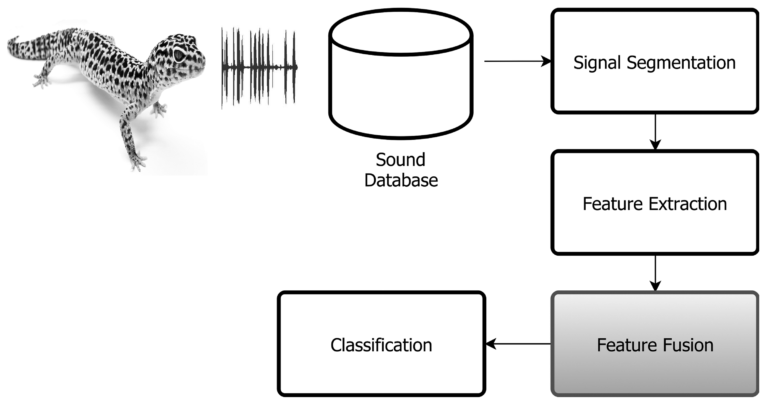
2. Proposed Method
2.1. Segmentation
- Find and such that , placing the nth syllable in . The amplitude of this point is calculated as Equation (1):
- If , the segmentation process is stopped, as the signal amplitude is inferior to the stopping criteria β. For reptile sounds, β has been set to 25 dB.
- From , seek the highest peak of for and , until for both sides. Thus, the starting and ending times of the nth syllable are denoted as, and .
- Save the amplitude trajectories as the nth syllable.
- Delete the nth syllable from the matrix and set .
- Repeat from Step 1 until the end of the spectrogram.
2.2. Feature Extraction
3. Classification System
3.1. K-Nearest Neighbor
3.2. Support Vector Machine
4. Experimental Procedure
4.1. Sound Dataset
4.2. Results and Discussion
5. Conclusions and Future Work
Author Contributions
Conflicts of Interest
References
- Gans, C.; Maderson, P.F. Sound producing mechanisms in recent reptiles: Review and comment. Am. Zool. 1973, 13, 1195–1203. [Google Scholar] [CrossRef]
- Bauer, A.M. Geckos: The Animal Answer Guide; JHU Press: Baltimore, MD, USA, 2013. [Google Scholar]
- Galeotti, P.; Sacchi, R.; Fasola, M.; Ballasina, D. Do mounting vocalisations in tortoises have a communication function? A comparative analysis. Herpetol. J. 2005, 15, 61–71. [Google Scholar]
- Vergne, A.; Pritz, M.; Mathevon, N. Acoustic communication in crocodilians: From behaviour to brain. Biol. Rev. 2009, 84, 391–411. [Google Scholar] [CrossRef] [PubMed]
- Giles, J.C.; Davis, J.A.; McCauley, R.D.; Kuchling, G. Voice of the turtle: The underwater acoustic repertoire of the long-necked freshwater turtle, Chelodina oblonga. J. Acoust. Soc. Am. 2009, 126, 434–443. [Google Scholar] [CrossRef] [PubMed]
- Labra, A.; Silva, G.; Norambuena, F.; Velásquez, N.; Penna, M. Acoustic features of the weeping lizard’s distress call. Copeia 2013, 2013, 206–212. [Google Scholar] [CrossRef]
- Bell, T.P. A novel technique for monitoring highly cryptic lizard species in forests. Herpetol. Conserv. Biol. 2009, 4, 415–425. [Google Scholar]
- Blumstein, D.T.; Mennill, D.J.; Clemins, P.; Girod, L.; Yao, K.; Patricelli, G.; Deppe, J.L.; Krakauer, A.H.; Clark, C.; Cortopassi, K.A.; et al. Acoustic monitoring in terrestrial environments using microphone arrays: Applications, technological considerations and prospectus. J. Appl. Ecol. 2011, 48, 758–767. [Google Scholar] [CrossRef]
- Fitzpatrick, M.C.; Preisser, E.L.; Ellison, A.M.; Elkinton, J.S. Observer bias and the detection of low-density populations. Ecol. Appl. 2009, 19, 1673–1679. [Google Scholar] [CrossRef] [PubMed]
- Fuchida, M.; Pathmakumar, T.; Mohan, R.E.; Tan, N.; Nakamura, A. Vision-Based Perception and Classification of Mosquitoes Using Support Vector Machine. Appl. Sci. 2017, 7, 51. [Google Scholar] [CrossRef]
- Zhao, M.; Li, Z.; He, W. Classifying Four Carbon Fiber Fabrics via Machine Learning: A Comparative Study Using ANNs and SVM. Appl. Sci. 2016, 6, 209. [Google Scholar] [CrossRef]
- Li, H.; Yuan, D.; Wang, Y.; Cui, D.; Cao, L. Arrhythmia Classification Based on Multi-Domain Feature Extraction for an ECG Recognition System. Sensors 2016, 16, 1744. [Google Scholar] [CrossRef] [PubMed]
- Acevedo, M.A.; Corrada-Bravo, C.J.; Corrada-Bravo, H.; Villanueva-Rivera, L.J.; Aide, T.M. Automated classification of bird and amphibian calls using machine learning: A comparison of methods. Ecol. Inform. 2009, 4, 206–214. [Google Scholar] [CrossRef]
- Brandes, T.S. Feature vector selection and use with hidden Markov models to identify frequency-modulated bioacoustic signals amidst noise. IEEE Trans. Audio Speech 2008, 16, 1173–1180. [Google Scholar] [CrossRef]
- Zhu, L.-Q. Insect sound recognition based on mfcc and pnn. In Proceedings of the 2011 International Conference on Multimedia and Signal Processing (CMSP), Guilin, China, 14–15 May 2011; Volume 2, pp. 42–46.
- Henríquez, A.; Alonso, J.B.; Travieso, C.M.; Rodríguez-Herrera, B.; Bolaños, F.; Alpízar, P.; López-de Ipina, K.; Henríquez, P. An automatic acoustic bat identification system based on the audible spectrum. Expert Syst. Appl. 2014, 41, 5451–5465. [Google Scholar] [CrossRef]
- Zhou, X.; Garcia-Romero, D.; Duraiswami, R.; Espy-Wilson, C.; Shamma, S. Linear versus mel frequency cepstral coefficients for speaker recognition. In Proceedings of the 2011 IEEE Workshop on Automatic Speech Recognition and Understanding (ASRU), Waikoloa, HI, USA, 11–15 December 2011; pp. 559–564.
- Cover, T.M.; Hart, P.E. Nearest neighbor pattern classification. IEEE Trans. Inf. Theory 1967, 13, 21–27. [Google Scholar] [CrossRef]
- Burges, C.J. A tutorial on support vector machines for pattern recognition. Data Min. Knowl. Discov. 1998, 2, 121–167. [Google Scholar] [CrossRef]
- Härmä, A. Automatic identification of bird species based on sinusoidal modeling of syllables. In Proceedings of the 2003 IEEE International Conference on Acoustics, Speech, and Signal Processing, Hong Kong, China, 6–10 April 2003; Volume 5, p. V-545.
- Tiwari, V. MFCC and its applications in speaker recognition. Int. J. Emerg. Technol. 2010, 1, 19–22. [Google Scholar]
- Yuan, C.L.T.; Ramli, D.A. Frog sound identification system for frog species recognition. In Context-Aware Systems and Applications; Springer: Berlin, Germany, 2013; pp. 41–50. [Google Scholar]
- Jaafar, H.; Ramli, D.A.; Rosdi, B.A.; Shahrudin, S. Frog identification system based on local means k-nearest neighbors with fuzzy distance weighting. In The 8th International Conference on Robotic, Vision, Signal Processing & Power Applications; Springer: Berlin, Germany, 2014; pp. 153–159. [Google Scholar]
- Xie, J.; Towsey, M.; Truskinger, A.; Eichinski, P.; Zhang, J.; Roe, P. Acoustic classification of Australian anurans using syllable features. In Proceedings of the 2015 IEEE Tenth International Conference on Intelligent Sensors, Sensor Networks and Information Processing (ISSNIP), Singapore, 7–9 April 2015; pp. 1–6.
- Ganchev, T.; Potamitis, I.; Fakotakis, N. Acoustic monitoring of singing insects. In Proceedings of the IEEE International Conference on Acoustics, Speech and Signal Processing, ICASSP 2007, Honolulu, HI, USA, 16–20 April 2007; Volume 4, p. IV-721.
- Fagerlund, S. Bird species recognition using support vector machines. EURASIP J. Appl. Signal Proc. 2007, 2007, 64. [Google Scholar] [CrossRef]
- Hsu, C.W.; Lin, C.J. A comparison of methods for multiclass support vector machines. IEEE Trans. Neural Netw. 2002, 13, 415–425. [Google Scholar] [PubMed]
- Powers, D.M. Evaluation: From Precision, Recall and F-measure to ROC, Informedness, Markedness and Correlation; Bioinfo Publications: Pune, India, 2011. [Google Scholar]
- Chang, C.C.; Lin, C.J. LIBSVM: A library for support vector machines. ACM Trans. Intell. Syst. Technol. (TIST) 2011, 2, 27. [Google Scholar] [CrossRef]
- Boser, B.E.; Guyon, I.M.; Vapnik, V.N. A training algorithm for optimal margin classifiers. In Proceedings of the Fifth Annual Workshop on Computational Learning Theory, Pittsburgh, PA, USA, 27–29 July 1992; pp. 144–152.
- The Animal Sound Archive. Berlin Natural Museum. Available online: http://www.tierstimmenarchiv.de (accessed on 26 July 2015).
- California Reptiles and Amphibians. Available online: http://www.californiaherps.com (accessed on 26 July 2015).
- California Turtle and Tortoise Club. Available online: http://www.tortoise.org (accessed on 23 July 2015).

| No. | Scientific Name | Family | Number of Syllables (Ns) | No. | Scientific Name | Family | Number of Syllables (Ns) |
|---|---|---|---|---|---|---|---|
| 1 | Crotalus lepidus | Squamata | 12 | 2 | Crotalus molossus | Squamata | 33 |
| 3 | Crotalus oreganus helleri | Squamata | 34 | 4 | Crotalus tigris | Squamata | 22 |
| 5 | Crotalus willardi | Squamata | 5 | 6 | Crotalus atrox | Squamata | 6 |
| 7 | Crotalus scutulatus | Squamata | 64 | 8 | Crotalus oreganus oreganus | Squamata | 18 |
| 9 | Caiman crocodilus | Crocodilia | 5 | 10 | Chelonoidis nigra | Testudines | 6 |
| 11 | Crotalus molossus | Squamata | 10 | 12 | Centrochelys sulcata | Testudines | 29 |
| 13 | Testudo horsfieldii | Testudines | 20 | 14 | Gekko gecko | Gekkonidae | 16 |
| 15 | Alligator sinensis | Crocodilia | 18 | 16 | Alligator mississippiensis | Crocodilia | 5 |
| 17 | Crotalus durissus | Squamata | 51 | 18 | Crotalus horridus | Squamata | 53 |
| 19 | Kinixys belliana | Testudines | 13 | 20 | Geochelone chilensis | Testudines | 14 |
| 21 | Testudo kleinmanni | Testudines | 95 | 22 | Geochelone carbonaria | Testudines | 17 |
| 23 | Geochelone denticulata | Testudines | 115 | 24 | Crotalus cerastes | Squamata | 642 |
| 25 | Heloderma suspectum | Squamata | 383 | 26 | Hemidactylus turcicu | Squamata | 199 |
| 27 | Ophiophagus hannah | Squamata | 10 |
| No. | kNN | SVM | ||||
|---|---|---|---|---|---|---|
| MFCC | LFCC | MFCC/LFCC | MFCC | LFCC | MFCC/LFCC | |
| 1 | 98.67% ± 0.11 | 97.00% ± 0.17 | 98.67% ± 0.11 | 99.67% ± 0.06 | 96.00% ± 0.20 | 98.33% ± 0.13 |
| 2 | 100.00% ± 0.00 | 100.00% ± 0.00 | 100.00% ± 0.00 | 100.00% ± 0.00 | 100.00% ± 0.00 | 100.00% ± 0.00 |
| 3 | 99.53% ± 0.07 | 96.82% ± 0.18 | 97.65% ± 0.15 | 99.41% ± 0.08 | 99.06% ± 0.10 | 99.65% ± 0.06 |
| 4 | 98.00% ± 0.14 | 98.55% ± 0.12 | 96.00% ± 0.20 | 100.00% ± 0.00 | 97.09% ± 0.17 | 99.45% ± 0.07 |
| 5 | 100.00% ± 0.00 | 78.00% ± 0.42 | 97.00% ± 0.17 | 100.00% ± 0.00 | 90.00% ± 0.30 | 99.00% ± 0.10 |
| 6 | 100.00% ± 0.00 | 100.00% ± 0.00 | 100.00% ± 0.00 | 100.00% ± 0.00 | 100.00% ± 0.00 | 100.00% ± 0.00 |
| 7 | 97.88% ± 0.14 | 94.25% ± 0.23 | 95.31% ± 0.21 | 88.31% ± 0.32 | 96.63% ± 0.18 | 98.81% ± 0.11 |
| 8 | 100.00% ± 0.00 | 100.00% ± 0.00 | 100.00% ± 0.00 | 100.00% ± 0.00 | 99.33% ± 0.08 | 100.00% ± 0.00 |
| 9 | 100.00% ± 0.00 | 100.00% ± 0.00 | 100.00% ± 0.00 | 100.00% ± 0.00 | 100.00% ± 0.00 | 100.00% ± 0.00 |
| 10 | 100.00% ± 0.00 | 100.00% ± 0.00 | 100.00% ± 0.00 | 100.00% ± 0.00 | 100.00% ± 0.00 | 100.00% ± 0.00 |
| 11 | 100.00% ± 0.00 | 100.00% ± 0.00 | 100.00% ± 0.00 | 100.00% ± 0.00 | 100.00% ± 0.00 | 100.00% ± 0.00 |
| 12 | 100.00% ± 0.00 | 100.00% ± 0.00 | 100.00% ± 0.00 | 100.00% ± 0.00 | 100.00% ± 0.00 | 100.00% ± 0.00 |
| 13 | 98.80% ± 0.11 | 95.60% ± 0.21 | 99.80% ± 0.04 | 98.40% ± 0.13 | 98.80% ± 0.11 | 100.00% ± 0.00 |
| 14 | 100.00% ± 0.00 | 100.00% ± 0.00 | 100.00% ± 0.00 | 100.00% ± 0.00 | 100.00% ± 0.00 | 100.00% ± 0.00 |
| 15 | 78.22% ± 0.41 | 79.11% ± 0.41 | 87.78% ± 0.33 | 67.56% ± 0.47 | 78.67% ± 0.41 | 86.22% ± 0.35 |
| 16 | 100.00% ± 0.00 | 100.00% ± 0.00 | 100.00% ± 0.00 | 80.00% ± 0.40 | 100.00% ± 0.00 | 100.00% ± 0.00 |
| 17 | 75.20% ± 0.43 | 72.88% ± 0.44 | 88.80% ± 0.32 | 83.36% ± 0.37 | 89.20% ± 0.31 | 88.40% ± 0.32 |
| 18 | 99.54% ± 0.07 | 96.31% ± 0.19 | 99.23% ± 0.09 | 98.46% ± 0.12 | 99.08% ± 0.10 | 99.08% ± 0.10 |
| 19 | 78.67% ± 0.41 | 95.33% ± 0.21 | 94.33% ± 0.23 | 88.33% ± 0.32 | 98.00% ± 0.14 | 97.67% ± 0.15 |
| 20 | 97.14% ± 0.17 | 96.57% ± 0.18 | 100.00% ± 0.00 | 99.71% ± 0.05 | 97.14% ± 0.17 | 100.00% ± 0.00 |
| 21 | 99.36% ± 0.08 | 99.83% ± 0.04 | 100.00% ± 0.00 | 99.87% ± 0.04 | 100.00% ± 0.00 | 100.00% ± 0.00 |
| 22 | 94.00% ± 0.24 | 88.75% ± 0.32 | 97.00% ± 0.17 | 92.25% ± 0.27 | 97.00% ± 0.17 | 98.00% ± 0.14 |
| 23 | 96.56% ± 0.18 | 64.74% ± 0.48 | 99.79% ± 0.05 | 97.89% ± 0.14 | 89.75% ± 0.30 | 99.89% ± 0.03 |
| 24 | 99.81% ± 0.04 | 98.99% ± 0.10 | 99.78% ± 0.05 | 100.00% ± 0.00 | 99.96% ± 0.02 | 100.00% ± 0.00 |
| 25 | 94.43% ± 0.23 | 86.39% ± 0.34 | 95.46% ± 0.21 | 97.77% ± 0.15 | 91.35% ± 0.28 | 98.21% ± 0.13 |
| 26 | 86.16% ± 0.35 | 74.16% ± 0.44 | 93.52% ± 0.25 | 96.79% ± 0.18 | 84.99% ± 0.36 | 98.79% ± 0.11 |
| 27 | 100.00% ± 0.00 | 97.20% ± 0.17 | 100.00% ± 0.00 | 100.00% ± 0.00 | 94.00% ± 0.24 | 98.40% ± 0.13 |
| Accuracy | 96.00% ± 7.20 | 92.98% ± 9.95 | 97.78% ± 3.33 | 95.84% ± 7.74 | 96.15% ± 5.35 | 98.52% ± 3.26 |
| Training (%) | Accuracy (%) ± std | Precision | Recall | F-Measure |
|---|---|---|---|---|
| 5 | 85.50% ± 20.06 | 0.91 | 0.85 | 0.88 |
| 10 | 91.03% ± 14.06 | 0.94 | 0.91 | 0.92 |
| 20 | 94.81% ± 8.01 | 0.96 | 0.94 | 0.95 |
| 30 | 96.86% ± 5.39 | 0.97 | 0.96 | 0.97 |
| 40 | 97.88% ± 3.76 | 0.98 | 0.97 | 0.98 |
| 50 | 98.52% ± 3.26 | 0.98 | 0.98 | 0.98 |
© 2017 by the authors. Licensee MDPI, Basel, Switzerland. This article is an open access article distributed under the terms and conditions of the Creative Commons Attribution (CC BY) license ( http://creativecommons.org/licenses/by/4.0/).
Share and Cite
Noda, J.J.; Travieso, C.M.; Sánchez-Rodríguez, D. Fusion of Linear and Mel Frequency Cepstral Coefficients for Automatic Classification of Reptiles. Appl. Sci. 2017, 7, 178. https://doi.org/10.3390/app7020178
Noda JJ, Travieso CM, Sánchez-Rodríguez D. Fusion of Linear and Mel Frequency Cepstral Coefficients for Automatic Classification of Reptiles. Applied Sciences. 2017; 7(2):178. https://doi.org/10.3390/app7020178
Chicago/Turabian StyleNoda, Juan J., Carlos M. Travieso, and David Sánchez-Rodríguez. 2017. "Fusion of Linear and Mel Frequency Cepstral Coefficients for Automatic Classification of Reptiles" Applied Sciences 7, no. 2: 178. https://doi.org/10.3390/app7020178