Comparison of Oil Spill Classifications Using Fully and Compact Polarimetric SAR Images

Abstract

In this paper, we present a comparison between several algorithms for oil spill classifications using fully and compact polarimetric SAR images. Oil spill is considered as one of the most significant sources of marine pollution. As a major difficulty of SAR-based oil spill detection algorithms is the classification between mineral and biogenic oil, we focus on quantitatively analyzing and comparing fully and compact polarimetric satellite synthetic aperture radar (SAR) modes to detect hydrocarbon slicks over the sea surface, discriminating them from weak-damping surfactants, such as biogenic slicks. The experiment was conducted on quad-pol SAR data acquired during the Norwegian oil-on-water experiment in 2011. A universal procedure was used to extract the features from quad-, dual- and compact polarimetric SAR modes to rank different polarimetric SAR modes and common supervised classifiers. Among all the dual- and compact polarimetric SAR modes, the π/2 mode has the best performance. The best supervised classifiers vary and depended on whether sufficient polarimetric information can be obtained in each polarimetric mode. We also analyzed the influence of the number of polarimetric parameters considered as inputs for the supervised classifiers, onto the detection/discrimination performance. We discovered that a feature set with four features is sufficient for most polarimetric feature-based oil spill classifications. Moreover, dimension reduction algorithms, including principle component analysis (PCA) and the local linear embedding (LLE) algorithm, were employed to learn low dimensional and distinctive information from quad-polarimetric SAR features. The performance of the new feature sets has comparable performance in oil spill classification.

1. Introduction

Oil spill is one of the most significant sources of marine pollution. In recent years, a series of accidents continually took place and threatened the marine environment. In April 2010, during the Deepwater Horizon (DWH) accident, approximately 780,000 m³ of oil, methane or other fluids were released into the Gulf of Mexico. In 2011, approximately 700 barrels of crude oil were leaked into the Bohai Sea, and about 2500 barrels of mineral oil-based mud became deposited on the seabed. In December 2013, during an accident caused by a broken oil pipe, crude oil leaked into the coastal area of Qingdao, Shandong province, and covered approximately 1000 m² of the sea surface. In addition, a large proportion of oil spills are caused every year by deliberate discharges from tankers or cargos, for the reason that there are still vessels that secretly clean their tanks or engine before entering the harbor. These accidents and illegal acts cause damage to the coastal ecosystem, emphasizing the importance of detecting oil spills in their early stages.

Although remote sensing with optical sensors can be used in oil spill detection, they are unavoidably restricted by weather and light conditions. Therefore, satellite synthetic aperture radar (SAR) data from ERS-1/2 (European Remote Sensing Satellites), ENVISAT (Environmental Satellite), ALOS (Advanced Land Observing Satellite), RADARSAT-1/2 and TerraSAR-X have been widely used to detect and monitor oil spills [1,2,3,4,5,6,7,8] due to the large spatial coverage, all-weather conditions and imaging capability during day-night times [9]. In addition, airborne SAR sensors, such as Uninhabited Aerial Vehicle Synthetic Aperture Radar (UAVSAR) developed by JPL at L-band and E-SAR (developed by DLR), have proven their potential for scientific research on ocean or land [10,11].

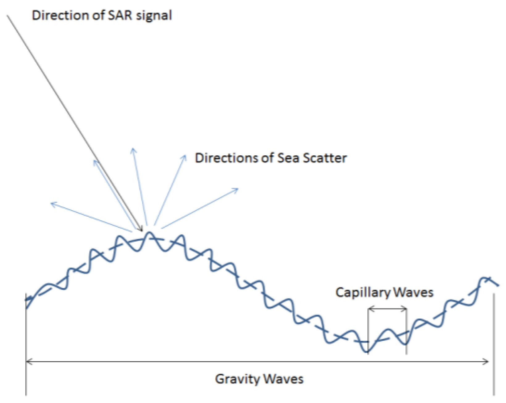
In SAR images, the detection of oil slick on the sea surface relies on the detection/quantification of its attenuation of Bragg scattering on the sea surface. When Bragg scattering happens, the signals from different sea surface facets interfere with each other. Moreover, according to the composite sea surface model, the roughness of the sea surface can be seen as small-scale capillary waves (contributing to Bragg scattering) superimposed on large-scale gravity waves. An illustration of this model can be seen in Figure 1. The sea surface of the oil-covered region appears smoother than its surrounding area. This is because the Bragg scattering of these areas is suppressed by the presence of hydrocarbons. However, the main backscatter from the sea surface is contributed by Bragg scattering. As a result, in SAR images the oil slick-covered area can usually be detected as a very dark (low backscattered) area.

In SAR images, the backscattered signal from oil spill is very similar to that from other ocean phenomena called “look-alikes” [1]. In recent years it has been demonstrated by theoretical and experimental studies the benefit of the polarimetric SAR paradigm, which explore the polarimetric SAR measurements and a proper electromagnetic modelling to distinguish light-damping surfactants from heavy-damping ones. This can be exploited as one case to sort out most of the look-alikes that are typical, such as biogenic films (slicks that are produced by marine organisms, such as fishes, algae, etc.), which normally cause very little harm to the marine environment [12,13].

The feasibility of polarimetric SAR-based oil spill classifications relies on the fact that the polarimetric mechanisms for oil-free and oil-covered sea surface are largely different [14]. Before the availability of polarimetric observations, hydrocarbons and biogenic slicks were difficult to distinguish because they damped the short gravity-capillary waves with almost the same strength [15]. However, based on different polarimetric scattering behaviors, hydrocarbons and biogenic slicks can now be better distinguished: for oil-covered areas, Bragg scattering is largely suppressed, and high polarimetric entropy can be documented. In the case of a biogenic slick, Bragg scattering is still dominant, but with a lower intensity. Thus, similar polarimetric behaviors as those of oil-free areas should be expected in the presence of biogenic films [3].

Despite being helpful to oil spill classifications, fully (or quad-) polarimetric SAR is facing the challenges of its system complexity and reduced swath width caused by the doubled pulse repetition frequency (PRF). To overcome this problem, dual polarimetric SAR systems, which transmit a single polarization signal, are often considered [16]. However, traditional dual polarimetric SAR systems transmitting only horizontal or vertical polarized signals have a limitation when acquiring the complete polarimetric behavior of selected targets.

Compared with conventional dual-polarimetric SAR modes, compact polarimetric (CP) SAR systems have higher sensitivity to the polarimetric behavior of some ground targets. Similarly, in CP SAR modes, the radar transmits only a linear combination of horizontal and vertical (π/4) or circularly (π/2, also called CTLR) polarized signals and linearly receives both horizontal and vertical polarizations. As a result, compact polarimetric SAR modes can be considered as special kinds of dual polarimetric SAR modes, and vice versa. Based on a general formalism of dual and compact polarimetric SAR data, a unified framework was proposed to analyze different CP SAR modes and its feature products [17].

Since the 2000s, CP SAR has become a new research trend [16,18,19]. In the years following the development of this technique, most studies focused on the applications of land monitoring, e.g., biomass and soil moisture estimation [20]. Recently, it began to be considered in maritime surveillance applications [21,22,23].

In data received via CP SAR modes, Stokes parameters and covariance matrices can be calculated from the measurement vector of SAR data, and further polarimetric analysis can be employed [24]. Some important polarimetric parameters, such as the degree of polarization (DoP), relative phase, entropy, anisotropy and α, can also be derived [22,25,26]. It is noted that the processing method and definitions of some parameters for CP SAR data, in the process of calibration, decomposition and classification, can be different.

Some previous studies explored the possibility of taking advantage of dual- and compact polarimetric SAR data to classify oil spills and biogenic slicks [27,28,29]. However, there are seldom quantitative comparisons of different polarimetric SAR modes, and their performance for actual oil spill classification applications. One important benefit of Pol-SAR paradigm is its robustness, i.e., it successfully works with airborne and spaceborne SARs and for different frequencies. Due to the fine classification capability of polarimetric features, polarimetric SAR-based methods may work on a wider range of sea status (surface wind and currents). However, because of the complexity of sea surface polarimetric scattering mechanisms, it is unrealistic to consider using any single characteristic to distinguish a variety of kinds of oil spills under different conditions. As a result, a synthetic and proper use of the polarimetric characteristics is the key to the accurate detection and successful interpretation of oil slicks. Moreover, the optimum compact polarimetric SAR mode varies with the different scattering behavior of the targets and also depends on specific classification tasks. Hence, in this study, we compare the oil spill detection using quad-, dual- and compact polarimetric features using supervised oil spill classifications. The study mainly concentrated on: (a) investigating the feature selection from quad- and compact polarimetric SAR data; (b) testing the performance of these features using several supervised classification algorithms, and (c) comparing SAR data from these modes to achieve marine oil spill classifications.

2. Methods

2.1. Quad-Polarimetric SAR Mode

For quad-pol SAR data, the 2 × 2 scattering matrix is measured on the traditional linearly horizontal and vertical bases, which can be described by [30]:

$$S=\left(\begin{array}{cc}{S}_{HH}& S_{HV}\\ S_{VH}& S_{VV}\end{array}\right)$$

(1)

where the subscript H and V describes the transmitted and received polarization, respectively, with H denoting horizontal and V denoting vertical directions. For the monostatic case, the reciprocity always holds, which means that the two cross-polarized terms are identical, i.e., S_HV = S_VH.

The covariance matrix can be derived by:

$$C=\left(\begin{array}{ccc}\langle S_{HH}^2\rangle & \langle \sqrt{2}{S}_{HH}{S}_{HV}^{*}\rangle & \langle S_{HH}{S}_{VV}^{*}\rangle \\ \langle \sqrt{2}{S}_{HV}{S}_{HH}^{*}\rangle & \langle 2S_{HV}^2\rangle & \langle \sqrt{2}{S}_{HV}{S}_{VV}^{*}\rangle \\ \langle S_{VV}{S}_{HH}^{*}\rangle & \langle \sqrt{2}{S}_{VV}{S}_{HV}^{*}\rangle & \langle S_{VV}^2\rangle \end{array}\right)$$

(2)

where * is the symbol of conjugate and “< >” stands for multilook by using an averaging window (5 × 5 in this study). This 5 × 5 averaging window is important to obtain the statistical property of the compound target’s polarization status and reduce the effect of speckle noise.

2.2. Feature Extraction from Quad-Polarimetric SAR Data

2.2.1. Single Polarimetric Intensity

The intensity of co-polarized channel is largely used in single polarimetric SAR-based oil spill detection algorithms. In this study, $S_{VV}^2$ is considered as one of the features for its higher SNRs compared to $S_{HH}^2$ on the sea surface. The hydrocarbons on the sea surface damp the short gravity and capillary waves of the sea surface, and hence, they are usually observed as very low backscatter areas. However, very similar dark areas can also be observed from SAR images when other kinds of oil are present, such as biogenic slicks.

2.2.2. H/α Decomposition Parameters

In 1997, Cloude and Pottier proposed a polarimetric information extraction method based on the decomposition of the 3 × 3 coherency matrix (3) of the target [31]:

$$T=U_3\left[\begin{array}{ccc}{\lambda }_1& & \\ & {\lambda }_2& \\ & & {\lambda }_3\end{array}\right]U_3^H$$

(3)

where H stands for transpose conjugate, and U₃ can be parameterized by Equation (4):

$$U_3=\left[\begin{array}{ccc}\cos ({\alpha }_1)e^{j{\varphi }_1}& \cos ({\alpha }_2)e^{j{\varphi }_2}& \cos ({\alpha }_3)e^{j{\varphi }_3}\\ \cos ({\alpha }_1)\cos ({\beta }_1)e^{j{\delta }_1}& \sin ({\alpha }_2)\cos ({\beta }_2)e^{j{\delta }_2}& \sin ({\alpha }_3)\cos ({\beta }_3)e^{j{\delta }_3}\\ \sin ({\alpha }_1)\sin ({\beta }_1)e^{j{\gamma }_1}& \sin ({\alpha }_2)\sin ({\beta }_2)e^{j{\gamma }_2}& \sin ({\alpha }_3)\cos ({\beta }_3)e^{j{\gamma }_3}\end{array}\right]$$

(4)

The three eigenvalues of the coherency matrix T are real numbers, arranged as ${\lambda }_1>{\lambda }_2>{\lambda }_3$, U₃ is the unitary matrix, whose column vectors ${\overrightarrow{u}}_1$, ${\overrightarrow{u}}_2$ and ${\overrightarrow{u}}_3$ are the eigenvectors of T:

$$T={\displaystyle \sum _{i-1}^3{\lambda }_1}{\overrightarrow{u}}_1\cdot {\overrightarrow{u}}_1^H+{\lambda }_2{\overrightarrow{u}}_2\cdot {\overrightarrow{u}}_2^H+{\lambda }_3{\overrightarrow{u}}_3\cdot {\overrightarrow{u}}_3^H$$

(5)

The probability of three eigenvectors can be calculated by:

$$P_i=\frac{{\lambda }_i}{{\displaystyle \sum _{j=1}^3{\lambda }_j}}$$

(6)

The polarimetric entropy, which describes the randomness of the scattering mechanisms, can be defined as:

$$H=-{\displaystyle \sum _{i=1}^3{P}_i}{\log }_3(P_i)$$

(7)

The mean scattering angle α is defined by:

$$\alpha =P_1{\alpha }_1+P_2{\alpha }_2+P_3{\alpha }_3$$

(8)

The entropy H is a measure of the randomness of the scatter mechanism. It is base-invariant and closely related to eigenvalue λ, which represents different components of the total scatter power. For a clean sea surface, Bragg scattering dominates, so H is close to 0. In contrast, for oil slick-covered areas, the scattering mechanism becomes more complex; stronger random scattering results in higher entropy values. Moreover, for biogenic slicks, although the scattering power is lower, the main scattering mechanism is still Bragg, resulting in lower entropy compared to oil-covered areas. This way, H can be used to distinguish oil slicks and weak damping look-alikes.

Usually jointly used with H, the mean scattering angle α reflects the main scattering mechanism of the observed target. On slick-free sea surfaces, α is expected to be less than 45° as the Bragg scattering is dominant. In slick-covered regions, larger α can be measured, as a more complex scattering mechanism is present.

2.2.3. Degree of Polarization

Degree of polarization (DoP) is considered to be a very important parameter characterizing partially polarized EM waves. It can be derived from the Stokes vectors of any coherent radar modes, e.g., dual-pol, hybrid/compact and, of course, fully polarimetric SAR modes [32]:

$$P=\frac{\sqrt{g_{i1}^2+g_{i2}^2+g_{i3}^2}}{g_{i0}^2}={\left(1-4\frac{\left|{\mathsf{\Gamma }}_i\right|}{{(tr{\mathsf{\Gamma }}_i)}^2}\right)}^{\frac{1}{2}}$$

(9)

where g_i is Stokes vectors that can be used to describe both complete and partially polarized wave, and i stands for different polarization of transmission.

$$g=\left[\begin{array}{c}{g}_0\\ g_1\\ g_2\\ g_3\end{array}\right]=\left[\begin{array}{c}\langle {\left|E_v\right|}^2+{\left|E_h\right|}^2\rangle \\ \langle {\left|E_v\right|}^2-{\left|E_h\right|}^2\rangle \\ 2\mathrm{Re}\langle E_h{E}_v^{*}\rangle \\ 2\mathrm{Im}\langle E_h{E}_v^{*}\rangle \end{array}\right]$$

(10)

where E_v and E_h is vertically and horizontally received backscatter, respectively, and < > also stands for multilook by using an averaging window.

DoP measures to what extent the scattered wave is deterministic and can be described by a polarimetric ellipse with fixed parameters. On the Poincare sphere, it represents the distance between the last three components normalized Stokes vectors and the origin [32]. It is 1 for complete polarized waves and 0 for fully unpolarized waves. For clean sea surfaces and weak-damping areas, the scattering mechanism can be described by the Bragg scattering; as a result, the DoP is large. For hydrocarbon slicks, random scattering mechanisms are dominating, and much lower DoP are observed.

2.2.4. Ellipticity χ

Ellipticity χ describes the polarization status of the scattered EM wave. From the Stokes vector, it can be calculated by:

$$\sin (2\chi )=-\frac{s_3}{m{s}_0}$$

(11)

where m stands for the degree of polarization of the received EM wave.

The parameter χ can be employed as an indicator of the scattering mechanism. For slick-free sea surfaces where Bragg scattering is dominant, the sign of χ is negative. For oil-covered sea surfaces, as a more random scattering mechanism is present, χ will be larger and can become positive [28]. This feature makes χ a logical binary descriptor of slick-free vs. oil-covered areas.

2.2.5. Pedestal Height

Normalized radar cross-section (NRCS) σ⁰ measures how detectable an object is per unit area on the ground. In the co-polarized signature of the scene, the σ⁰ is a function of both the tilting angle Φ and the ellipticity χ of the polarization ellipse. The pedestal height (PH) is defined as the lowest value of all the σ⁰, plotted in the co-polarized signature. The PH describes the unpolarized energy of the total scattering power and behaves as a pedestal on which the co-polarized signature is set [14,33]. The normalized pedestal height (NPH) can be approximately calculated as the minimum eigenvalue divided by the maximum one:

$$NPH=\frac{\min ({\lambda }_1,{\lambda }_2,{\lambda }_3)}{\max ({\lambda }_1,{\lambda }_2,{\lambda }_3)}$$

(12)

For clean sea surfaces, the scattering mechanism is pure Bragg, so an NPH value close to 0 is expected. For an oil-covered area, however, much higher NPH can be expected due to the non-Bragg scattering that reflects a more diverted scattering mechanism.

2.2.6. Co-Polarized Phase Difference

The co-polarized phase difference (CPD) is defined as the phase difference between the HH and VV channels [3]:

$${\phi }_c={\phi }_{HH}-{\phi }_{VV}$$

(13)

From multilook SAR data, it can be also derived as:

$${\phi }_c=\arg (\langle S_{HH}{S}_{VV}^{*}\rangle )$$

(14)

where arg(*) stands for phase calculation.

The standard deviation of CPD has been proposed as a very efficient parameter indicating sea surface scattering mechanisms [3]. It can be estimated from ${\phi }_c$ using a sliding window. On slick-free sea surfaces, the HH-VV correlation is high, and a narrow CPD distribution is expected. This resulting CPD will have a small standard deviation, similarly for weak-damping surfactant-covered areas. In oil slicks where the Bragg scattering is weakened and other scattering mechanisms increase, the HH-VV correlation largely decrease. As a result, the CPD pdf becomes broader, and its standard deviation largely increases.

2.2.7. Conformity Coefficient

The conformity coefficient μ was firstly used in compact polarimetric SAR applications for soil moisture estimations (Freeman et al., 2008). In a fully polarimetric scheme, it can be approximated as [6]:

$$\mu \cong \frac{2(\mathrm{Re}(S_{HH}{S}_{VV}^{*})-{\left|S_{HV}\right|}^2)}{{\left|S_{HH}\right|}^2+2{\left|S_{HV}\right|}^2+{\left|S_{VV}\right|}^2}$$

(15)

The conformity coefficient μ evaluates whether surface scattering is the dominant among all the scattering mechanisms. For a slick-free sea surface, Bragg scattering results in a very small cross-pol power and high HH-VV correlations and $\mathrm{Re}(S_{HH}{S}_{VV}^{*})>{\left|S_{HV}\right|}^2$; hence, μ is positive. However, for hydrocarbon-covered areas, as non-Bragg scattering exists, HH-VV correlation is lower, and cross-pol component largely increases, which is very likely to have $\mathrm{Re}(S_{HH}{S}_{VV}^{*})<{\left|S_{HV}\right|}^2$; hence, μ is negative. For weak-damping cases, such as biogenic slicks, since Bragg scattering is still dominant, $\mathrm{Re}(S_{HH}{S}_{VV}^{*})>{\left|S_{HV}\right|}^2$ is still valid and results in positive μ. Under this rationale, conformity coefficients can be used to effectively distinguish hydrocarbon slicks from biogenic slicks.

2.2.8. Correlation and Coherence Coefficients

The correlation and coherence coefficients that are derived from the coherence matrix are also used for oil slick discrimination [34].

$${\rho }_{HH/VV}=\left|\frac{\langle S_{HH}{S}_{VV}^{*}\rangle }{\langle S_{HH}^2\rangle \langle S_{VV}^2\rangle }\right|$$

(16)

$$Coh=\frac{\left|\langle T_{12}\rangle \right|}{\sqrt{\langle T_{11}\rangle \langle T_{22}\rangle }}$$

(17)

where T_ij are elements of the coherence matrix T.

These two parameters both lie between 0 and 1. For a slick-free area, where Bragg scattering is dominant, HH and VV channels are highly correlatable, so they are expected to be very close to 1. For an oil-covered sea surface, a much lower HH/VV correlation is expected, so both the correlation and coherence coefficients are much lower.

The polarimetric SAR features above and their relative behaviors in the presence of different ocean surface targets are summarized in

Table 1. Behaviors of main polarimetric SAR features on different types of surfaces. DoP, degree of polarization; CPD, co-polarized phase difference.

Pol-SAR Features	Clean Sea Surface	Mineral Oil (Strong Damping)	Biogenic Slicks (Weak Damping)
Entropy (H)	Lower	High	Low
Alpha (α)	Lower	High	Low
DoP	High	Low	High
Ellipticity	Negative	Positive	Negative
Pedestal Height (PH)	Lower	High	Low
Std. CPD	Lower	High	Low
Conformity Coefficient	Positive	Negative	Positive
Correlation Coefficient	Higher	Low	High
Coherence Coefficient	Higher	Low	High
$S_{VV}^2$	High	Low	Low

Note: “lower” and “higher” means that the property of the feature on a certain type of surface is close to the other surface that has the property of “low” or “high”, but slightly lower or higher. “Std. CPD” stands for the standard deviation of CPD.

.

2.3. Dual- and Compact Polarimetric SAR Modes

Compact polarimetric SAR modes were proposed to solve the contradiction between polarimetric observation capabilities and the swath width, system complexity, power budget and data rate of the radar system. Actually, the idea of transmitting one polarized signal and coherently recording the backscattered signal in H and V polarimetric channels was considered by U.S. scientists as far back as 1960. In the 2000s, this operation mode was reconsidered by Souyris et al. [16] and was given the new name of “compact polarimetric” to differentiate from “fully polarimetric” or “quad-polarimetric”.

Dual polarimetric (DP) SAR systems transmit a horizontal (H) or a vertical (V) linearly-polarized signal and coherently record both horizontal and vertical polarized backscattered signals. They can be treated as a special kind of compact polarimetric SAR mode. In real applications, usually HH/HV or HV/VV dual polarization modes are used, for the reason that in these modes, only the H or V polarized signal is transmitted. However, on the sea surface, the backscatter of the cross-polarized channel (HV) is usually much lower than the co-polarized channels [34], sometimes close to the noise floor of the radar instruments. As a result, HH/HV dual polarimetric modes have limited performance on oil spill classification applications. Although there is no HH-VV dual polarimetric SAR operating, except a special experimental imaging mode of TerraSAR-X, this mode is considered for comparative analysis in this paper.

The 2D measurements vector $\overrightarrow{K}$ of HH/VV dual-polarized, π/2 and π/4 compact polarimetric SAR modes are provided in Equations (18)–(20), respectively:

$${\overrightarrow{K}}_{HHVV}=\left(\begin{array}{l}{S}_{HH}\\ S_{VV}\end{array}\right)$$

(18)

$${\overrightarrow{K}}_{pi/2}=\frac{1}{\sqrt{2}}\left(\begin{array}{c}{S}_{HH}-j{S}_{HV}\\ S_{HV}-j{S}_{VV}\end{array}\right)$$

(19)

$${\overrightarrow{K}}_{pi/4}=\frac{1}{\sqrt{2}}\left(\begin{array}{c}{S}_{HH}+S_{HV}\\ S_{HV}+S_{VV}\end{array}\right)$$

(20)

Table 2. Different polarimetric SAR modes.

	Receive	H	V	H and V (Incoherently)	H and V (Coherently)	R and L (Coherently)
Transmit
H		Single	Single	Alternating	Dual Pol	—
V		Single	Single	Alternating	Dual Pol	—
H and V		—	—	Alternating	—	—
45°		—	—	—	π/4 Compact
R/L		—	—	—	π/2 Compact (Hybrid)	Dual-circular (DCP)

Note: Blank means that at the present stage, there is not an operational SAR system with such a transmit/receive combination. R and L stand for right and left circular polarization, respectively.

lists several main polarimetric SAR modes, which can be differentiated by their different transmission and receiving polarimetric combinations.

The covariance matrix can also be used to reflect the second order statistics of the dual and compact polarimetric SAR data, which can be derived from their scattering matrix by:

$$C_{CP}=2\langle {\overrightarrow{K}}_{CP}{\overrightarrow{K}}_{CP}^{*}\rangle$$

(21)

where ${\overrightarrow{K}}_{CP}$ stands for measurements vector $\overrightarrow{K}$ of different dual- and compact polarimetric SAR modes.

2.4. Universal Feature Extraction from Dual- and Compact Polarimetric SAR Data

In order to explore polarimetric information, the following methods can be used to universally extract features from the measurements vectors of dual- and compact polarimetric SAR data. The features extracted from dual- and compact polarimetric modes shares similar characteristics as those derived from fully polarimetric mode, in the presence of a clean sea surface, hydrocarbons and biogenic films. Of course, some differences can also be observed between them for the reason that they carry different parts of the information of quad-pol SAR data. In the following part of this paper, they are compared and analyzed.

2.4.1. Elements in Measurement Vector $\overrightarrow{K}$

The elements of the measurement vector $\overrightarrow{K}$ of dual and compact polarimetric SAR modes can be derived from Equations (18)–(20):

$$\overrightarrow{K}={\left(\begin{array}{cc}{E}_H& E_V\end{array}\right)}^T$$

(22)

where T stands for the transpose.

Since for the sea surface, usually $S_{HV}^2$ is much smaller compared with the backscatter of co-polarized channels, $E_V^2$ represents close physical meaning to $S_{VV}^2$. It is selected as one of the features in classification experiments based on compact polarimetric SAR modes.

2.4.2. H/α Decomposition Parameters

Polarimetric entropy of CP SAR data can be directly calculated from the eigenvalues of the covariance matrix C_CP:

$$H={\displaystyle \sum _{i=1}^2-P_i}{\log }_2{P}_i$$

(23)

$$P_i=\frac{{\lambda }_i}{{\displaystyle \sum _j{\lambda }_i}}$$

(24)

Additionally, ${\lambda }_i$ (i = 1, 2) is the eigenvalue of coherency matrix C_CP. Entropy that is derived directly from CP SAR data has similar performance as that derived from quad-pol SAR data, in describing the complexity of the physical scattering mechanisms of targets.

Then, the mean scattering angle in CP SAR modes can be approximated by:

$$\alpha =P_1{\alpha }_1+P_2{\alpha }_2$$

(25)

where α_i can be derived from the eigenvector of the covariance of CP SAR data, similarly as in Section 2.2.

2.4.3. Degree of Polarization and Ellipticity

The degree of polarization and ellipticity can be similarly calculated from the Stokes vector of CP SAR mode, as introduced in Section 2.2.

2.4.4. Pedestal Height

Similarly, as in Section 2.2.5, pedestal height can be estimated from the eigenvalues of the covariance matrix of compact polarimetric SAR data by:

$$NPH=\frac{\min ({\lambda }_1,{\lambda }_2)}{\max ({\lambda }_1,{\lambda }_2)}$$

(26)

2.4.5. Co-Polarized Phase Difference

CPD can be proximately estimated from covariance matrix of CP SAR data by:

$${\phi }_{c(CP)}=\arg \left\{-i{E}_H{E}_V^{*}\right\}$$

(27)

Then, its standard deviation within a certain spatial window can be computed. In this paper, a window of 5 × 5 is applied.

2.4.6. Conformity Coefficient

Only for π/2 mode, the conformity coefficient is expressed as [6]:

$$Conf\cong \frac{2\mathrm{Im}(\langle E_H{E}_V^{*}\rangle )}{\langle E_H{E}_H^{*}\rangle +\langle E_V{E}_V^{*}\rangle }$$

(28)

2.4.7. Correlation Coefficient and Coherence Coefficient

Following the same rationale as in Section 2.2.8, the correlation coefficient in CP SAR mode can be defined as [6]:

$$Corr=\frac{\mathrm{Re}\left\{-i\langle E_H{E}_V^{*}\rangle \right\}}{\sqrt{\langle {\left|E_H\right|}^2\rangle \langle {\left|E_V\right|}^2\rangle }}$$

(29)

Additionally, for CP SAR modes, the coherency coefficient can be derived by:

$$Coh=\frac{\left|D_{12}\right|}{\sqrt{D_{11}{D}_{22}}}$$

(30)

where the coherency matrix D for dual- and compact polarimetric SAR modes can be defined as:

$$D=\left(\begin{array}{cc}{\langle E_H+i{E}_V\rangle }^2& \langle E_H+i{E}_V\rangle {\langle E_H-i{E}_V\rangle }^{*}\\ {\langle E_H+i{E}_V\rangle }^{*}\langle E_H-i{E}_V\rangle & {\langle E_H-i{E}_V\rangle }^2\end{array}\right)$$

(31)

2.5. Supervised Classifications

Supervised classifications can take advantage of training data samples to set up the decision rule for classification, which has the best capability of fitting training datasets, as well as predicting the class of testing data samples. In this paper, three largely used supervised classifiers are considered.

2.5.1. Support Vector Machine (SVM)

SVM is based on structural risk minimization, the basic idea of which is to map multi-dimensional feature into a higher dimensional space and use a hyperplane to separate them linearly with the maximum margin between different classes [35]. SVM has superb performance in dealing with classification problems with a small number of training datasets. It firstly maps training vectors x_i into a higher dimensional space by using kernel function Φ and, hence, finds a linear separating hyperplane with the maximal margin in this higher dimensional space. In this paper, the radial basis function is adopted as the kernel function.

2.5.2. Artificial Neural Network (ANN)

ANN was designed based on the nervous systems of animals [36]. It can be used to estimate the complicated unknown functions based on a large number of inputs. ANNs are often used for supervised classification for their adaptive nature. They can often obtain good performance when the training samples are sufficient. In this paper, the feed-forward neural network (FFNN) with three layers is considered. In the FFNN, each neuron (or call “unit”) contains a transfer function. The neuron of the hidden and output units performs the nonlinear sigmoid function, while the input units have an identity transfer function. Then, layers are connected to each other by a system of weights, which multiplicatively scale the values traversing the links. The weights and bias of these links in the network is firstly randomly initiated and then fine-tuned through the backpropagation process.

2.5.3. Maximum Likelihood Classification (ML)

ML is a kind of classical classifier that is widely used in a variety of remote sensing applications. Based on training data, the maximum likelihood method selects the set of values of the model parameters that maximizes the likelihood function [37].

2.6. Features Selection Scheme

In a classification scheme, continuously adding features generates the well-known pattern recognition problem known as the “curse of dimensionality”, which means that the classification performance will not always improve with the increase of added features, especially when the number of training data samples is limited. Sometimes, “bad” features may even largely lower the classification accuracy. Moreover, the increase of the number of features makes the classification algorithms time consuming. In this paper, a forward feature selection scheme is considered, to choose the optimum feature sets for each classifier: starting from the best 2 features, the classification chooses to add the feature that provides the largest improvement on classification accuracy at each time. Then, in the comprehensive analysis, feature sets that achieved the best classification performance are employed.

2.7. Classification Accuracy Evaluation

In this study, overall accuracy (OA) and kappa coefficients (Kappa) are employed to quantitatively evaluate the classification accuracy. They can be derived from the confusion matrix of the testing data samples, where the rows represent the classified results and columns represent the referenced data. In the confusion matrix, the last row is the sum of all previous rows, and the last column is the sum of all previous columns. The OA is calculated by summing the number of pixels classified correctly divided by the total number of pixels, and the kappa coefficient measures the accuracy of the classification in another way; the definitions of both of them are shown below:

$$OA=\frac{{\displaystyle \sum _{i=1}^{n-1}{X}_{ii}}}{X_{nn}}$$

(32)

$$Kappa=\frac{X_{nn}{\displaystyle \sum _{i=1}^{n-1}{X}_{ii}-{\displaystyle \sum _{i=1}^{n-1}(X_{in}{X}_{ni})}}}{X_{nn}^2-{\displaystyle \sum _{i=1}^{n-1}(X_{in}{X}_{ni})}}$$

(33)

where $X={\left\{x_{ij}\right\}}_{n\times n}$ (i, j = 1, 2, 3, …, n) is the confusion matrix and $X_{in}$ stands for the number of samples that belongs to the i-th class and classified as n-th class.

2.8. Dimension Reduction

Various features can be extracted from polarimetric SAR data. However, inevitably, they are correlated and suffer from noise. In this study, three typical algorithms, principle component analysis (PCA), local linear embedding (LLE) and ISOMAP, were comparatively employed to reduce the dimension of polarimetric SAR features.

PCA reduces the number of features by replacing them with their linear combination. These new features are derived by the idea of maximizing their variance and making them uncorrelated. It comes from the theory of linear algebra; PCA has been abundantly used in many applications and has become a very popular method for its highly efficient, non-parametric characteristic.

LLE is an unsupervised learning algorithm that computes low-dimensional, neighborhood-preserving embeddings of high-dimensional inputs. It maps its inputs into a single global coordinate system of lower dimensionality, and its optimizations do not involve local minima. LLE is capable of learning the global structure of nonlinear manifolds based on the exploration of the local symmetries of linear reconstructions [38].

ISOMAP takes advantage of local metric information by measuring geodesic distances and learning the underlying global geometry of a dataset. Developed from multidimensional scaling (MDS), it is capable of discovering the nonlinear degrees of freedom that underlie complex natural observations, such as human handwriting or images of a face under different viewing conditions [39].

3. Results

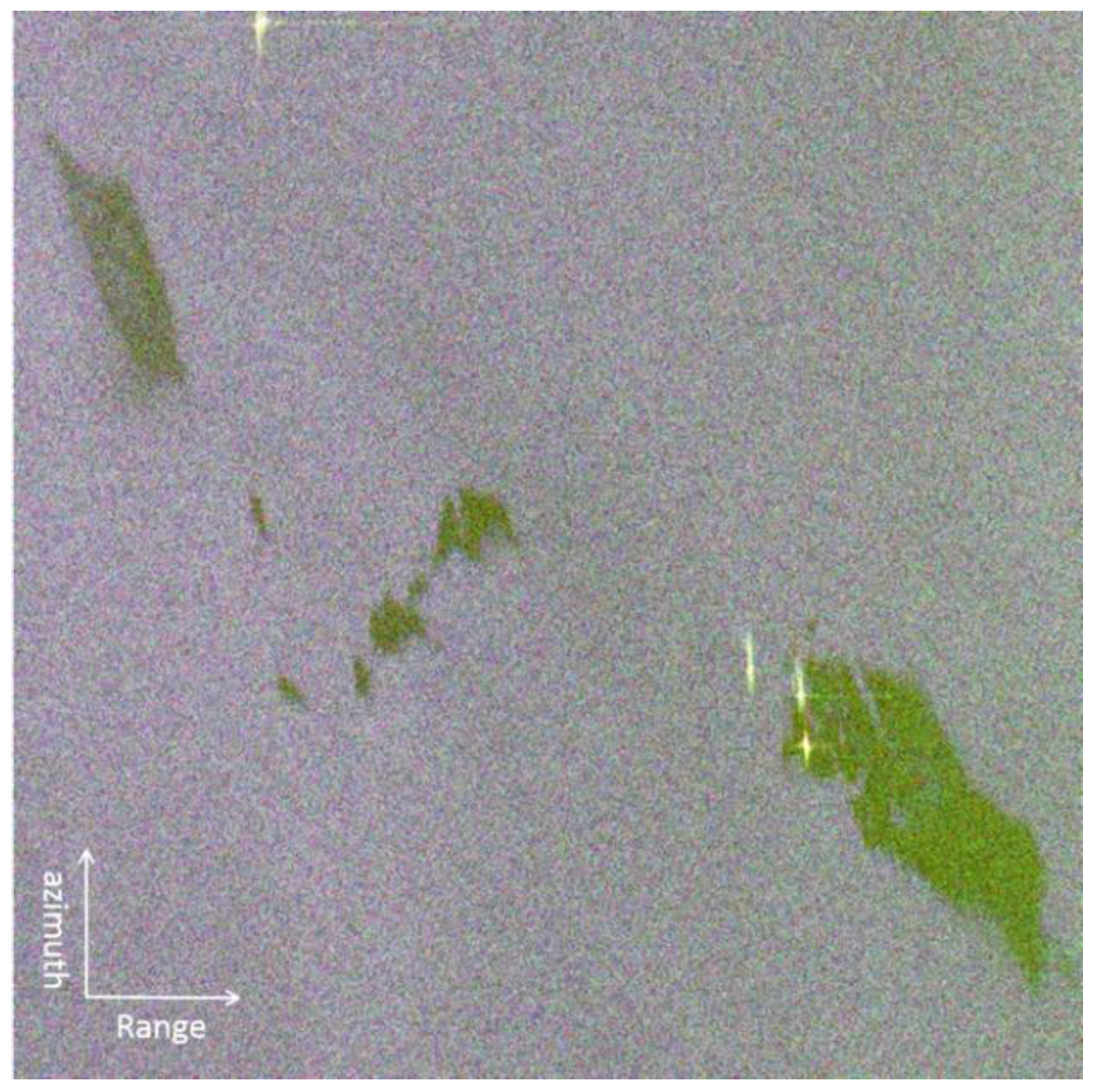
In this study, features extracted from RADARSAT-2 quad-pol SAR data were analyzed. The pseudo RGB image of the Radarsat-2 data on the Pauli basis are provided in Figure 2. It was acquired during the 2011 Norwegian oil-on-water experiment, in which three verified slicks were present; from left to right, they were: biogenic film, emulsions and mineral oil [34]. The biogenic film was simulated by Radiagreen ebo plant oil. Emulsions were made of Oseberg blend crude oil mixed with 5% IFO380 (Intermediate Fuel Oil), released 5 h before the radar acquisition. Additionally, the Balder crude oil was released 9 h before the radar acquisition [34].

In this study, the effect of feature numbers on the final classification result is analyzed, by considering three major supervised classifiers, namely, SVM, ANN and ML. Based on the quad-pol SAR data, dual-pol and compact polarimetric SAR data were also simulated, then features were extracted based on uniform feature extraction algorithms. Before the process of supervised classification, all of the features were normalized to the range of 0–1. Finally, the performance of features extracted from different polarimetric SAR modes in oil spill classification are compared and analyzed.

In the supervised classification experiment, 5393 and 5467 pixels of mineral oil covered and non-covered (including clean sea surface and biogenic films) training samples were picked within the study area respectively. Then, 5550 and 5535 testing samples of these two types are picked as the ground truth. The training and testing samples do not include each other. Both the training and testing sample include comparable numbers of pixels that are visually identified (based on ground truth) as clean sea surface, mineral oil and biogenic films (weak-damping surfactants).

3.1. Oil Spill Classification Based on Fully Polarimetric SAR Features

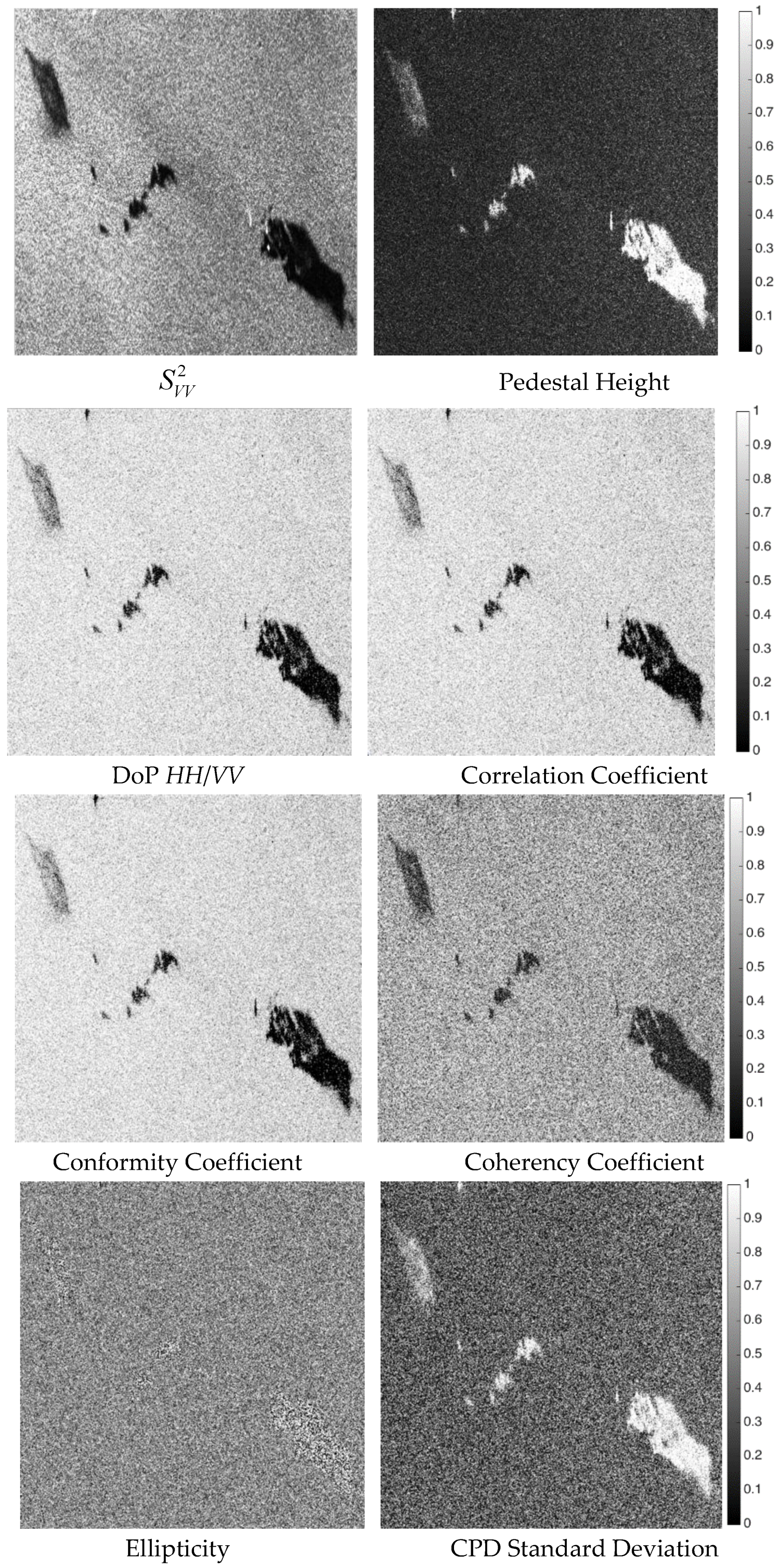
In the classification based on quad-pol SAR data, feature numbers from 2–10 are considered. The polarimetric features derived from quad-pol SAR data considered in the study are listed in

Table 3. Features that derived from quad-polarimetric SAR data.

Number	Feature
1	$S_{VV}^2$
2	Pedestal Height
3	Entropy
4	DoPHHVV
5	Correlation Coefficient
6	Conformity Coefficient
7	Coherency Coefficient
8	Ellipticity χ
9	CPD Standard Deviation
10	Alpha Angle

Note: Features 4 and 8 were extracted from the Stokes vector considering the HH and VV channels.

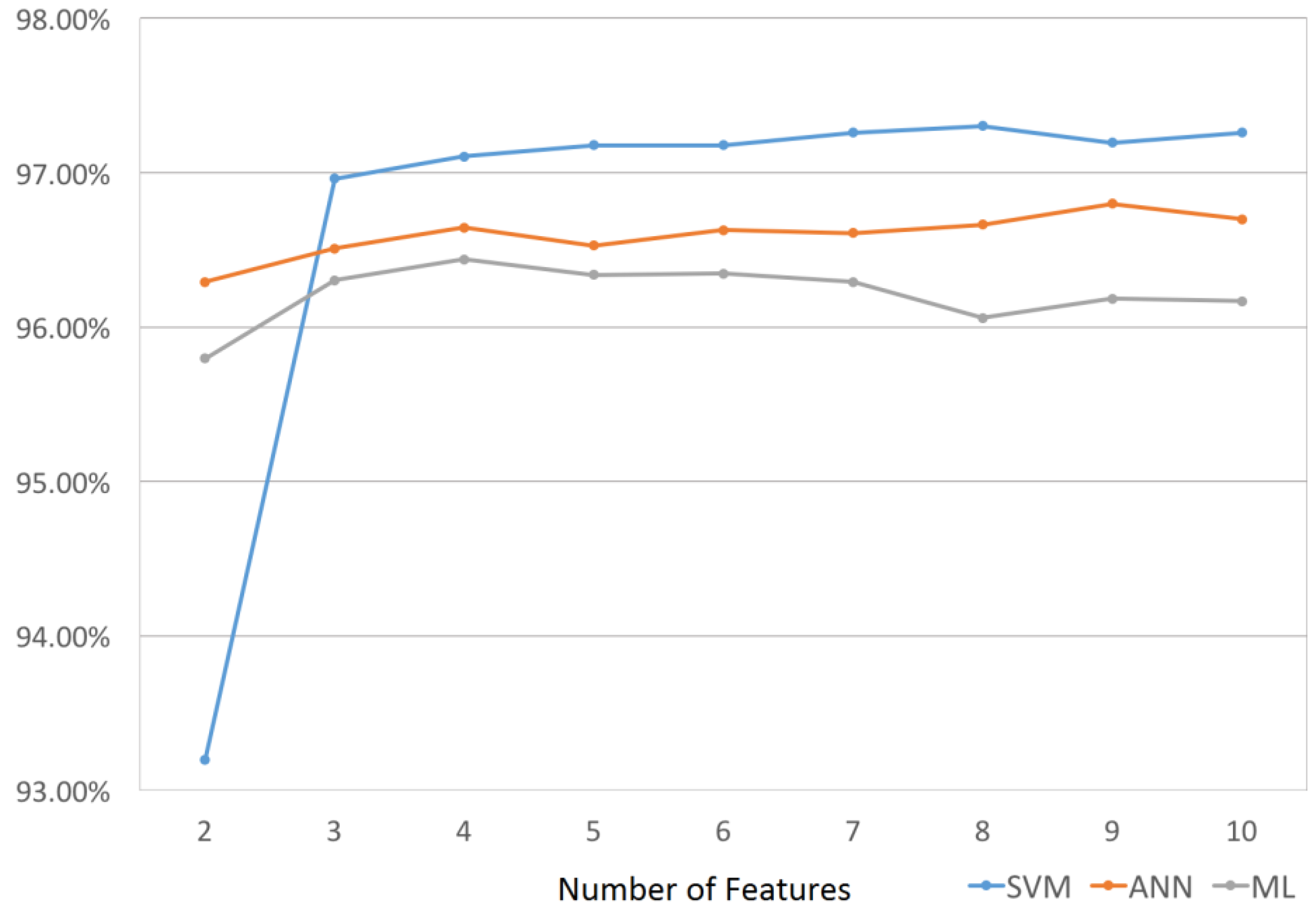
. All of the features considered in this experiment are provided in Figure 3. In the display, all of the features are normalized to [0, 1]. In Figure 4, the tendency of overall accuracy achieved by three classifiers is plotted. The best classification result was achieved when considering eight features for SVM, nine features for ANN and four features for MLC. Generally, SVM achieved the best classification performance, followed by ANN. This result proved the superb capability of SVM in dealing with a large number of features. It can be observed that in all of the classifications, after the best four features have been introduced, the classification results began to fluctuate and did not change very much. These four features are: pedestal height, correlation coefficient, standard deviation of CPD and alpha angle. The eight features used for SVM classification are: $S_{VV}^2$, pedestal height, entropy, DoP_HHVV, correlation coefficient, coherency coefficient, standard deviation of CPD and alpha angle. The nine features used for ANN are all of the features except ellipticity. As introduced in the previous session, all of these features have strong physical meaning, which enables them to largely contribute to the classification between mineral oil and clean sea surface/biogenic film. They are also not likely affected by the noise floor.

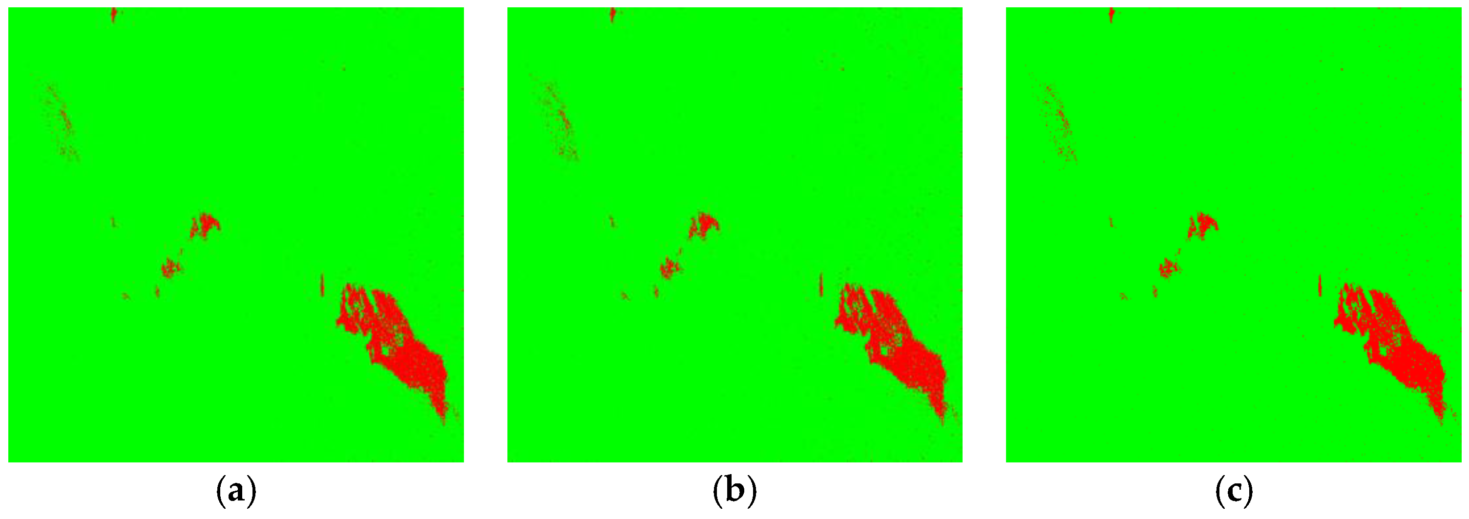
The best classification result was achieved by SVM with eight quad-polarimetric SAR features. This is shown in Figure 5a. Figure 5b,c demonstrates the classification results obtained by ML and ANN, respectively, where the red color indicates mineral oil and green indicates non-oil area. The confusion matrix of the best classification results achieved by these three classifiers is listed in

Table 4. Confusion matrix achieved by SVM based on 8 fully polarimetric features.

Class	Ground Truth (Pixels)
	Oil	Sea	Total
Oil	5429	178	5607
Sea	121	5357	5478
Total	5550	5535	11,085

Overall accuracy = 97.3027% (10,786/11,085), kappa coefficient = 0.9461.

,

Table 5. Confusion matrix achieved by ML based on 4 fully polarimetric features.

Class	Ground Truth (Pixels)
	Oil	Sea	Total
Oil	5411	256	5667
Sea	139	5279	5418
Total	5550	5535	11,085

Overall accuracy = 96.4366% (10,690/11,085), kappa coefficient = 0.9287.

and

Table 6. Confusion matrix achieved by ANN based on 9 fully polarimetric features.

Class	Ground Truth (Pixels)
	Oil	Sea	Total
Oil	5427	232	5659
Sea	123	5303	5426
Total	5550	5535	11,085

Overall accuracy = 96.7975% (10,730/11,085), kappa coefficient = 0.9359.

. From the detailed analysis on the confusion matrix of these classification results, it can be observed that the major reason that SVM is superior to the other two classifiers is that it successfully controlled the commission error of non-oil area, namely the error caused by wrongly classified clean sea surface and biogenic slicks.

3.2. Oil Spill Classification Based on Different Polarimetric SAR Modes

In this part, as listed in

Table 7. Uniform dual and compact polarimetric features considered in the study.

Number	Feature *
1	$E_V^2$
2	Pedestal Height (CP)
3	Entropy (CP)
4	DoP (CP)
5	Correlation Coefficient (CP)
6	Alpha Angle (CP)
7	Coherency Coefficient (CP)
8	Ellipticity χ (CP)
9	CPD Standard Deviation (CP)
10	Conformity Coefficient (π/2)

* Features 1–9 are extracted from dual and compact polarimetric SAR data following the methods introduced in Section 2.4, while Feature 10 is only available for π/2 mode. “CP” stands for features derived from compact polarimetric SAR data in order to distinguish them from those calculated from quad-pol SAR data.

, dual- and compact polarimetric SAR features are extracted from simulated SAR datasets (the conformity coefficient is only available in π/2 mode). The overall classification accuracy of three classifiers based on the features extracted from different polarimetric SAR modes is compared in Figure 6.

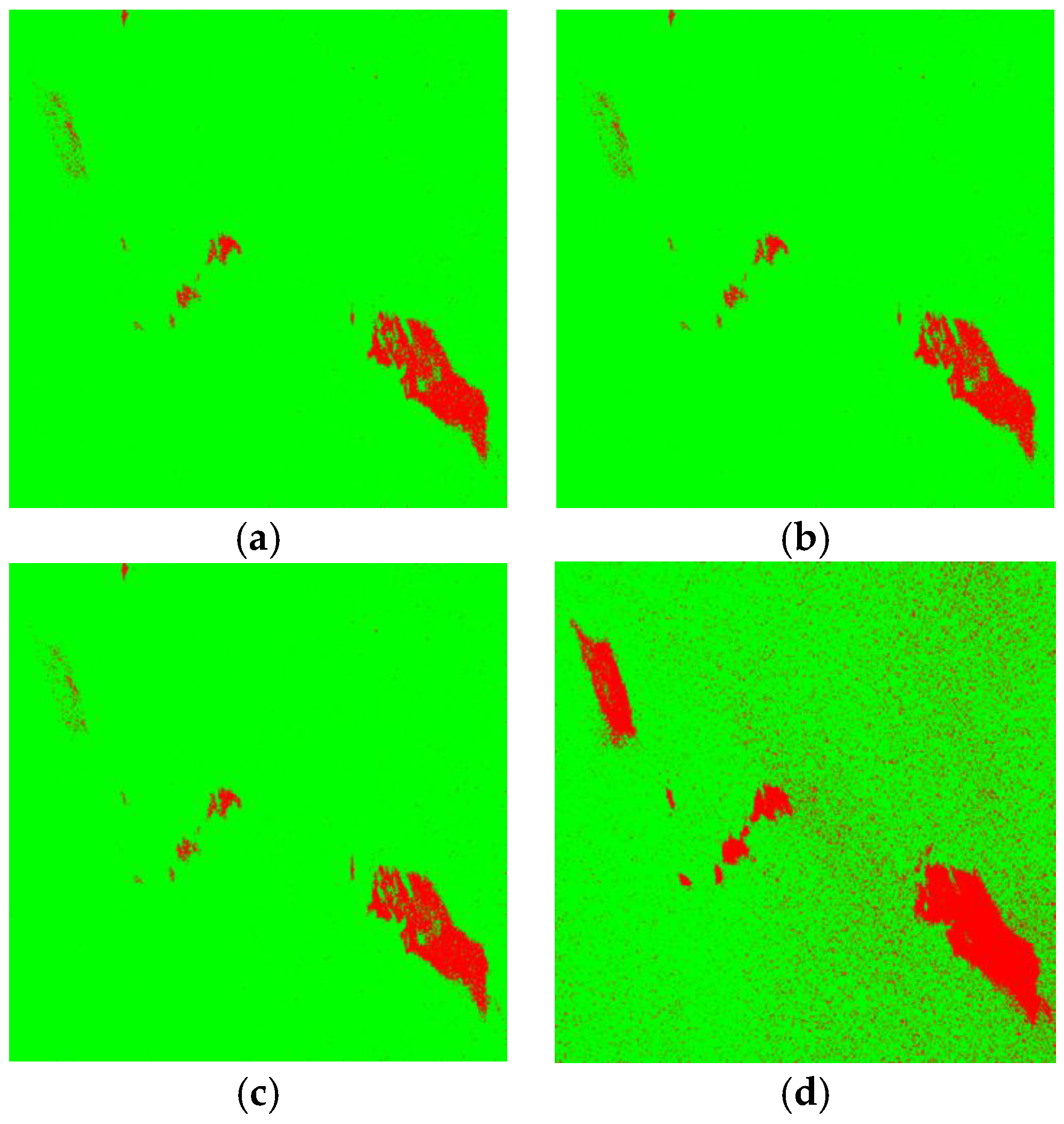
Quad-pol (QP) feature-based classification has the highest OA, followed by π/2 compact polarimetric SAR mode and HH/VV dual-polarized (DP) mode. π/4 mode-based classification has the lowest performance. In QP and π/2 modes, SVM achieved the best performance, while for HH/VV DP and π/4 modes, better performance was achieved by ML. Furthermore in dual- and compact polarimetric SAR modes, ML outperformed ANN; this may be explained by the fact that ANN has a higher requirement to the separability of the dataset and is more vulnerable to the loss or mixture of crucial information of the dataset. The confusion matrices of the classification results achieved by SVM based on features extracted from different polarimetric SAR modes are listed in

Table 8. Confusion matrix achieved by SVM based on 9 dual-polarized (DP) mode features.

Class	Ground Truth (Pixels)
	Oil	Sea	Total
Oil	5357	445	5802
Sea	193	5090	5283
Total	5550	5535	11,085

Overall accuracy = 94.2445% (10,447/11,085), kappa coefficient = 0.8849.

,

Table 9. Confusion matrix achieved by SVM based on 10π/2 mode features.

Class	Ground Truth (Pixels)
	Oil	Sea	Total
Oil	5378	363	5741
Sea	172	5172	5344
Total	5550	5535	11,085

Overall accuracy = 95.1737% (10,550/11,085), kappa coefficient = 0.9035.

and

Table 10. Confusion matrix achieved by SVM based on 9π/4 mode features.

Class	Ground Truth (Pixels)
	Oil	Sea	Total
Oil	5316	595	5911
Sea	234	4940	5174
Total	5550	5535	11,085

Overall accuracy = 92.5214% (10,256/11,085), kappa coefficient = 0.8504.

, with the feature number that achieved the best classification performance, and the classification results are demonstrated in Figure 7a–c.

Similar supervised classification experiments were also conducted based on single polarimetric feature $S_{VV}^2$ only. A much lower overall accuracy (61.7772%) and kappa coefficient (0.2348) were obtained. Figure 7d shows the classification result, from which it could be observed that most parts of the biogenic slick were misclassified to mineral oil. The confusion matrix (

Table 11. Confusion matrix achieved by SVM based on $S_{VV}^2$.

Class	Ground Truth (Pixels)
	Oil	Sea	Total
Oil	5438	4125	9563
Sea	112	1410	1522
Total	5550	5535	11,085

Overall accuracy = 61.7772% (6848/11,085), kappa coefficient = 0.2348.

) further supported this observation. This result manifested the limitation of single polarimetric SAR mode in distinguishing mineral oil and biogenic films.

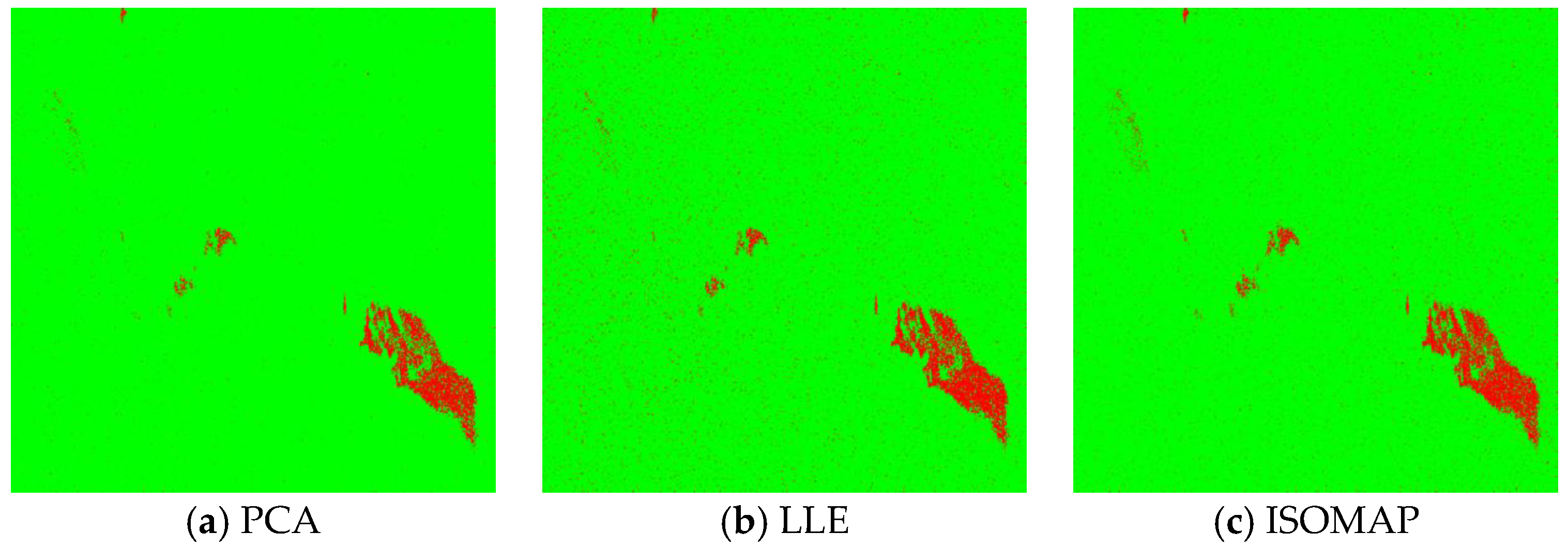
3.3. Oil Spill Classification Based on Dimension Reduction of Features

Based on the new feature sets, classification was conducted by using SVM. The classification results obtained by employing the three feature dimension reduction methods are shown in Figure 8.

Table 12. Confusion matrix achieved by SVM based on four features derived from PCA on quad-pol SAR features.

Class	Ground Truth (Pixels)
	Oil	Sea	Total
Oil	4649	82	4731
Sea	901	5453	6354
Total	5550	5535	11,085

Overall accuracy = 91.1322% (10,102/11,085), kappa coefficient = 0.8227.

,

Table 13. Confusion matrix achieved by SVM based on four features derived from local linear embedding (LLE) on quad-pol SAR features.

Class	Ground Truth (Pixels)
	Oil	Sea	Total
Oil	4879	197	5076
Sea	671	5338	6009
Total	5550	5535	11,085

Overall accuracy = 92.1696% (10,217/11,085), kappa coefficient = 0.8434.

and

Table 14. Confusion matrix achieved by SVM based on four features derived from ISOMAP on quad-pol SAR features.

Class	Ground Truth (Pixels)
	Oil	Sea	Total
Oil	4809	271	5080
Sea	741	5264	6005
Total	5550	5535	11,085

Overall accuracy = 90.8705% (10,073/11,085), kappa coefficient = 0.8174.

demonstrate the performance of classification. The feature set derived from LLE achieved the highest overall accuracy of 92.1696%. The feature set derived from PCA obtained an OA of 91.1322%, with the lowest false alarm rate. The feature set derived from ISOMAP had an OA of 90.8705%, which is the lowest among these three algorithms. Generally, feature reduction algorithms have acceptable performance in keeping the key information for distinguishing mineral oil and biogenic films. However, in this experiment, the performance achieved by dimension reduced feature sets is constantly lower than the original feature sets, which may be related to the issue of sample selection.

4. Discussion

With the help of polarimetric information, oil slicks and their biogenic films can be well separated. Experiments proved that the classification performance does not always increase with introducing more features; it fluctuates or decreases after the sufficient features are considered. This effect can be attributed to correlated and contradicting information carried in these features. In the demonstrated case, a set of four key features is sufficient, and the classification performance does not increase much when introducing more features. This phenomenon shows that most polarimetric information can be provided by several powerful and complementary features. As a result, in real applications, only a few representative features need to be extracted to save computing time and avoid the problem of “curse of dimensionality”.

In this study, we present a comparative study on features extracted from different polarimetric SAR modes to provide valuable information for oil spill classification. It was proven that quad-pol features have the highest overall accuracy, while π/2 compact polarimetric SAR modes had the best performance among all compact and dual-polarimetric SAR modes, followed by HH/VV dual-polarimetric SAR modes. The lowest performance was achieved by π/4 mode. In π/2 mode, the circularly-polarized signal is transmitted, which has been proven to be more suitable for a series of marine remote sensing applications [6,23], since it is very sensitive to the change of scattering mechanisms on the sea surface. HH-VV phase correlation is very helpful for distinguishing marine oil spill and biogenic oil slicks [3], and thus, HH/VV dual-polarization mode achieved relatively good performance.

In fully and π/2 compact polarimetric modes when the separability of the features is high, SVM achieved the highest performance in comparison with other supervised classifiers. The advantage of SVM is its good capability of handling the problem of the “curse of dimensionality”. It has better performance in dealing with data of a high dimensional feature space in supervised classification applications, such as this illustrated case. For quad-pol feature-based classification, ANN performed slightly better than ML, and for other modes, ML performed better than ANN. A possible explanation is that ANN is very sensitive to the quality of features and has the trend of over-training when dealing with features with disturbance. Therefore, in compact and dual-polarimetric SAR modes, ML performs better than ANN, although the latter one is more sophisticated in its architecture.

This study shows that polarimetric SAR can distinguish mineral oil from biogenic slicks. An important result is that the identification of different oils (bunker oil, crude oil, petrochemical films) is very important for clean-up operations. Different oils have different physical/chemical properties, e.g., viscosity, density, evaporation rate, etc., and theoretically, a difference in these properties can be observed in polarimetric SAR images. However, currently, there is not enough valid data to support this latter postulate. This analysis can be made in the future.

It is important to analyze the behavior of weathering oil in polarimetric SAR images. Particularly, evaporation, emulsification and sinking are important related slick detections by SAR. Studies [40,41] indicate that the percentages of oil trapped, evaporated and at the surface vary with the type of oil spilt and with the location in which spills are firstly generated. In essence, the movement of oil, its original type/density and the time that leads to its emulsification/evaporation/sinking are variable in different oil spills. It is also considered crucial to understand the effects of emulsification and ocean-driven slick movement in the size(s) and distribution of oil slicks at the surface for environmental protection [42]. Hence, more detailed experiments should be made to quantitatively analyze the degree of degradation of an oil spill based on polarimetric SAR.

5. Conclusions

The Norwegian oil-on-water experiment in 2011 provided polarimetric SAR acquisition with verified oil spill and biogenic slicks on one scene of Radarsat-2 data. More quad-pol SAR data samples are being further collected to derive more detailed and convincing results in the near future studies.

The key findings of this comparative study can be summarized as follows:

• Polarimetric SAR features can be input into supervised algorithms to achieve reliable oil spill classification. For this dataset, a feature set with four features is sufficient for most polarimetric features based oil spill classifications. They are: pedestal height, correlation coefficient, standard deviation of CPD and alpha angle.
• Among all of the compact polarimetric SAR modes, π/2 mode has the best performance among all of the dual- and compact polarimetric SAR modes, for its sensitivity to different scattering mechanisms caused by mineral oil and biogenic look-alikes.
• Among all of the supervised classifiers, SVM outperforms other classifiers when sufficient polarimetric information can be obtained, such as quad-pol mode. ML performs better than other supervised classifiers when only incomplete polarimetric information is available, such as traditional dual-pol and π/4 mode.

The reasons for the unreliable results in feature reduction experiments may be attributed to insufficient data sampling when computing feature maps. The understanding of oil in the characteristics of polarimetric SAR imagery is key to optimize the processing procedures of automatic oil spill detection and classification algorithms.

In the near future, there will be more compact polarimetric SAR data available for marine surveillance applications. The polarimetric observation capabilities of these sensors will largely improve the efficiency and reliability of oil spill detection and any future classifications applications based on SAR data.