Article

Methodological Considerations of Using Thermoelectrics with Fin Heat Sinks for Cooling Applications

Faculty of Engineering and Green Technology, UniversitiTunku Abdul Rahman, Kampar 31900, Malaysia
*
Author to whom correspondence should be addressed.
Appl. Sci. 2017, 7(2), 62; https://doi.org/10.3390/app7020062
Submission received: 25 September 2016 / Revised: 5 December 2016 / Accepted: 4 January 2017 / Published: 7 February 2017

Abstract

:
An experimental investigation was conducted to evaluate the performance of a thermoelectric (TE) module fitted to a conventional fin heat sink with a similar sized heat source. Experiments were conducted with power inputs at 10 W and 20 W under natural convection (NC) and forced convection (FC) air cooling. The results showed that the use of the TE module is not effective under the NC cooling mode. With the present TE module employed, under FC cooling at 20 W, the applied voltage (Vte) to the TE module should be >4 V and at 10 W, it should be >1 V. A simple iterative method of predicting the hot side temperature of the TE module was presented. Agreement between predicted and experimental values was better than 2%.

1. Introduction

A thermoelectric (TE) module consists of a number of thermocouples connected electrically in series and thermally in parallel. TEs are used with fin heat sinks (FHS) to dissipate the heat to the atmosphere. During operation, heat is generated within the thermoelectric cooler (TEC) device due to the Joule heating effect. As a consequence more heat is transferred to the heat sink than absorbed from the heat source. Typical thermal cooling with an air-cooled FHS is shown in Figure 1a and a water-cooled plate heat sink in Figure 1b. Natural convection (NC) or forced convection (FC) by air could be employed. A typical FHS consists of a flat metal base with an array of cooling fins on top with aluminum or copper as the most common metals used. Thermal contact resistances occur at the interfacing metal contacts. In addition, thermal heat spreading resistance exists whenever there is a difference between the heat sink and heat source surface areas. As semiconductor chips become more powerful and compact, they require greater heat dissipation. Hence, more effective thermal cooling systems have to be devised. A thermal cooling device consisting of an air-cooled FHS coupled to a TE module is shown in Figure 2.
Thermal heat spreading has been investigated by various researchers. Lee et al. [1] investigated the spreading resistances of various flat rectangular plates with various surface heat transfer coefficients. They compared their simulations with other known existing theories and found that for relatively thick plates, the constriction thermal resistance is insensitive to plate thickness and Biot number. It was solely dependent upon the relative contact size between the heat sink and heat source. Simons [2] simulated thermal heat spreading resistance using exact partial differential heat transfer equations and compared them with those obtained by Lee et al. [1] using aluminum and copper flat plate heat spreaders and under forced convection air cooling. Hasan et al. [3], on the other hand, applied the conductive thermal interface material to reduce the resistance. Ellison [4] derived an exact three-dimensional solution to determine the maximum heat spreading resistance for rectangular heat sources centered on larger sized plane heat sinks. Muzychka et al. [5] presented a general solution based on the separation of variables method for the thermal spreading resistances of eccentric heat sources on a rectangular flux channel. General expressions of an isoflux rectangular source on the surface of finite isotropic and compound rectangular flux channels were presented, as well as the solution for the temperature at the surface of a rectangular flux channel.
An overview of applications of TE devices for thermal cooling could be found in Rowe [6], Riffat and Ma [7], and Lee [8]. Sasaki et al. [9] obtained hot side temperatures between 40 °C and 62 °C and cold side temperatures between 8.4 °C and 14.8 °C at a power input of less than 80 W with cascaded or stacked TEs. Uemura [10] presented a brief description of commercial TE modules and showed how graphs provided by manufacturers could be utilized to select a module for a specific application. Webb et al. [11] developed equations that connect heat loads with material properties of the TE module and the cold and hot side operating temperatures. They went on to determine the optimum heat sink resistances for a fixed set of operating conditions and considered various existing heat sink heat exchangers to meet the resistance requirement of the heat sink. Riffat and Ma [12] developed a computer model to show the relationship between the cooling and heating requirements and the optimum TE properties. Chein and Huang [13] presented a theoretical model to determine the performance of a TE device for electronic cooling by assuming values of the hot and cold junctions and then determined the resistance of micro-channel heat sinks. Kim et al. [14] presented a computer simulation for a thermosyphon heat sink. Huang et al. [15] designed a test rig to determine the physical properties of a TE module. These results were then used to determine the optimum design of a TE cooler system using a thermal resistance network model for the heat sink. Additionally, Palacios et al. [16] presented a methodology to extract TE internal parameters from information provided by performance curves to simulate the behavior of a commercial module for a TE power generation system. Vian, J.G. and Astrain [17] developed a heat exchanger for the cold side of a TE module.
It is apparent from the literature that the thermal performance of TE modules could be affected by the physical properties, e.g., the Seebeck coefficient, the electrical resistance, and the thermal conductivity in the cooling applications. This paper presents the empirical investigations on the performance of a thermoelectric cooler system and, subsequently, to evaluate the thermal cooling performance of a TE module fitted to a conventional FHS and cooled under NC and FC air cooling.

2. Materials and Methods

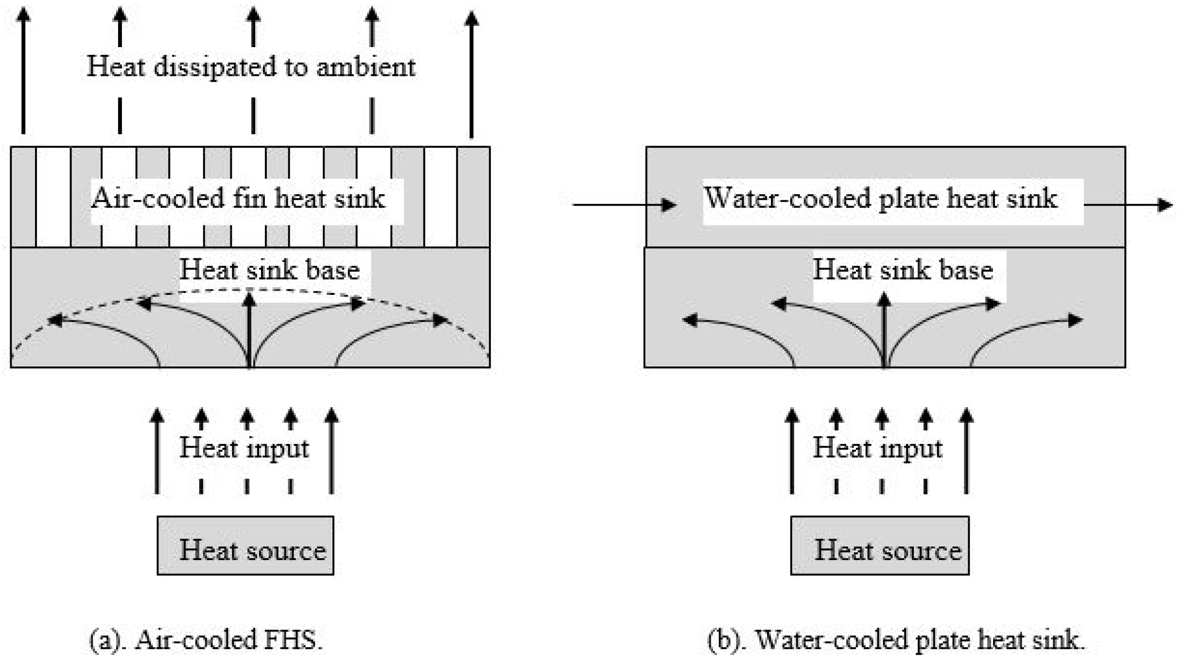
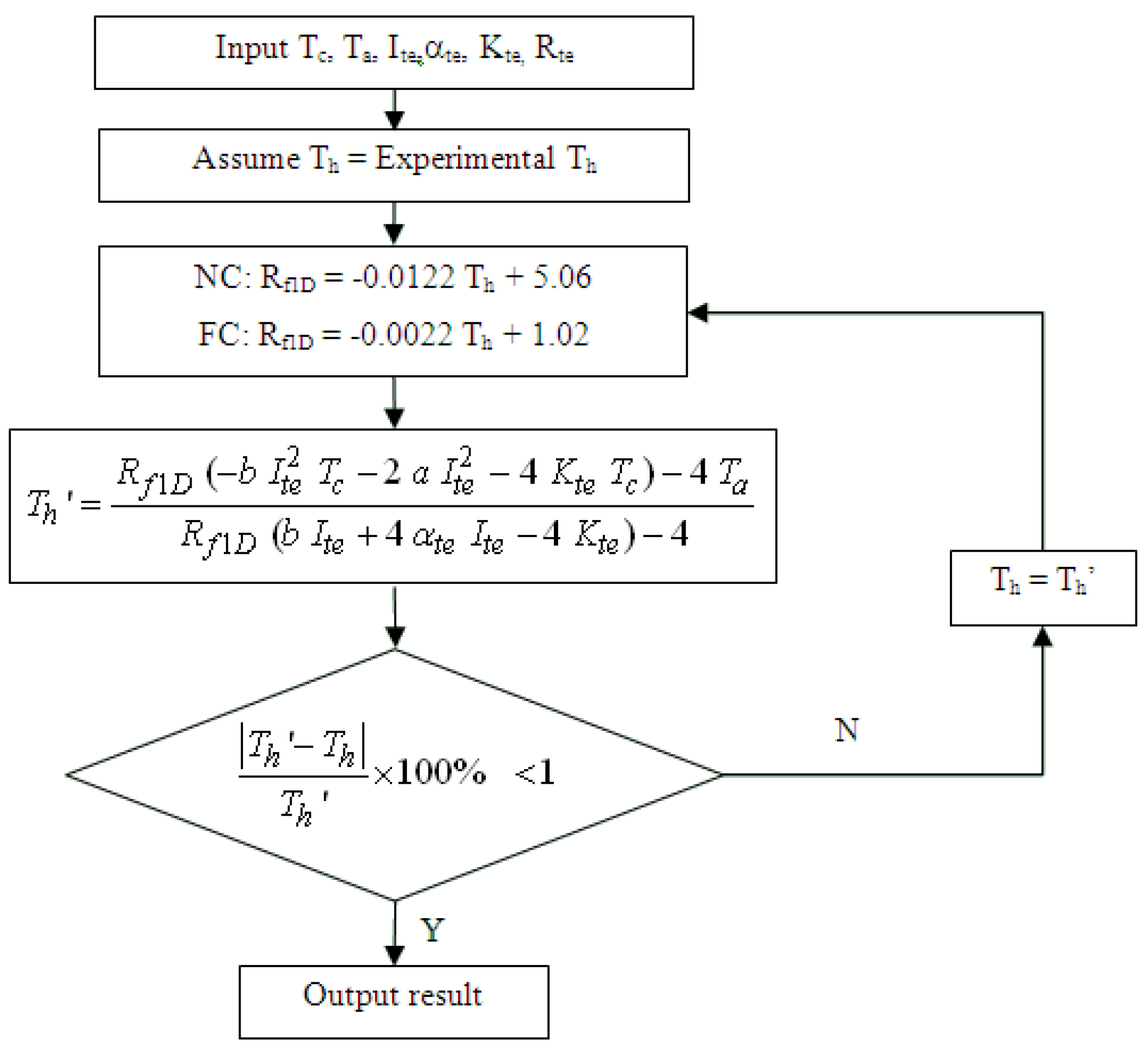
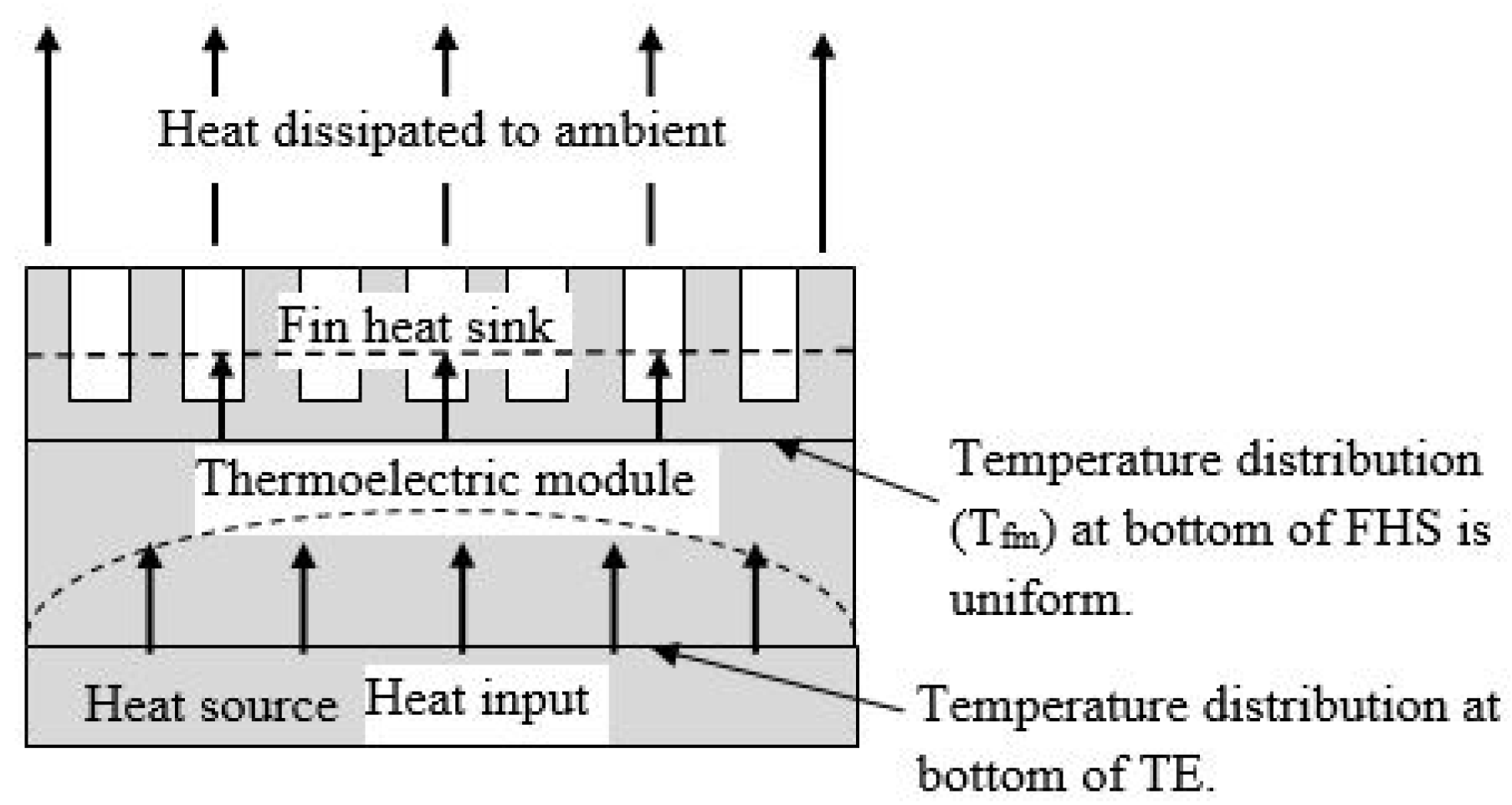
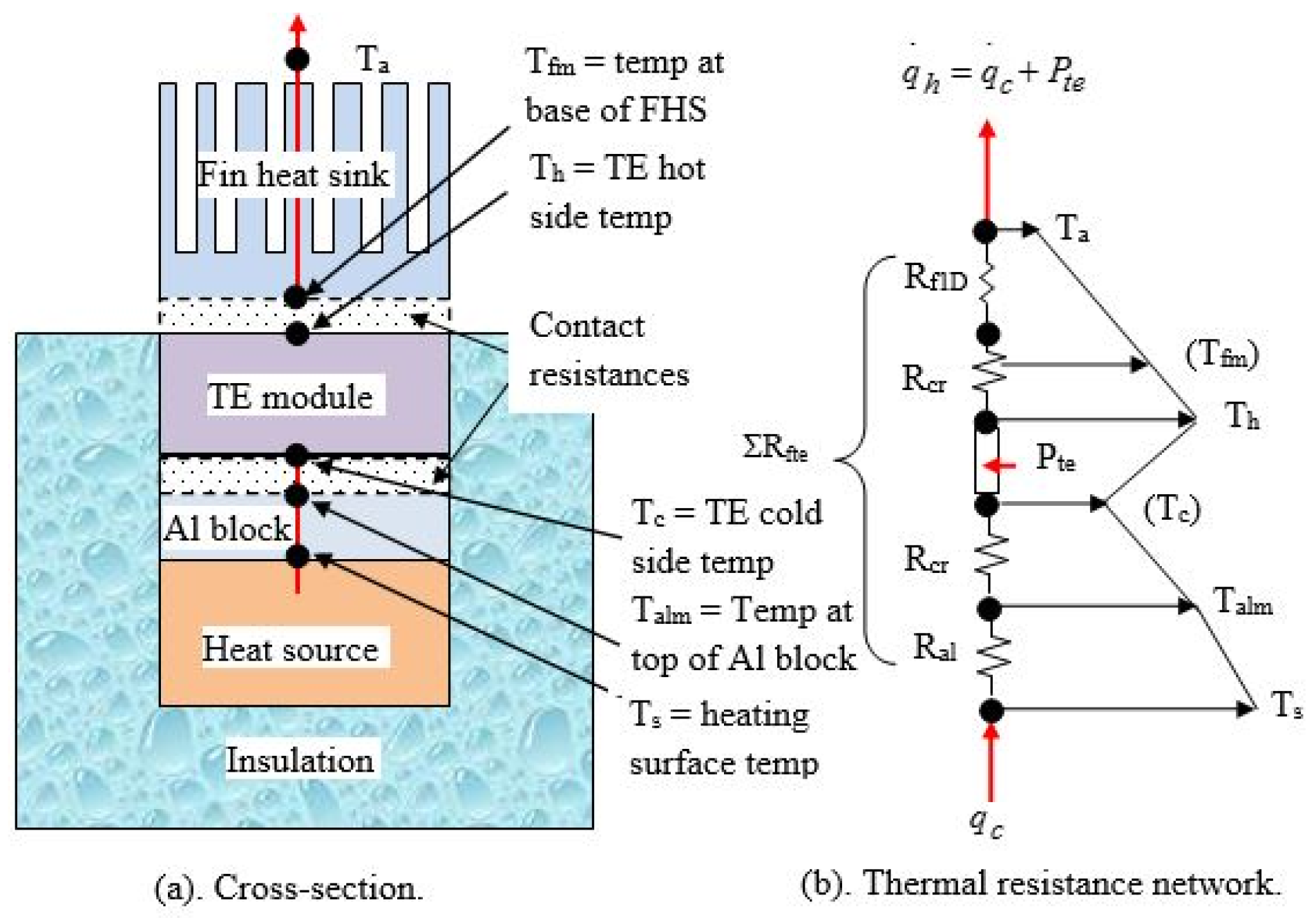
2.1. Thermal Resistance Model

Figure 3a shows a cross-section of the FHS-TE assembly. The TE module is sandwiched between a conventional FHS and a heat source. An aluminum block is added to the assembly to distribute the heat evenly from the heating element. The associated thermal resistance network is shown in Figure 3b. All interface temperatures are expected to be uniform since the heat flow is one-dimensional. Power (Pte) supplied to the TE module creates a low temperature at the cold side (Tc) of the TE and a high temperature (Th) at the hot side. Assuming perfect insulation as shown, heat absorbed at the cold side is equal to the heat supplied (PEH) from the heat source. Heat from the cold surface is dissipated at the hot surface.
The heat transfer rates at the cold (qc) and hot sides (qh) of the TE module are given by:
q c = α t e I t e T c 1 2 I t e 2 R t e K t e Δ T t e
and
q h = α t e I t e T h + 1 2 I t e 2 R t e K t e Δ T t e
Where αte, Ite, Rte, and Kte are the Seebeck coefficient, current, internal resistance, and thermal conductivity of TE, respectively. The temperature difference across the TE module is:
Δ T t e = T h T c
Where Th and Tc define the hot side temperature and cold side temperature of TE, respectively. An energy balance (Pte) gives the power to be supplied to the TE module:
P t e = q h q c = α t e I t e Δ T t e + I t e 2 R t e
The applied TE voltage (Vte) is:
V t e = α t e Δ T t e + I t e R t e
The cooling coefficient of performance of the TE is:
COP c = q c / P t e
In Figure 3b, the 1-D thermal resistance of the FHS is shown as Rf1D and the thermal resistance of the aluminum block as Ral. Contact thermal resistances Rcr between the aluminum block and TE module, as well as between TE and FHS, are assumed to be negligible. From the thermal resistance network the thermal resistance of the FHS is:
R f 1 D = ( T h T a ) / q h
Where Ta is the ambient temperature. The internal electrical resistance of the TE depends upon the mean operating temperature of the TE. This can be represented by:
R t e = a + b T m t e
Where a and b are constants in internal electrical resistance of TE. The mean TE temperature is calculated by:
T m t e = ( T h + T c ) / 2
From the above we obtain:
T h = R f 1 D ( b I t e 2 T c 2 a I t e 2 4 K t e T c ) 4 T a R f 1 D ( b I t e 2 + 4 α t e I t e 4 K t e ) 4
Figure 4 shows the flow chart to simulate the TE hot side temperature (Th) given the cold side temperature (Tc). The procedure involves an iteration process. Ambient (Ta) and cold side temperatures, and applied current (Ite) to the TE module are first specified together with the characteristics of the TE module, such as the Seebeck coefficient (αte), thermal conductance (Kte), internal electrical resistance (Rte), and the resistance constants a and b. From the manufacturer's datasheet, αte = 0.053 V/K, Kte = 0.66 W/K, Rte = 0.016, a = −0.36, and b = 0.006. First, a guessed value of Th is input into the program. Next, the simulated value of Th’ is calculated from Equation (10). The difference between the predicted and guessed values is then calculated. If the difference is more than 1%, the process is repeated until the difference is less than 1%. The thermal resistance Rf1D under NC and FC is then evaluated using the new value of Th’.

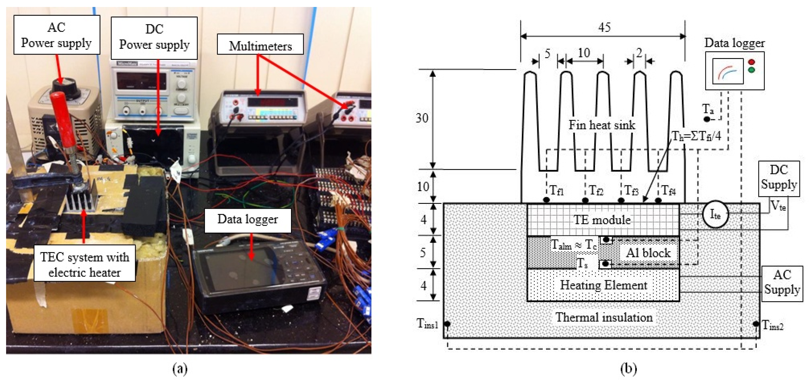
2.2. Experimental Procedure

An experimental apparatus to determine the thermal performance of a FHS-TE assembly is shown in Figure 5. The 40 mm × 40 mm × 4 mm thick TE module used is the HT8, 12, F2, 4040 manufactured by Laird Technologies (Penang, Malaysia). The five-fin aluminum FHS measured 45 mm × 45 mm, with a 10 mm thick base. The heating element measured 40 mm × 40 mm × 4 mm, and the aluminum block 40 mm × 40 mm × 5 mm. The electrical circuit for this is also shown. Thermal insulation was provided at the bottom and sides of the assembly up to, and including, the TE module to minimize heat loss to the ambient environment. The insulation consisted of a composite layer of 10 mm thick cork board (Trusco, Osaka, Japan) and 95 mm thick rockwool (Rockwool, Selangor, Malaysia). Heating was provided from an AC power supply (Shanghai MCP, Shanghai, China). Power to the heat source (PEH) was determined from the product of AC voltmeter (VEH) (GW Instek, Taipei, Taiwan) and ammeter (IEH) readings (GW Instek, Taipei, Taiwan). Power input to the TE (Pte) was determined from the product of DC voltmeter (Vte) (GW Instek, Taipei, Taiwan) and ammeter (Ite) readings (GW Instek, Taipei, Taiwan). Four thermocouples (Tf1–Tf4) (Graphtec, Tokyo, Japan) were inserted into 3-mm diameter holes drilled in a row through the base of the heat sink to measure the FHS/TE interface temperature distribution. TE hot surface temperature (Th) was obtained from the arithmetic mean of these four temperatures. Thermocouples centrally located in 1.5-mm deep grooves machined on the top and bottom surfaces of the aluminum block measured the mean cold surface temperature at the top of the aluminum block (Talm) and of the heating surface (Ts). The TE cold junction temperature (Tc) was assumed equal to Talm. The mean operating temperature (Tm) across the TE module was calculated by taking the arithmetic mean temperatures between hot (Th) and cold surfaces (Tc). Additional thermocouples were employed to measure the external surface temperature of the insulation (Tins) and ambient temperature (Ta). All thermocouples were connected to a data logger and logged every minute. Experiments were performed with heater power inputs at 10 W and 20 W (nominal). At each power input setting, experiments were carried out with increasing TE voltages from 1 V to 6 V. The results are tabulated in Table 1 for NC (Runs D1–D2) and for FC (Runs D3–D4).

3. Results and Discussion

Figure 6 and Figure 7 show the transient temperatures recorded for the hot (Th) and cold (Tc) sides of the TE and also for the heat source (Ts) surface temperature at a power input (PEH) of 10 W and under NC. The following results are observed:
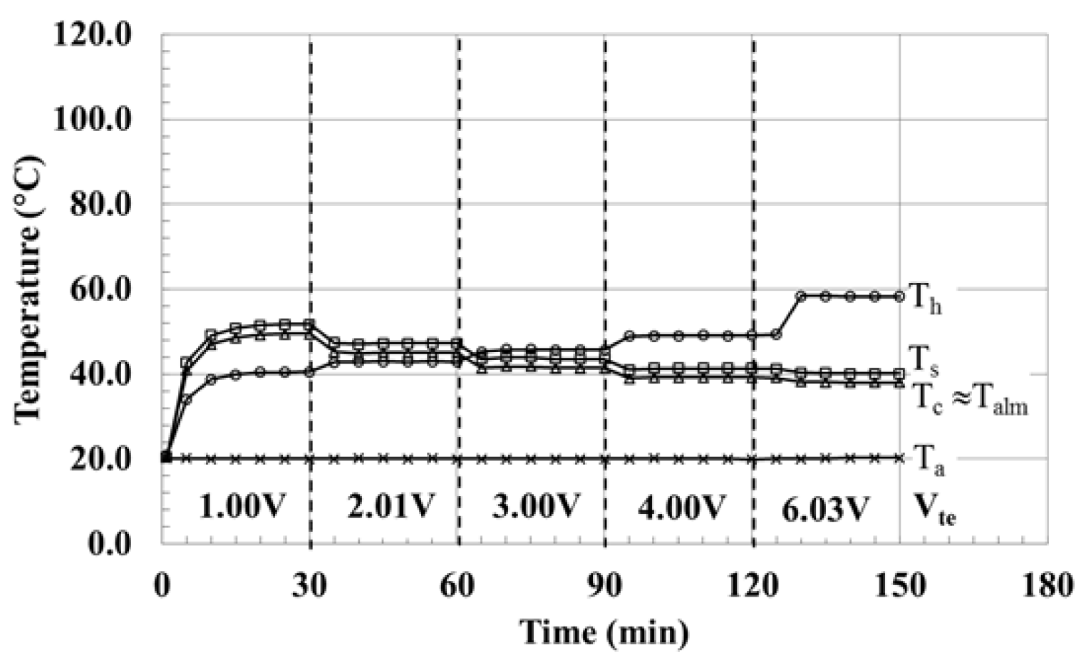
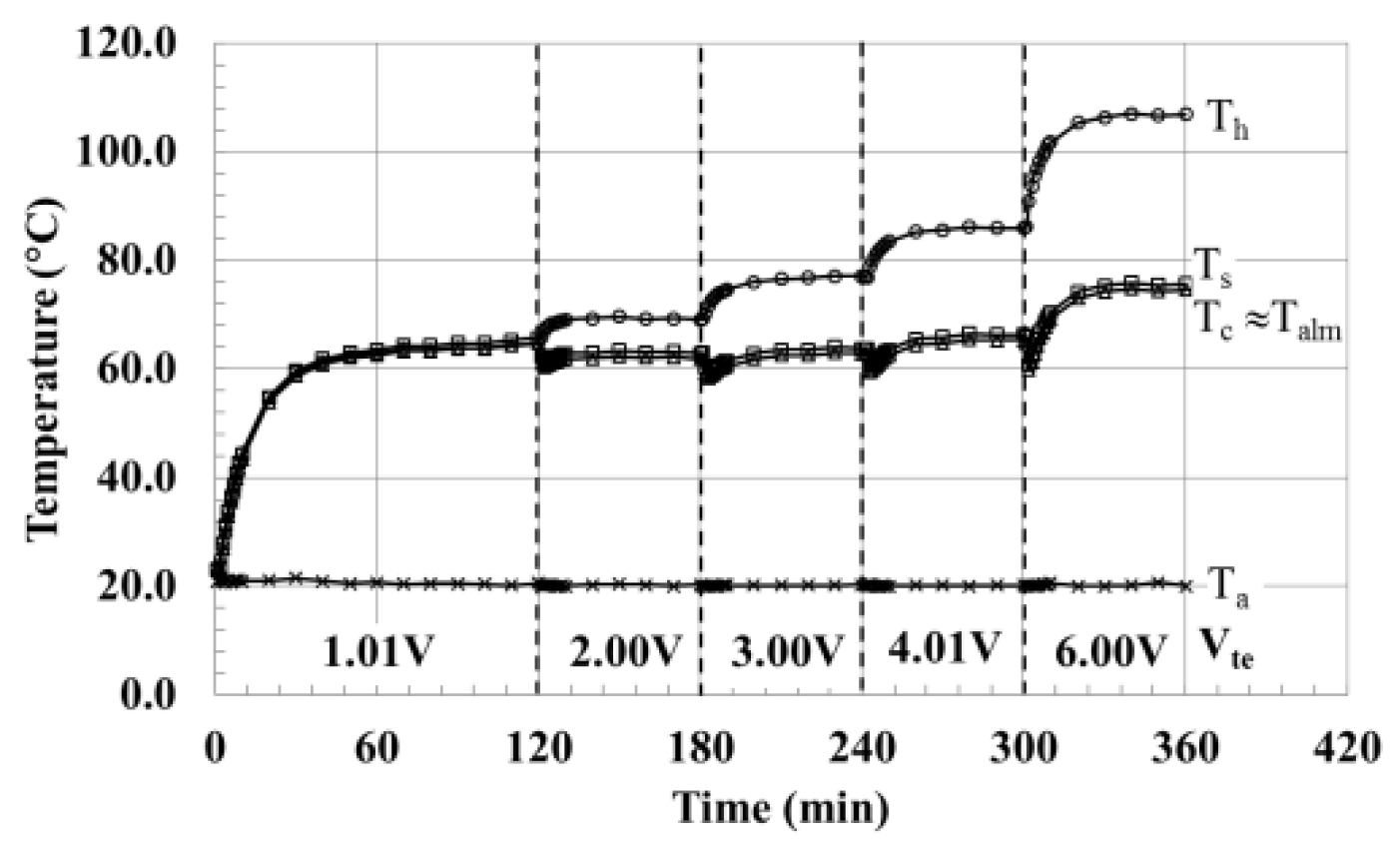
  • Temperatures of Th, Ts, and Tc are plotted for the first 120 min and, every 60 min thereafter. The results showed that steady state is achieved after 2 h at the low TE voltage run of 1 V while it took only about an hour at the higher TE voltage >2 V.
  • Heat source temperature (Ts) is higher than cold side temperature (Tc) by about 1 °C. This was attributed to the temperature diffference across the thin aluminum block, calcualted to be around 1 °C.
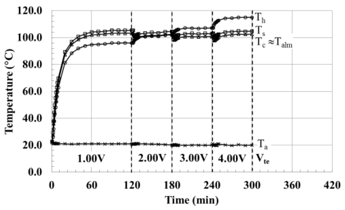
  • Temperature difference between hot and cold sides of the TE (ThTc) is about 36 °C at the low-power input of 10W and about 12 °C at the higher power input of 20W. Temperature difference decreases with TE power input (Pte).
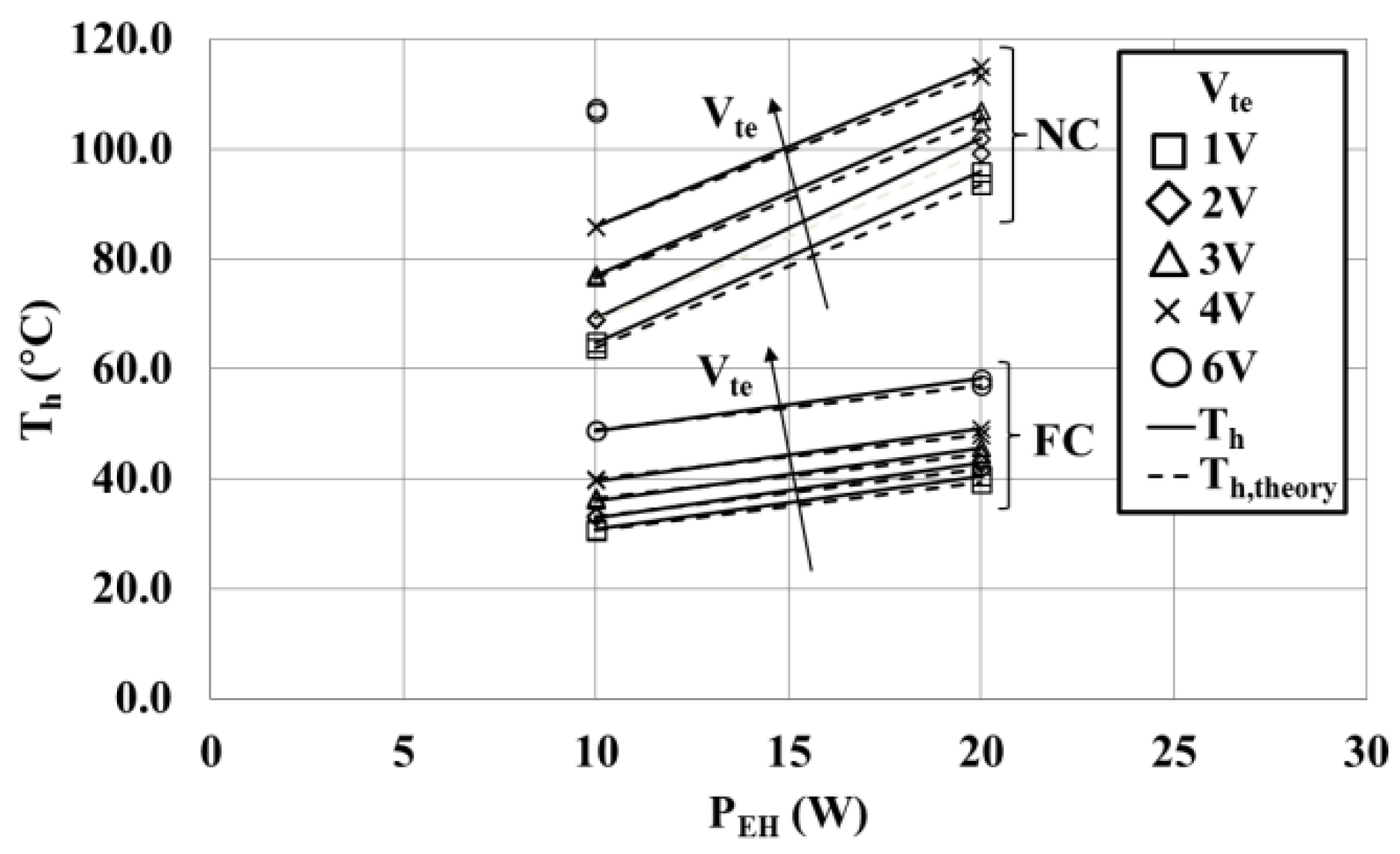
  • Heat source temperature (Ts) increases with power input (PEH) from 73 °C at 10 W to 104 °C at 20 W.
Figure 8 and Figure 9 show the transient temperatures recorded for the hot side (Th), cold (Tc) side, and heat source (Ts) under FC power input (PEH) of 10 W and 20 W, respectively. The following results can be seen:
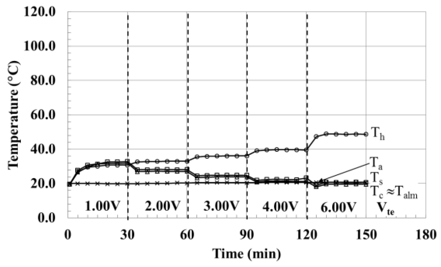
  • Steady-state is achieved earlier under FC compared to NC, i.e., after about 30 min, compared to 120 min and 60 min under NC.
  • Heat source temperature (Ts) is higher than the cold side temperature (Tc) by about 1 °C. A similar difference is observed under NC showing that the contact thermal resistance does not change with convection.
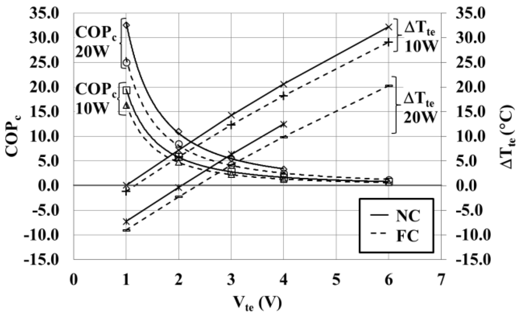
  • Cold side temperature (Tc) decreases with an increase in TE applied voltage (Vte) as expected.
  • The temperature difference (ThTc) between hot and cold sides increase with TE applied voltage (Vte) as expected.
  • Heat source temperature (Ts) wasbrought below, or to, ambient temperature (Ta) when power input (PEH) to the heat source was at 10 W and TE input voltage (Vte) was at 6 V.
  • Heat source temperature (Ts) roseto about 40 °C when the heat source power input (PEH) was increased to 20 W.
  • The temperature difference between TE hot (Th) and cold (Tc) sides was lower at the higher power input of 20 W, comapred to 10 W.
Interface temperatures (Th, Tc, and Ts) under NC and FC conditions and heat source power input (PEH) are compared in Figure 10 and Figure 11. The results show that:
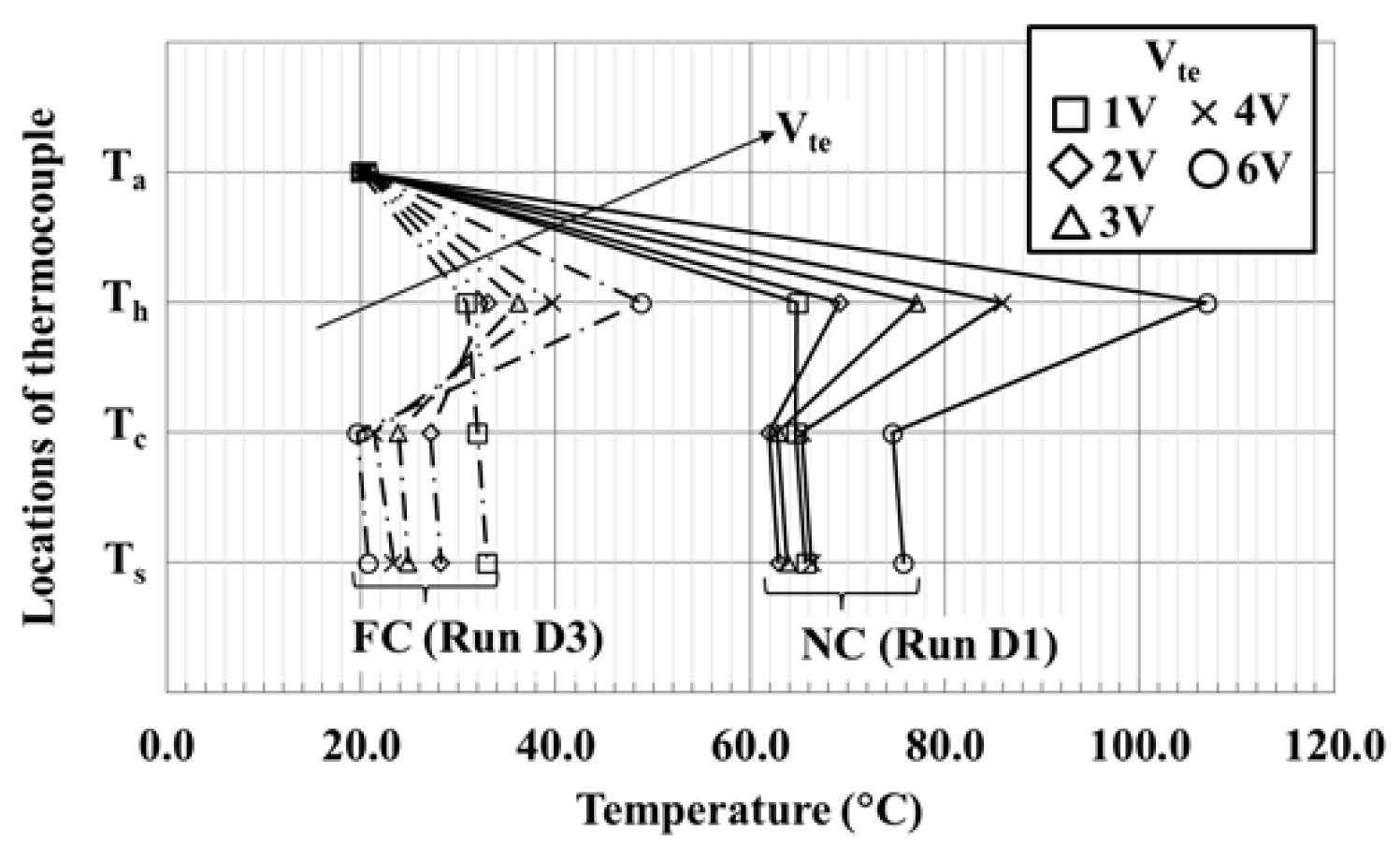
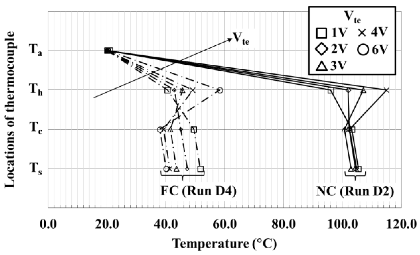
  • All temperatures are lower under FC cooling because of higher cooling heat transfer rates during FC air cooling mode as expected.
  • Hot side (Th) temperatures increase with an increase in the applied TE voltage (Vte).
  • Cold side (Tc) temperatures decrease with an increase in the applied TE voltage (Vte).
  • As a result, the temperature difference between hot and cold sides (ThTc) increase with applied TE voltage (Vte).
  • At low TE applied voltage (Vte), the TE cold side (Tc) could be higher than the hot side (Th). This is because of the insufficient TE power supply to generate a sufficient temperature differential to enable the TE to function.
A comparison between experimental and predicted TE hot side temperature (Th) is shown in Figure 12 at different power inputs (PEH) and under NC and FC modes. It can be seen that the hot side temperature increases with both the heat source and TE power inputs. It is also higher under theNC air flow condition. The predicted values are lower than experimental values by less than 2 °C or about 2%. Keeping in mind that the experimental accuracy of the thermocouples is about +0.5 °C, the agreement between experimental and theoretical is extremely good.
The experimental coefficient of cooling performance (COPc) and temperature difference across the TE module (ΔTte) are compared in Figure 13 at various power inputs to both the heating element (PEH) and the applied voltage (Vte) to the TE and also under NC and FC cooling modes. It can be seen that the temperature difference increases while COPc decreases with TE power input. The NC air flow results in a higher temperature difference and COPc. A higher COPc and lower temperature difference are obtained at higher heat source power input.
The effects of employing a TE module for cooling is shown in Figure 14, which compares the surface temperature of the aluminium block (Talm),with and without the TE module under NC and FC conditions, at 10 W and 20 W power inputs (PEH), and with various applied TE voltage (Vte). The values shown in dashed lines represent the temperature (Talm) obtained without the TE while the solid lines show the results obtained with the FHS-TE assembly. The temperature of the surface of the aluminium block is about 1–2 °C lower than the heating surface temperature (Ts). The results show the following:
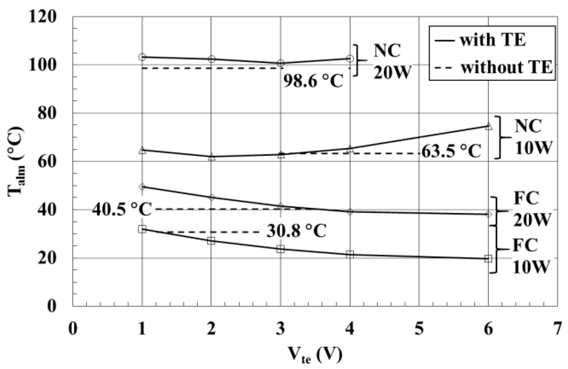
  • The surface temperature of the aluminium block is higher under NC when compared to FC, as expected, because of less efficient cooling.
  • Lower power input (PEH) results in lower temperature.
  • Under the NC cooling mode, the temperature is lower without the use of the TE at both TE applied voltages (Vte) of 10 W and 20 W.
  • In other words, the use of the TE module is not effective under the NC cooling mode. The heat transfer resistance of the TE module has a negative effect on the natural heat loss.
Under the FC cooling at 20 W, the applied voltage (Vte) to the TE module should be >4 V and at 10 W, it should be >1 V.

4. Conclusions

An experimental investigation was conducted to evaluate the thermal cooling performance of a TE module fitted to a conventional FHS and cooled under NC and FC air flows. The results showed that the use of the TE module is not effective under the NC cooling mode. With the present TE module employed, under FC cooling at 20 W, the applied voltage (Vte) to the TE module should be >4 V, and at 10 W, it should be >1 V. A simple iterative method of predicting the hot side temperature of the TE module was presented. Agreement between predicted and experimental values was better than 2%.

Acknowledgments

The study was supported by university internal fund (UTARRF/2015-C1/L01) and Collaborative Research in Engineering, Science and Technology (CREST) under project number P22C2-13.

Author Contributions

K.S.O. and K.C.L. conceived and designed the experiments; C.F.T. and K.C.L. performed the experiments; K.S.O. and C.F.T. analyzed the data; K.C.L. contributed reagents/materials/analysis tools; K.S.O. wrote the paper.

Conflicts of Interest

The authors declare no conflict of interest.

References

  1. Lee, S.; Song, S.; Au, V.; Moran, K.P. Constriction/spreading resistance model for electeronic packaging. In Proceedings of the ASME/JSME Engineering Conference, New York, NY, USA, 19–24 March 1995.
  2. Simons, R.E. Simple formulas for estimating thermal spreading resistance. Electron. Cool. Mag. 2004, 10, 2. [Google Scholar]
  3. Hasan, A.; Hejase, H.; Abdelbaqi, S.; Assi, A.; Hamdan, M.O. Comparative effectiveness of different phase change materials to improve cooling performance of heat sinks for electronic devices. Appl. Sci. 2016, 6. [Google Scholar] [CrossRef]
  4. Ellison, G.N. Maximum thermal spreading resistance for rectangular sources and plates with nonunity aspect ratios. IEEE Trans. Compon. Packag. Technol. 2003, 26, 439–454. [Google Scholar] [CrossRef]
  5. Muzychka, Y.S.; Culham, J.R.; Yovanovich, M.M. Thermal spreading resistance of eccentric heat sources on rectangular flux channels. Trans. ASME 2003, 125, 178–185. [Google Scholar] [CrossRef]
  6. Rowe, D.M. General Principles and basic considerations. In Thermoelectrics Handbook–Macro to Nano; Taylor & Francis: Boca Raton, FL, USA, 2006. [Google Scholar]
  7. Riffat, S.B.; Ma, X. Improving the coefficient of performance of thermoelectric cooling systems: A review. Int. J. Energy Res. 2004, 28, 753–768. [Google Scholar] [CrossRef]
  8. Lee, H.S. Thermal Design Heat Sinks, Thermoelectrics, Heat Pipes, Compact Heat Exchangers, and Solar Cells; Wiley: Hoboken, NJ, USA, 2010. [Google Scholar]
  9. Sasaki, K.; Shindoh, T.; Itoh, Y. Enhancement of energy use efficiency by simultaneous of cooling and heating action during thermoelectric conversion. In Proceedings of the 22nd International Conference on Thermoelectrics, La Grande Motte, France, 17–21 August 2003; pp. 637–640.
  10. Uemura, K.I. Commercial Peltier Modules. In Handbook of Thermoelectrics; Rowe, D.M., Ed.; CRC Press: Boca Raton, FL, USA, 1995. [Google Scholar]
  11. Webb, R.L.; Gilley, M.D.; Zarnescu, V. Advanced heat exchange technology for thermoelectric cooling devices. Trans. ASME 1998, 120, 98–105. [Google Scholar] [CrossRef]
  12. Riffat, S.B.; Ma, X. Optimum selection (design) of thermoelectric modules for large capacity heat pump applications. Int. J. Energy Res. 2008, 28, 1231–1242. [Google Scholar] [CrossRef]
  13. Chein, R.; Huang, G. Thermoelectric cooler application in electronic cooling. Appl. Therm. Eng. 2004, 24, 2207–2217. [Google Scholar] [CrossRef]
  14. Kim, W.T.; Kim, K.S.; Lee, Y. Design of a two-phase loop thermosyphon for telecommunications system. KSME Int. J. 1998, 12, 942–955. [Google Scholar] [CrossRef]
  15. Huang, B.J.; Chin, C.J.; Duang, C.L. A design method of thermoelectric cooler. Int. J. Refrig. 2008, 23, 208–218. [Google Scholar] [CrossRef]
  16. Palacios, R.; Arenas, A.; Pecharroman, R.R.; Pagola, F.L. Analytical procedure to obtain internal parameters from performance curves of commercial thermoelectric modules. Appl. Therm. Eng. 2009, 29, 3501–3505. [Google Scholar] [CrossRef]
  17. Vian, J.G.; Astrain, D. Development of a heat exchanger for the cold side of a thermoelectric module. Appl. Therm. Eng. 2008, 28, 1514–1521. [Google Scholar] [CrossRef]
Figure 1. Thermal cooling with an air-cooled FHS (fin heat sinks) and water-cooled plate heat sink. (a) Air-cooled FHS; (b) Water-cooled plate heat sink.
Applsci 07 00062 g001
Figure 2. Thermal cooling with an air-cooled FHS and TE (thermoelectric).
Applsci 07 00062 g002
Figure 3. Thermal resistance model of the FHS-TE assembly.
Applsci 07 00062 g003
Figure 4. Flowchart to simulate the TE hot side (Th) temperature.
Applsci 07 00062 g004
Figure 5. Experimental apparatus (a); and layout (b) to determine the thermal performance of the FHS-TE assembly.
Applsci 07 00062 g005
Figure 6. Transient temperatures for the FHS-TE assembly (NC (Natural convection), PEH = 10 W, Run D1).
Applsci 07 00062 g006
Figure 7. Transient temperatures for the FHS-TE assembly (NC, PEH = 20 W, Run D2).
Applsci 07 00062 g007
Figure 8. Transient temperatures for the FHS-TE assembly (FC (forced convection), PEH = 10 W, Run D3).
Applsci 07 00062 g008
Figure 9. Transient temperatures for the FHS-TE assembly (FC, PEH = 20 W, Run D4).
Applsci 07 00062 g009
Figure 10. Comparison of interface temperatures for the FHS-TE assembly (NC and FC, PEH = 10 W, Runs D1 and D3).
Applsci 07 00062 g010
Figure 11. Comparison of interface temperatures for the FHS-TE assembly (NC and FC, PEH = 20 W, Runs D2 and D4).
Applsci 07 00062 g011
Figure 12. Comparison of experimental and predicted Th for the FHS-TE assembly.
Applsci 07 00062 g012
Figure 13. Coefficient of performance COPc and temperature difference ΔTte for the FHS-TE assembly.
Applsci 07 00062 g013
Figure 14. Comparison of surface temperature of aluminum block with and without TE.
Applsci 07 00062 g014
Table 1. Experimental results for FHS-TE (fin heat sinks-thermoelectric) assembly under natural (NC) and forced convection (FC).
NC/FCRun #PEH (W)Vte (V)Ite (A)Pte (W)Ta (°C)Ts (°C)TcTalm (°C)Th (°C)ΔTte (°C)Tm (°C)COPcTh,theory (°C)
NCD110.11.010.520.5220.665.764.764.80.164.819.3463.8
10.02.000.851.6920.362.961.969.27.265.55.8968.8
10.03.001.163.5020.363.862.877.114.369.92.8676.6
10.04.011.475.8820.266.365.385.920.675.61.7085.9
10.06.002.0212.1320.075.774.6106.932.390.70.82107.5
D219.91.000.610.6120.9105.4103.296.0−7.299.632.5793.6
19.82.000.901.8120.1104.5102.3102.0−0.4102.110.9799.3
19.83.001.193.5720.2102.9100.7107.16.4103.95.55105.1
19.84.001.475.8820.1104.8102.5115.012.5108.83.37113.3
-6.00----------
FCD310.31.000.630.6319.932.931.930.8−1.131.416.3630.6
10.02.001.042.0820.328.227.133.05.930.04.8033.2
9.93.001.454.3620.524.823.836.112.330.02.2836.5
10.04.001.847.3720.723.321.339.618.330.41.3640.0
10.06.002.6215.720.720.719.648.829.234.20.6348.9
D420.11.000.800.8020.151.749.540.5−9.045.025.0039.3
20.32.011.192.3820.147.345.142.9−2.244.08.5041.7
20.03.001.574.7220.143.641.545.74.243.64.2544.5
20.04.001.967.8419.941.339.249.19.944.22.5548.0
20.36.002.7016.220.340.138.058.320.348.21.2557.0

